Solving Vehicle Routing Problem using Ant Colony Optimisation (ACO) Algorithm

ISSN: 2348-7860 (O) | 2348-7852 (P) | Vol. 5 No. 9 | September-October 2018 | PP.

500-507

Digital Object Identifier DOI

®

http://dx.doi.org/10.21276/ijre.2018.5.9.2

Copyright © 2018 by authors and International Journal of Research and Engineering

This work is licensed under the Creative Commons Attribution International License (CC BY).

creativecommons.org/licenses/by/4.0

|

|

ORIGINAL ARTICLE

Solving Vehicle Routing Problem using

Ant Colony Optimisation (ACO) Algorithm

Author(s):

*Wan Amir Fuad Wajdi Othman,

Aeizaal Azman Abd Wahab

Syed Sahal Nazli Alhady,

Haw Ngie Wong

Affiliation(s):

School of Electrical & Electronic Engineering,

Universiti Sains Malaysia, Malaysia

*

Corresponding Author: [email protected]

Abstract - Engineering field usually requires

having

the

best

design

for

an

optimum

performance, thus optimization plays an important

part in this field. The vehicle routing problem

(VRP) has been an important problem in the field

of distribution and logistics since at least the early

1960s. Hence, this study was about the application

of ant colony optimization (ACO) algorithm to

solve vehicle routing problem (VRP). Firstly, this

study constructed the model of the problem to be

solved through this research. The study was then

focused on the Ant Colony Optimization (ACO).

The objective function of the algorithm was studied

and applied to VRP. The effectiveness of the

algorithm was increased with the minimization of

stopping criteria. The control parameters were

studied to find the best value for each control

parameter. After the control parameters were

identified, the evaluation of the performance of

ACO on VRP was made. The good performance of

the algorithm reflected on the importance of its

parameters, which were number of ants (nAnt),

alpha (α), beta (β) and rho (ρ). Alpha represents the

relative importance of trail, beta represents the

importance of visibility and rho represents the

parameter governing pheromone decay. The route

results of different iterations were compared and

analyzed the performance of the algorithm. The

best set of control parameters obtained is with 20

ants, α = 1, β = 1 and ρ = 0.05. The average cost and

standard deviation from the 20 runtimes with best

set of control parameters were also evaluated, with

1057.839 km and 25.913 km respectively. Last but

not least, a conclusion is made to summarize the

achievement of the study.

Keywords

:

Vehicle Routing Problem, Ant Colony

Optimization, ACO, VRP, Swarm Algorithm

I.

INTRODUCTION

The study is about solving vehicle routing problem (VRP) using ant colony optimization (ACO) algorithm. This is a software-based project. VRP generalizes the well-known travelling salesman problem (TSP). The study can be divided into two parts, vehicle routing problem (VRP) and ant colony optimization (ACO) algorithm.

The vehicle routing problem (VRP) has been an important problem in the field of distribution and logistics since at least the early 1960s [1]. VRP research accelerated during the 1990s [2]. Researchers could develop and implement more complex search algorithms due to the improvement of microcomputer capability and availability. During this era the term meta-heuristics was introduced to name a number of search algorithms for solving these VRPs as well as other combinatorial optimization problems [3].

The technical definition of vehicle routing problem (VRP) states that m vehicles initially located at a depot are to deliver discrete quantities of goods to n customers. The aim of a VRP is to determine the optimal route used by a group of vehicles when serving a group of users. The objective of VRP is to minimize the overall transportation cost. The solution of the classical VRP is a set of routes which all begin and end in the depot, and which satisfies the constraint that all the customers are served only once. The transportation cost can be improved by reducing the total travelled distance and by reducing the number of the required vehicles.

Two important classes of population-based optimization algorithms are evolutionary algorithms and swarm intelligence-based algorithms [3]. In this research, swarm intelligence-based algorithm is chosen to be applied on VRP.

Swarm intelligence-based algorithms is obtained by studying collective intelligence which exist in nature such a cockroach, fish, ant, bee, birds and so on. The pattern of their survival can be presented with algorithm.

When the task is about the optimization within complex domains of data or information, the solutions are methods representing successful animal and micro-organism team behavior, such as swarm or flocking intelligence (birds flocks or fish schools inspired Particle Swarm Optimization), artificial immune systems (that mimic the biological one), ant colonies (ants foraging behaviors gave rise to Ant Colony Optimization), or optimized performance of bees, etc. [3].

The study is focused on the general vehicle routing problem (VRP). There are many other methods regarding VRP as discussed earlier in this section while this project is focusing on ant colony optimization (ACO) algorithm.

II. RELATED

WORKS

A. Vehicle Routing Problem

Vehicle routing problems (VRPs) are an extension of the classic travelling salesman problem (TSP). In this problem, one or more vehicles travel around a network, leaving from and returning to a depot node. The customers are located on the network and each customer must be visited by exactly one vehicle once. Customers are usually located at network nodes.

The objective of the VRP is to find the vehicle routing(s) of minimum cost or in other word, to minimize the total route length [3]. It is described as finding the minimum distance or cost of the combined routes of a number of vehicles m that must service a number of customer n [4].

Mathematically, the system of the VRP is described as a weighted graph G = (V, A, d) where the vertices are represented by V= {v0, v1 ... vn} and the arcs are represented by A= {(vi, vj) : i≠j}. A central depot where each vehicle begins its route is located at v0 and each of the other vehicles represents the n customers [4]. The distance connected with each arc are represented by the variable dij, which are associated with each arc (vi, vj), represent the distance (or the travel time or the travel cost) between vi and vj [5].

The VRP is solved under a few constraints as follows: 1. Each customer is visited only once by a single vehicle. 2. Each vehicle must start and end its route at the depot, v0. 3. For each vehicle route, total route length does not exceed maximum route length, Lm, which includes a service distance δ for each customer on the route.

4. VRP studied here is symmetrical where dij= dji for all i and j.

B. Ant Colony Optimization (ACO) Algorithm

Ant colony optimization (ACO) metaheuristic, a novel population-based approach was proposed by Dorigo et al. to solve several discrete optimization problems [6]. ACO is one of the techniques for approximate optimization. The inspiring source of ACO algorithms are real ant colonies. ACO algorithm mimics the way real ants find the shortest route between the food source and their nest. The ants’ foraging behavior is the main idea of the algorithms. The indirect communication between the ants is the core of this behavior.

The communication between ants is done by depositing a chemical substance called pheromone. As an ant travels, it deposits a constant amount of pheromone that other ants can follow. However, the continuous random selection of paths by individual ants helps the colony to discover alternate routes when they meet a new decision point. The ants can choose to follow the pheromone trail which will reinforce the path and increase the probability of the next ant following the trail, or they can select a new path. Pheromone trails enables them to find short paths between their nests and food sources.

The path with higher concentration of pheromone is more likely to be chosen and thus reinforced. More and more ants are soon attracted to the path and hence the optimal route from the nest to food source and back is very quickly established. In the meantime, the pheromone intensity of the other paths that are not chosen is decreased through evaporation. The unchosen paths become difficult to detect and thus further decreases their use. This phenomenon is called stigmergy, which is defined as a mechanism of indirect coordination, through the environment, between agents or action.

The principle of stigmergy is that the trace left in the environment by an action stimulates the performance of a next action, by the same or a different agent [7]. This characteristic of real ant colonies is exploited in ACO algorithms in order to solve VRP.

Fig. 1 shows how real ants find the shortest path. In Figure 1(A), the ants arrive at a decision point. In Figure 1(B), some ants choose the upper path and some the lower path (the choice is random). In Figure 1(C), given the ants move at approximately a constant speed, the ants that choose the lower path which is shorter reach the opposite decision point faster than those which chose the upper path which is longer. The ants then go back to the starting point using the same path and thus reinforce the pheromone of the route. In Figure 1(D), pheromone accumulates at a higher rate on the shorter path which is represented by number of dashed lines in the figure.

Fig. 1. Real Ant Action [8]

III.

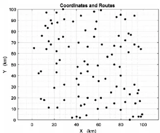
METHODOLOGY

The section discusses the implementation of Ant Colony Optimization (ACO) algorithm to solve vehicle routing problem (VRP). Fig. 2 shows the overall flow chart for the methodology of this work.

A. Ant Colony Optimization (ACO) Algorithm

ACO are divided into two main phases, which are ants’ route construction and the pheromone update [3]. In the first phase, which is tour construction phase, M ants concurrently chosen in the network of N customer nodes (plus the depot node)? At each construction step, ant k currently at node i applies a probabilistic random proportional rule to decide which node to go to next. It selects the move to expend its tour by taking into account the following two values, heuristic function ηij and the level of pheromone on the arc

(i, j), denoted τij. The ηij represents the attractiveness of the

move, usually calculated as the inverse of the distance/cost on the arc from the node i to node j. The τij indicates how

useful it has been in the past to traverse this particular arc. Probabilistic random proportional rule are shown below:

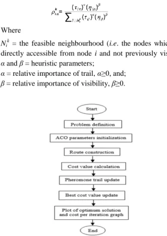
(1) Where

Nik = the feasible neighbourhood (i.e. the nodes which are

directly accessible from node i and not previously visited); α and β = heuristic parameters;

α = relative importance of trail, α≥0, and; β = relative importance of visibility, β≥0.

Equation (1) is the probabilistic random proportional rule that calculate the probability that the ant k chooses to go to node n next.

For first phase, which is during route construction, ant k located at node i moves to node n chosen according to the

Eq. (1). Then, after ant k moves to the next node, the new

node become the node i while another new node n is chosen again according to the probabilistic random proportional rule.

This phase is repeated with the condition that the same node cannot be chosen twice, which means that every node will only undergo this phase once. For second phase, pheromone updates of ACO are very critical to achieve optimum solution. The pheromone updating formula was meant to stimulate the change in the amount of pheromone due to both the accumulation of new pheromone deposited by ants on the visited edges and the pheromone evaporation [8]. ACO algorithm uses two types of pheromone updates, namely global pheromone update and local pheromone update.

The local pheromone update is performed every time an ant transverses an arc (i, j) by using Eq. 2 below;

(2) Where:

τ0= 1/(NLnn),

τ0 = the initial pheromone value, and

Lnn = the length of the nearest neighbor tour (a tour in

which each move is to the nearest unvisited node; this is used as a baseline tour length).

The global pheromone update is only carried out by the ant that produced the best tour so far and is implemented by Eq. 3 for each arc of the tour.





 

ij

ρ

τ

+

ρΔτ

,

i,

j

T

τ



1







Where

Δτijbs = Q/Lbs

ρ = parameter governing pheromone decay, Q = constant, and

Tbs = the best found tour so far with Lbs as its length.

B. Control Parameters of ACO Algorithm

Since the optimization problem involved in this study consists of four different control parameters that can affect the output of the algorithm, the algorithm will be evaluated according to the different combinations of these parameters.

Table 1 shows the setting for these control parameters that are used to evaluate the performance and output of the algorithm.

C. Comparative Study on Cost Function and Stopping Criteria

The objective function was Equation 1. To decide the stopping criteria, the algorithm was executed at maximum of 500 iterations at first. Then, to determine the termination condition, one-third or two-third of the iterations executed were taken as the maximum iterations for the algorithm or in other words, when a steady cost value was obtained. After the suitable stopping criteria were selected, several sets of control parameters were selected. The algorithm was executed with the selected set of control parameters. The data output of the algorithm was extracted and compared. The number of runtimes was one of the stopping criteria in this algorithm. The algorithms were executed with 20 runtimes for each set of control parameters. Each runtime was an independent experiment which did not affect the other experiments.

Results obtained from the 20 runtimes were tabulated and compared to check the robustness of the algorithm. The comparison and analysis of the different sets of control parameters can lead to the best set of control parameters among all.

The average cost value was calculated by summing up the values of cost values from runtime 1 to runtime 20 and divided by the total number of runtimes which was 20 runtimes. The average cost values were tabulated. Theoretically, the cost values were significantly reduced through iterations and finally converged to a final best value.

As the algorithm found the final best value, the cost value was the optimal solution and will be constant throughout the rest of the iterations. The solutions can be said to be improving in the next iteration. To visualise the convergence of cost values, the graph of average cost function against number of iterations was plotted. Besides, error bars were plotted in both graphs to indicate the variability of data. The plots were compared for ACO algorithms with different set of control parameters. The results of the algorithm were compared in terms of computational time, cost function values and converges. The combination of different control parameters were tested to find the best combination of the control parameters.

IV.

R

A. Construction of VRP

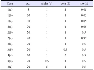
In ant colony optimization (ACO) algorithm, the VRP was represented by using a graph while the customers were represented by using the nodes on the graph. The range of graph was set to be from 0 to 100 for both x-axis and y axis. In order to evaluate the performance of the algorithm, the fixed coordinates were used in the algorithm. The number of the nodes (aka the customers) was set to 100. Fig. 3 shows the fixed coordinates that were used for the rest of the study.

B. Selection of Stopping Criteria

The stopping criteria of the algorithm were the number of iteration. In order to determine the suitable number of iteration, the algorithm was first executed with 500 iterations. The parameters used for the evaluation are 20 ants, alpha, α = 1, beta, β =1, rho, ρ = 1 & 0.05. The optimum result obtained and reviewed to determine the termination condition.

Fig. 4 shows the result for 500 iterations. The graph indicated that the algorithm achieved the optimum result around 100-150 iterations. Thus, the stopping criteria of the algorithm for the rest of the thesis was set to be 150 iterations as it was good enough to obtain the optimum result required without wasting too much execution time and accumulate too much excessive data to be reviewed.

Fig. 3 Coordinates of customers TABLE I. SETTING OF PARAMETERS

Parameters Settings

nAnt 5, 20, 30

alpha (α) 0.5, 1, 5

beta (β) 0.5, 1, 5

C. Selection of Best Set of Control Parameters

The algorithm will be executed with different set of control parameters. Table 2 shows the control parameters that will be considered. Meanwhile, the stopping criteria (number of iterations) were set to be constant as discussed in previous session.

1) Parameter 1: Number of Ant (nAnt)

The ants in the ant colony algorithm (ACO) algorithm represented the vehicles in the vehicle routing problem (VRP). The number of vehicle was one of the control

parameters that affect the performance of the algorithm. According to Table 2, the number of ants was set to 5, 20 and 30. The algorithm was executed 30 times each with different number of ants. The performance of the algorithm was the best when the number of ants was set to be 20 (Case 1(b)). The number of iteration required to obtain the optimal result was shortest and was within two-third of the stopping criteria. The result was more accurate as compared to Case 1(a) and Case 1(c).

2) Parameter 2: rho (ρ)

The parameter rho (ρ) was used in most of the formulas in the ACO algorithm. The parameter was limited at range of (0<ρ<1). According to Table 2, rho was set to 0.05, 0.50 and 0.99. The algorithm was executed 30 times each with different value of rho. The performance of the algorithm was the best when the value of rho was set to be 0.05 (Case 2(a)). The average time elapsed for the algorithm was shortest among Case 2. The number of iteration required to obtain the optimal result was in the acceptable range which was around two-third of the stopping criteria. Furthermore, the result was more accurate as compared to the other two value of rho as the range of result obtained was smaller and more precise.

Table 3 shows the comparison of data obtained in Case 2.

The constant best cost value after the optimal result was obtained became the proof that there was no further best cost value. The best cost value for each case was almost the same and thus it did not affect the choice too much.

3) Parameter 3: Alpha (α) and Beta (β)

Alpha (α) and beta (β) were control parameters that affect the performance of the algorithm. According to Table 2, five pairs of alpha and beta were either 0.5, 1 or 5. The algorithm was executed 30 times each with different combination of alpha and beta.

The performance of the algorithm was compared with the tabulated data. From Table 4, the performance of the algorithm was the best when the value of the alpha and beta was set to 1 respectively (Case 3(a)). The average time elapsed for the algorithm was the shortest among Case 3. The average best cost value of Case 3(a) was slightly larger than that in Case 3(c), but there was significant improvement in terms of averaged time elapsed. Case 3(b), case 3(d) and case 3(e) were not suitable for the study because the average best Fig. 4 Result for 500 iterations

TABLEII.SETS OF CONTROL PARAMETERS

Case nAnt alpha (α) beta (β) rho (ρ)

1(a) 5 1 1 0.05 1(b) 20 1 1 0.05 1(c) 30 1 1 0.05 2(a) 20 1 1 0.05 2(b) 20 1 1 0.5 2(c) 20 1 1 0.99 3(a) 20 1 1 0.5 3(b) 20 1 0.5 0.5 3(c) 20 1 5 0.5 3(d) 20 0.5 1 0.5 3(e) 20 5 1 0.5

TABLEIII.DATA OF CASE 2

Max-iteration Min-iteration Range

Case 2(a) 148 65 83

Case 2(b) 146 34 112

Case 2(c) 106 20 86

TABLEIV.DATA OF CASE 3 Case Parameters Average

elapsed time (s) Average best cost value Average iteration 3(a) α=1, β=1 16.700 1054.61 111.7 3(b) α=1, β=0.5 18.951 1404.17 119.75 3(c) α=1, β=5 22.725 892.01 81.25 3(d) α=0.5, β=1 16.759 1823.48 110.35 3(e) α=5, β=1 22.023 1627.08 9.6

cost value was obviously higher when compared to that of case 3(a).

D. Comparative Study on Best Cost Value of ACO

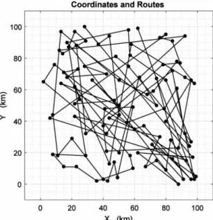
The algorithm was executed 30 times with the parameter settings as follow: nAnt = 20, α=1, β=1, ρ=0.05 and 1 vehicle. The best cost per iteration of each runtime was tabulated for analysis. The result of Runtime 16 was shown for discussion as the elapsed time and best cost value were below average.

Fig. 5 shows the optimum route result while Fig. 6 shows the graph of best cost per iteration. Both of the results were taken from Runtime 16. The optimum route results were never exactly the same with one another as every runtime was independent with others.

In Fig. 6, the best cost values against iteration are plotted in the graph. The minimum cost was informed in the title of the graph. The data implied that the total distance travelled by the vehicle to reach all the customers once was 1043.3716

km.

1) Route Analysis

Five route results were taken from the same runtime to show the progress of the route construction as the number of iteration increases. The graphs were taken from Runtime 1. The route results were taken at first iteration (Fig. 7) and then when the optimal results were reached (Fig. 8). The algorithm was proven to obtain new best cost value and minimum route in increasing iteration until the optimal result is achieved.

2) Cost Value Analysis

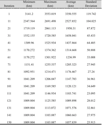
The average cost value and standard deviation for each iteration was calculated and tabulated. The data was used to plot the graph of average cost versus iteration.

Table 5 tabulates the minimum, maximum average and

standard deviation of the cost; whilst error bars plot in Fig.9

shows the standard deviation per iterations. The standard deviation shows how spreads out the cost values are and reflects the confidence of cost value evaluated by the algorithm. Considering the graph, it can be seen that the standard deviation decreased significantly from the previous iterations.

V. CONCLUSION

In conclusion, the objectives of this study have been achieved. This study aims to solve vehicle routing problem using swarm algorithm. The swarm algorithm used in this study was ant colony optimization (ACO) algorithm. To achieve this aim, stopping criteria and four control parameters were outlined in the earlier stage of research to present the best possible algorithm for the vehicle routing problem. It can be deducted that the application of ACO for VRP are successfully conducted. The overall performance of the algorithm is as good as expected. Further study can be Fig. 5 Optimal route found on runtime 16

FIG. 6. Cost against iteration for Runtime 16

TABLE V,AVERAGE COST AGAINST ITERATION FOR 20 SIMULATION-RUN Iteration Minimum (km) Maximum (km) Average (km) Standard Deviation 1 3141.2 3553.019 3350.555 119.742 11 2347.564 2691.498 2527.852 104.025 21 1719.119 2061.113 1950.31 87.872 31 1552.155 1720.585 1658.041 45.433 41 1309.96 1525.934 1437.864 64.485 51 1170.272 1374.362 1314.668 50.888 61 1170.272 1301.922 1236.99 33.008 71 1151.41 1255.537 1205.323 27.945 81 1092.951 1214.471 1176.467 27.24 91 1041.209 1206.047 1147.783 36.961 101 1041.209 1169.585 1120.121 34.649 111 1041.209 1146.934 1103.741 23.095 121 1009.804 1125.585 1089.898 28.012 131 1009.804 1113.072 1071.576 32.861 141 1009.804 1103.887 1060.663 27.975 150 1009.804 1103.887 1057.839 25.913

made to apply different swarm algorithm to VRP. The advantages of ACO algorithm should be exploited to solve different optimization problems. The study of ACO optimization can also be synchronized with the internet to be used in real life.

VI.

DECLARATION

All authors have disclosed no conflicts of interest, and authors would like to thank the Ministry of Education Malaysia and Universiti Sains Malaysia for supported the work by Fundamental Research Grant Scheme (Grant number: USM/PELECT/6071239).

REFERENCES

[1] G. B. Dantzig and J. H. Ramser, "The Truck Dispatching Problem", Management Science, vol. 6, pp. 80-91, 1//1959.

[2] G. Laporte, "Fifty Years of Vehicle Routing", Transportation Science, vol. 43, pp. 408-416, 4// 2009.

[3] M. Reed, A. Yiannakou, and R. Evering, "An ant colony algorithm for the multi-compartment vehicle routing problem," Applied Soft Computing, vol. 15, pp. 169-176, 2// 2014.

[4] J. E. Bell and P. R. McMullen, "Ant colony optimization techniques for the vehicle routing problem," Advanced Engineering Informatics, vol. 18, pp. 41-48, 1// 2004.

[5] B. Bullnheimer, R. F. Hartl, and C. Strauss, "An improved Ant System algorithm for theVehicle Routing Problem," Annals of Operations Research, vol. 89, pp. 319-328, 1999.

[6] Z. Song, G. Ming, L. Chunfu, W. Chunlin, and X. Anke, "New transition probablity for Ant Colony Optimization: global random-proportional rule," in 2010 8th World Congress on Intelligent Control and Automation, 2010, pp. 2698-2702.

FIG. 8. Best route result for iteration = 80 in runtime 1

[7] G. Theraulaz and E. Bonabeau, "A Brief History of Stigmergy," Artificial Life, vol. 5, pp. 97-116, 1999. [8] M. Dorigo and L. M. Gambardella, "Ant colony

system: a cooperative learning approach to the traveling salesman problem," IEEE