A Self-Learning Particle Swarm Optimizer for
Global Optimization Problems
Changhe Li, Shengxiang Yang
Member, IEEE
, and Trung Thanh Nguyen
Abstract—Particle swarm optimization (PSO) has been shown as an effective tool for solving global optimization problems. So far, most PSO algorithms use a single learning pattern for all particles, which means all particles in a swarm use the same strategy. This monotonic learning pattern may cause the lack of intelligence for a particular particle, which makes it unable to deal with different complex situations. This paper presents a novel algorithm, called self-learning particle swarm optimizer (SLPSO), for global optimization problems. In SLPSO, each particle has a set of four strategies to cope with different situations in the search space. The cooperation of the four strategies is implemented by an adaptive learning framework at the individual level, which can enable a particle to choose the optimal strategy according to its own local fitness landscape. The experimental study on a set of 45 test functions and two real-world problems show that SLPSO has a superior performance in comparison with several other peer algorithms.
Index Terms—Self-learning particle swarm optimization (SLPSO), particle swarm optimization (PSO), operator adapta-tion, topology adaptaadapta-tion, global optimization problem.
I. INTRODUCTION
E
VOLUTIONARY computation has become an important active research area over the past several decades. In the literature, global optimization benchmark problems have become more and more complex, from simple unimodal functions to rotated shifted multi-modal functions to hybrid composition benchmark functions proposed recently [41]. Finding the global optima of a function has become much more challenging or even practically impossible for many problems. Hence, far more effective optimization algorithms are always needed.In the past decade, PSO has been actively studied and applied for many academic and real-world problems with promising results [33]. However, many experiments have shown that the basic PSO algorithm easily falls into local optima when solving complex multi-modal problems [25] with a huge number of local optima. In the literature of PSO, for most algorithms so far, all particles in a swarm use only a single learning pattern. This may cause the lack of intelligence for a particle to cope with different complex situations. For
Manuscript received June 01, 2011; accepted September 23, 2011. This work was supported by the Engineering and Physical Sciences Research Coun-cil (EPSRC) of U. K. under Grant EP/E060722/1 and Grant EP/E060722/2.
C. Li is with the School of Computer Science, China University of Geosciences, Wuhan, 430074, China (email: [email protected]).
S. Yang is with the Department of Information Systems and Computing, Brunel University, Uxbridge, Middlesex, UB8 3PH, U. K. (email: [email protected]).
T. T. Nguyen is with The School of Engineering, Technology and Mar-itime Operations, Liverpool John Moores University, Liverpool L3 3AF, U. K. (email: [email protected]).
example, different problems may have different properties due to different shapes of the fitness landscapes. In order to effectively solve these problems, particles may need different learning strategies to deal with different situations. This may also be true even for a specific problem because the shape of a local fitness landscape in different sub-regions of a specific problem may be quite different, such as the composition benchmarks in [41].
To bring more intelligence to each particle, an adaptive learning PSO algorithm (ALPSO) that utilizes four strategies was introduced in [21], where each particle has four learning sources to serve the purpose of exploration or exploitation during the search process. An adaptive technique proposed in [22] was used to adjust a particle’s search behavior between exploration and exploitation by choosing the optimal strategy. Based on our previous work in [21], a novel algorithm, called self-learning PSO (SLPSO), is proposed in this paper. Compared with ALPSO, some new features are introduced in SLPSO. Firstly, two strategies in ALPSO are replaced by two new strategies. Secondly, we use a biased selection method in SLPSO so that a particle learns from only the particles whosepbests are better than itspbest. Thirdly, the method of updating the frequency parameter in ALPSO is replaced by a new one. Fourthly, we introduce a super particle generated by extracting promising information from improved particles instead of directly updating the gbest particle, where the extracting method is also enhanced by using a learning ratio. Fifthly, controlling the number of particles that learn from the super particle is implemented. Finally, although some new parameters are introduced in SLPSO, users do not need to tune these parameters for a specific problem as they use the same setting up methods for all problems.
The rest of this paper is organized as follows. Section II describes the basic PSO algorithm and some variants. The SLPSO algorithm is presented in Section III. Section IV describes the test problems and experimental setup. The experimental study on SLPSO, including the self-learning mechanism and sensitivity analysis of parameters, is presented in Section V . The performance comparison of SLPSO with some peer algorithms taken from the literature is given in Section VI. Finally, Section VII concludes this paper.
II. RELATEDWORK A. Particle Swarm Optimization
Similar to other evolutionary algorithms (EAs), PSO is a population based stochastic optimization technique. A poten-tial solution in the fitness landscape is called a particle in PSO.
Each particle i is represented by a position vector ~xi and a
velocity vector~vi, which are updated as follows:
v0di =ωvid+η1r1(xdpbesti−x
d
i) +η2r2(xdgbest−xdi) (1)
x0di =xdi +v0di, (2) wherex0d
i andxdi represent the current and previous positions
in the d-th dimension of particlei, respectively,v0
i andvi are
the current and previous velocity of particle i, respectively, ~
xpbesti and~xgbest are the best position found by particleiso
far and the best position found by the whole swarm so far, respectively,ω∈(0,1)is an inertia weight, which determines how much the previous velocity is preserved; η1 and η2 are
the acceleration constants, andr1andr2are random numbers
generated in the interval[0.0,1.0]uniformly. Without loss of generality, minimization problems are considered in this paper. There are two main models of the PSO algorithm, called gbest(global best) andlbest(local best), respectively. The two models differ in the way of defining the neighborhood for each particle. In the gbest model, the neighborhood of a particle consists of the particles in the whole swarm, which share information between each other. On the contrary, in the lbest model, the neighborhood of a particle is defined by several fixed particles. The two models give different performances on different problems. Kennedy and Eberhart [19] and Poli
et al. [33] pointed out that the gbest model has a faster convergence speed but also has a higher probability of getting stuck in local optima than the lbestmodel. On the contrary, the lbest model is less vulnerable to the attraction of local optima, but has a slower convergence speed than the gbest model. In order to give a standard form for PSO, Bratton and Kennedy proposed a standard version of PSO (SPSO)1in [5]. In SPSO, a local ring population topology is used and the experimental results have shown that the lbestmodel is more reliable than the gbest model on many test problems.
B. Some Variant Particle Swarm Optimizers
Due to its simplicity and effectiveness, PSO has become a popular optimizer and many improved versions have been reported in the literature since it was first introduced. Most studies address the performance improvement of PSO from one of four aspects: population topology [25], [18], [20], [24], [29], [40], diversity maintenance [3], [4], [6], [21], [34], hybridization with auxiliary operations [1], [32], [46], and adaptive PSO [15], [34], [36], [37], [52], which are briefly reviewed below.
1) Population Topology: The population topology has a significant effect on the performance of PSO. It determines the way particles communicate or share information with each other. Population topologies can be divided into static and dynamic topologies. For static topologies, communication structures of circles, wheels, stars, and randomly-assigned edges were tested in [18], showing that the performance of algorithms is different on different problems depending on the
1Notice that the term “SPSO” in this paper indicates the standard version of PSO in [5] rather than the speciation-based PSO in [23], which will be introduced later.
topology used. Then, Kennedy and Mendes [20] have tested a large number of aspects of the social-network topology on five test functions. After that, a fully informed PSO (FIPS) algorithm was introduced by Mendes [29]. In FIPS, a particle uses a stochastic average of pbests from all of its neighbors instead of using its ownpbestposition and thegbestposition in the update equation. A recent study in [24] showed that PSO algorithms with a ring topology are able to locate multiple global or local optima if a large enough population size is used.
For dynamic topologies, Suganthan [40] suggested a dynam-ically adjusted neighbour model, where the search begins with albestmodel and is gradually increased until thegbestmodel is reached. Janson et al. proposed a dynamic hierarchical PSO (H-PSO) [16] to define the neighborhood structure where particles move up or down the hierarchy depending on the quality of their pbest solutions. Liang and Suganthan [25] developed a comprehensive learning PSO (CLPSO) for multi-modal problems. In CLPSO, a particle uses different particles’ historical best information to update its velocity, and for each dimension a particle can potentially learn from a different exemplar.
2) PSO with Diversity Control: Ratnaweera et al. [34] stated that the lack of population diversity in PSO algorithms is a factor that makes them prematurely converge to local optima. Several approaches of diversity control have been introduced in order to avoid the whole swarm converging to a single opti-mum. In [3], diversity control was implemented by preventing too many particles from getting crowded in one region of the search space. Negative entropy was added into PSO in [49] to discourage premature convergence. Other researchers have applied multi-swarm methods to maintain diversity in PSO. In [6], a niching PSO (NichePSO) was proposed by incorporating a cognitive only PSO model with the guaranteed convergence PSO (GCPSO) algorithm [45]. Parrott and Li developed a speciation based PSO [23], which dynamically adjusts the number and size of swarms by constructing an ordered list of particles, ranked according to their fitness, with spatially close particles joining a particular species. An atomic swarm approach was adapted to track multiple optima simultaneously with multiple swarms in dynamic environments by Blackwell and Branke [4]. Recently, a clustering PSO algorithm was proposed in [50], where a hierarchical clustering method is used to produce multi-swarms in promising regions in the search space.
3) Hybrid PSO: Hybrid EAs are becoming more and more popular due to their capabilities in handling problems that involve complexity, noisy environments, imprecision, uncer-tainty, and vagueness. Among hybrid EAs, hybrid PSO is an attractive topic. The first hybrid PSO algorithm was developed by Angeline [1], where a selection scheme is introduced. In [46], the fast evolutionary programming (FEP) [51] was modified by replacing the Cauchy mutation with a version of PSO velocity. Hybrid PSO based on genetic programming was proposed in [32]. A cooperative PSO (CPSO-H) algorithm was proposed in [44], which employs the idea of splitting the search space into smaller solution vectors and combines with thegbestmodel of PSO. In [7], a hybrid model that integrates
PSO, recombination operator, and dynamic linkage discovery, called PSO-RDL, was proposed.
4) PSO with Adaptation: Besides the above three active research aspects, adaptation is another promising research trend in PSO. Shi and Eberhart introduced a method of linearly deceasing ω with the iteration for PSO in [36], and then proposed a fuzzy adaptive ω method for PSO in [37]. Ratnaweeraet al.[34] developed a self-organizing hierarchical PSO with time-varying acceleration coefficients, whereη1and
η2 are set to a large value and a small value, respectively, at
the beginning, and are gradually reversed during the search process. By considering a time-varying population topology, FIPS’s velocity update mechanism [29], and a decreasing inertia weight, a PSO algorithm, called Frankenstein’s PSO (FPSO), was proposed in [11]. In FPSO, the swarm starts with a fully connected population topology. The connectivity decreases with a certain pattern and ends up with the ring topology. The performance of a TRIBES model of PSO was investigated in [8], which is able to automatically change the behavior of particles as well as the population topology. A population manager method for PSO was proposed in [15], where the population manager can dynamically adjust the number of particles according to some heuristic conditions defined in [15].
Recently, a PSO version with adaptiveω,η1, andη2, called
APSO, was proposed by Zhanet al.[52]. In APSO, four evo-lutionary states, including “exploitation”, “exploration”, “con-vergence”, and “jumping out”, are defined. Co-incidentally, the four operators in ALPSO [21] play the similar roles as the four evolutionary states defined in APSO [52], but the way of implementation is different. While the four operators in ALPSO are updated by an operator adaptation scheme [21], the evolutionary states in APSO are estimated by evaluat-ing the population distribution and particle fitness. In each evolutionary state, APSO gives one corresponding equation to adjust the value of η1 and η2. Accordingly, the value
of ω is tuned using a sigmoid mapping of the evolutionary factorf in each evolutionary state. Similar work of adaptively tuning the parameters of PSO has been done in [48], [31]. However, none or little work of operator selection has been done in PSO. Experimental study in [21] has shown that the adaptive learning approach is an effective method to improve the performance of PSO.
C. Self-learning and Adaptive Strategies
Swarm intelligence (SI) is the property of a system whereby the collective behaviors of (unsophisticated) agents interacting locally with their environment cause coherent functional global patterns to emerge [47]. Agents (individuals) have some simple interaction rules and each agent is able to adjust its behavior according to the results of interaction with local environments. Complex, emergent, and collective behaviors are shown up only based on simple interactions with local environments. However, it is difficult for us to understand and simulate the emergent behaviors from nature to solve real-world problems. Although it is difficult to exactly simulate the emergent collective behaviors, we can employ techniques based on
adaptive operator selection (AOS) to implement the adaptive behavior of social creature groups, e.g., ant colony, bee colony, and bird flocking, etc. AOS is an important step toward self-tuning for EAs. To design an efficient AOS structure, generally, we need to solve two issues: a credit assignment mechanism, which computes a reward for each operator at hand based on certain rules from statistical information of offspring; and an adaptation mechanism, which is able to adaptively select one among different operators based on their rewards [9], [12], [14], [39], [38], [42], [43].
The low-level behavior of the choice-function based hyper-heuristic was investigated in [17]. Based on the fact that no single operator is optimal for all problems and the optimal choice of operators for a given problem is also time-variant, Smith and Fogarty [39] suggested a framework for the classifi-cation based on the learning strategy used to control them and reviewed a number of adaptation methods in GAs. Thereafter, to address the issue that the set of available operators may change over time, Smith [38] proposed a method for estimating an operator’s current utility, which is able to avoid some of the problems of noise inherent in simpler schemes for memetic algorithms. In [42], [43], an adaptive allocation strategy, called the adaptive pursuit method, was proposed and compared with some other probability matching approaches in a controlled, dynamic environment. In [9], a specific dynamic method based on the multi-armed bandit paradigm was developed for dy-namic frameworks. In order to well evaluate the performance of operators, recently, a new strategy [27] was introduced by considering not only the fitness improvements from parent to offspring, but also the way they modify the diversity of the population, and their execution time.
III. SELF-LEARNINGPARTICLESWARMOPTIMIZER A. General Considerations of Performance Tradeoff
It is generally believed that the gbest model biases more toward exploitation, while the lbest model focuses more on exploration. Although there are many improved versions of PSO, the question of how to balance the performance of the gbest andlbestmodels is still an important issue, especially for multi-modal problems.
In order to achieve good performance, a PSO algorithm needs to balance its search between the lbest and gbest models. However, this is not an easy task. If we let each particle simultaneously learn from both itspbestposition and the gbest or lbestposition to update itself (velocity update), the algorithm may suffer from the disadvantages of both models. One solution might be to implement the cognition component and the social component separately. This way, each particle can focus on exploitation by learning from its individualpbestposition or focus on convergence by learning from thegbestparticle. The idea enables particles of different locations in the fitness landscape to carry out local search or global search, or vice versa, in different evolutionary stages. So, different particles can play different roles (exploitation or convergence) during the search progress, and even the same particle can play different roles during different search progress.
Algorithm 1 Update(operatori, particlek,f es)
1:ifi=athen
2: Update the velocity and position of particlekusing operatoraand Eq. (2);
3:else ifi=bthen
4: Update the position of particlekusing operatorb;
5:else ifi=cthen
6: Choose a random particlejthat is not particlek;
7: iff(~xpbestj)< f(~xpbestk)then
8: Update the velocity and position of particlekusing operatorcand Eq. (2);
9: else
10: Update the velocity and position of particlejusing operatorcand Eq. (2);
11: k:=j;
12: end if
13: else
14: Update the velocity and position of particlekusing operatordand Eq. (2);
15: end if
16: f es++; wheref esis the current number of fitness evaluations.
However, there is a difficulty in implementing this idea: the appropriate moment for a particle to learn from gbest or pbest is very hard to know. To implement the above idea, we introduce an adaptive method to automatically choose one search strategy. In this method, which strategy to apply and when to apply that strategy are determined by the property of the local fitness landscape where a particle is located. This adaptive method will be further described in the following sections.
B. Velocity Update in SLPSO
Inspired by the idea of division of labor, we can assign different roles to particles, e.g., converging to the global best particle, exploiting the personal best position, exploring new promising areas, or jumping out of local optima. Accordingly, we summarize four different possible situations regarding surrounding environments for a general particle. Firstly, for unimodal problems or the fitness landscape with peaks that are far away from each other, to effectively search on local peaks, the best learning policy for all particles may be to learn from their neighbour best particles. Secondly, for a particle in a slope, the best strategy may be to learn from its own pbest position as it will help the particle to find a better position much easier than searching in a distant sub-region. Thirdly, for the fitness landscape with many local optima evenly distributed, learning from neighbors may be the best choice as this strategy will encourage particles to explore the search space. Finally, the only choice for converged particles is to apply mutation to jump out of local optima. Of course, mutation can also help particle to explore the search space.
Based on the above analysis, we define four strategies and four corresponding operators in SLPSO. In SLPSO, the learn-ing information for each particle comes from four sources: the archived position of the gbest particle (abest), which is the same as the “super” particle introduced in Section II, its individual pbest position, thepbest position of a random particle (pbestrand) whosepbestis better than its ownpbest,
and a random position prand nearby. The four strategies play the roles of convergence, exploitation, exploration, and jumping out of the basins of attraction of local optima, respectively.
The four strategies enable each particle to independently deal with different situations. For each particlek, the learning
equations corresponding to the four operators, respectively, are given as follows:
• Operatora: learning from itspbest position exploitation:vdk=ωv d k+η·r d k·(pbest d k−x d k) (3) • Operatorb: learning from a random position nearby
jumping out:xdk=x d k+v
d
avg·N(0,1) (4) • Operatorc: learning from thepbestof a random particle exploration:vkd=ωvkd+η·rdk·(pbestdrand−xdk) (5) • Operatord: learning from theabestposition
convergence:vkd=ωv d k+η·r d k·(abest d −xdk) (6)
wherepbestrand is the pbest of a random particle, which is
better thanpbestk; the jumping stepvdavgis the average speed
of all particles in the d-th dimension, which is calculated by vd
avg= PN
k=1|v d
k|/N, whereN is the population size;N(0,1)
is a random number generated from the normal distribution with mean 0 and variance 1; the abestposition is an archive of the best position found by SLPSO so far.
It should be noted that different from ALPSO [21], a bias selection scheme is added into the operator of learning from thepbestrand position in SLPSO. A particle only learns from
apbestrand position that is better than its own historical best
positionpbest. Due to this scheme, more resources are given to the badly-performing particles to improve the whole swarm. The procedure is described in Algorithm 1.
It should also be noted that the abest position in Eq. (6) is an archive of the position of the gbest particle, which is different from thegbestparticle of the whole swarm because it is not a particle. The abest position does not use any of the four operators to update itself except Algorithm 2 (to be explained later in Section III-D). Although it is the same position as thegbest particle in the initial population, it will be updated by Algorithm 2 and becomes better than thegbest particle. Different from the ALPSO algorithm in [21], all particles in SLPSO, including thegbestparticle, learn from the abestposition. The position and velocity update framework in SLPSO is shown in Algorithm 1.
The third operator, which is a new one used in this paper, enables a particle to explore the non-searched areas with a higher probability than learning from its nearest neighbor as used in [21]. From Eq. (5), learning from different particles can actually alter the velocity as the distance is different from different random particles in two successive iterations. Hence, this strategy is able to maintain the social diversity of the swarm at a certain level.
The choice of which learning option is the most suitable would depend on the local fitness landscape where a particle is located. However, it is assumed that we cannot know how the fitness landscape looks like even though we havea priori
knowledge of the fitness landscape. Instead, each particle should detect the shape of the local fitness landscape where it is currently in by itself. How to achieve this goal is described in the following section.
C. The Adaptive Learning Mechanism
As analyzed above, the best strategy for a particular particle is determined by its local fitness landscape. Therefore, the optimal strategy for a particle may change in accordance with the change of its position during the evolution process. In this section, we will achieve two objectives. The first is to provide a solution to how to choose the optimal strategy, and the other one is to adapt this learning mechanism to the local environmental change for a particular particle during the evolutionary process.
From another point of view, the four operators in SLPSO actually represent four different population topologies, which in turn allow particles to have four different communication structures. Each population structure determines a particle’s neighborhood and the way it communicates with the neigh-borhood. By adaptively adjusting the population topology, we can adaptively adjust the way particles interact with each other and hence can enable the PSO algorithm to perform better in different situations.
The task of selecting operators from a set of alternatives has been comprehensively studied in EAs [12], [14], [39]. Inspired by the idea of probability matching [42], in this paper, we introduce an adaptive framework using the aforementioned four operators, each of which is assigned to a selection ratio. This adaptive framework is an extension of our work in [22]. Different from the work in [22], where the adaptive scheme is only implemented at the population level, in this paper, we extend the adaptive scheme to the individual level and make it simpler than the version in [21], [22]. The adaptive framework is based on the assumption that the most successful operator used in recent past iterations may also be successful in the future several iterations. The selection ratio of each operator is equally initialized to 1/4 for each particle and is updated according to its relative performance.
For each particle, one of the four operators is selected according to their selection ratios. The operator that results in a higher relative performance, which is evaluated by a combination of the offspring fitness, current success ratio, and previous selection ratio, will have its selection ratio increased. Gradually, the most suitable operator will be chosen auto-matically and control the learning behavior of each particle in different evolutionary stages and local fitness landscapes. During the updating period for each particle, the progress value and the reward value of operator iare calculated as follows.
The progress value pk
i(t) of operator i for particle k at
iterationt is defined as: pki(t) =
|f(~xk(t))−f(~xk(t−1))|, if operatoriis chosen
by~xk(t)and~xk(t)is better than~xk(t−1)
0, otherwise,
(7) The reward valuerk
i(t)has three components, which are the
normalized progress value, the success rate, and the previous selection ratio. It is defined as:
rki(t) = pki(t) PR j=1p k j(t) α+ g k i Gk i (1−α) +ckis k i(t) (8)
wheregki is the counter that records the number of successful learning times of particle k, in which its child is fitter than
particlekby applying operator isince the last selection ratio update,Gk
i is the total number of iterations where operatori
is selected by particlek since the last selection ratio update, gk
i/Gki is the success ratio of operator i for particle k, α is
a random weight between 0.0 and 1.0, R is the number of operators, ck
i is a penalty factor for operator i of particle k,
which is defined as follows: cki = 0.9, ifgk i = 0andski(t) = maxRj=1(skj(t)) 1, otherwise (9) andsk
i(t)is the selection ratio of operatori for particlek at
the current iteration.
In Eq. (8), if none of the operators has been able to improve particleksince the last selection ratio update, thenPR
j=1p k j(t)
will be 0. In this case, only the third component (ckiski(t)) will be assigned torki(t).
Based on the above definitions, the selection ratio of oper-ator i for particle k in the next iteration t+ 1 is updated as follows: ski(t+ 1) = rik(t) PR j=1r k j(t) (1−R∗γ) +γ, (10) where γ is the minimum selection ratio for each operator, which is set to 0.01for all the experiments in this paper.
According to the above definitions, we know that there is always one operator that has the highest selection ratio for each particle. This operator must be the most successful one compared with the other operators at the current moment. However, when a particle converges or moves to a new local sub-region whose property is different from the previous one, this most successful operator no longer brings any benefit to the particle. When this case occurs, according to the punishing mechanism in Eq. (9), the selection ratio of that operator will decrease, while the selection ratios of the other operators will increase. So, a new most suitable operator will be adaptively selected based on its relatively better performance and the outdated operator will lose its domination automatically. This is how the adaptive mechanism works. Based on the analysis of the adaptive working mechanism, we can see that SLPSO is able to choose the optimal strategy and is also able to adapt with the environmental change for each particle independently. In addition, it should be noted that the selection ratios of the four operators are updated at the same time and not updated every iteration. Instead of counting the number of successive iterations forUf, called update frequency in [21],
we just record the number of successive unsuccessful learning times (mk) for each particle k. If particle k is improved
by any operator before the counter mk reaches the maximal
value ofUf, mk will be reset to 0. This method reduces the
risk of punishing the best operator due to its temporally bad performance in a short period. After the selection ratios of the four learning operators are updated, all the information, except the selection ratio of each operator, is reset to 0.
D. Information Update for theabestPosition
In most population-based algorithms, once an individual is updated or replaced, the information of all dimensions will be replaced with that of a new position. This updating
Algorithm 2 UpdateAbest(particlek,f es)
1:foreach dimensiondofabestdo 2: ifrand()< Plkthen 3: ~xt abest:=~xabest; 4: ~xt abest[d] :=~xk[d]; 5: Evaluate~xt abest; 6: f es++;
7: iff(~xt abest)< f(~xabest)then 8: ~xabest[d] :=~xt abest[d];
9: end if
10: end if
11: end for
mechanism has one disadvantage: promising information may not always be preserved. For example, even though an indi-vidual has promising information in a particular dimension, that information would still be lost if it has a lower fitness due to unpromising information from other dimensions. This problem, called “two step forward, one step back” in [44], has two opposite aspects to be considered. One is that the improvement of some dimensions at the gene level brings the improvement of the whole individual at the individual level. The other aspect is that some dimensions get worse although the whole individual gets better.
To overcome the above two issues, we should monitor the improved particles in PSO. If a particle gets better over time, there may be the case that the particle has some useful information in some certain dimensions even though it has a relatively low fitness value. In that case, other particles should learn from that useful information. In SLPSO, theabest position learns the useful information from the dimensions of particles which show improvement over time.
However, it is difficult to effectively implement this idea. For example, in order to check the information of which dimension of an improved particle is useful for the abest position, we have to check all the dimensions of that improved particle. This is because it is very difficult to know the information of which dimension or combination of dimensions of the improved particle is useful for the abest position. Although we do not know that information, we can assign a learning probability (Pl) for each dimension to the abest
position to learn from the improved particle. There are two advantages to introduce the learning probability: firstly, the algorithm will save a lot of computational resources, and secondly, the algorithm can reduce the probability of learning potentially useless information for theabestposition even if it also reduces the probability of learning useful information. Ac-tually, for most cases, the information of an improved particle may be not useful for theabestposition when they distribute in different sub-regions. Therefore, assigning a learning prob-ability may not affect too much the performance of SLPSO. On the contrary, if theabestposition learns potentially useless or even dangerous information from improved particles, it will seriously affect SLPSO’s performance. The evidence can be seen from the experimental results later in the section of parameter sensitivity analysis. Algorithm 2 describes the update framework of the abestposition.
Algorithm 3 UpdateLearningOpt(particlek)
1: ifCFk! =true&&P Fk=truethen 2: sum:=P3 j=1s k j; 3: forj:= 1to 3do 4: skj :=skj/sum; 5: end for 6: sk 4:= 0; 7: end if
8: ifCFk=true&&P Fk! =truethen 9: forj:= 1to 4do
10: pk
j:= 0;gkj := 0;Gkj := 0;skj := 1/4
11: end for
12:end if
whereCFkandP Fkare used to record whether particlekuses the convergence
operator or not at the current and previous iteration, respectively
E. Controlling the Number of Particles That Learn from the
abestPosition
Learning from theabest position is used to accelerate the population convergence. For the particles close to the abest position, the attraction to the abestposition is too strong to give any opportunity to the other three operators. In order to make full use of the adaptive learning mechanism, we need to control the number of particles that learn from the abest position. There are two reasons to do so.
First, the optimal number of particles that learn from the abest position is determined by the property of the problem to be solved. For example, to effectively solve the unimodal function, e.g., the Sphere function, we need to allow all par-ticles to learn from theabestposition so that all particles can quickly converge to the global optimum. On the contrary, for some multi-modal problems, we should allow most particles to do local search rather than to learn from theabestposition so that they will have a higher probability to find the global optimum. The evidence can be seen from the experimental results in the section of parameter sensitivity analysis.
Second, it is not fair for the other three operators to compete with the convergence operator because all of them contribute to the convergence operator. When a particle gets improvement through whichever of the other three operators, the convergence operator also gets benefit through either a direct or an indirect way: in the direct way, the improved particle becomes the new abest position, and in the indirect way, useful information is extracted from improved particles and hence, if theabestposition succeeds, it will also indirectly get benefit.
Based on the above analysis, we need to control the number of particles to use the convergence operator. However, it is hard to know which particles are suitable to use the convergence operator. To solve this problem, we randomly select a certain number of particles to use the convergence operator every iteration. To implement this idea, we need to update some information of the particles that switch between using and not using the convergence operator in two successive iterations. The information that needs to be updated includes progress values, reward values, success ratios, and selection ratios.
If the switch happens, there are two cases for updating the related information. The first case is that particles use the con-vergence operator in the previous iteration but do not use it in the current iteration, and the second case is opposite to the first one. In the first case, we need to remove the learning source of
Algorithm 4 The SLPSO Algorithm
1:Generate initial swarm and set up parameters for each particle;
2:Setf es:=0, iteration counter for initial swarmt:= 0;
3:whilef es < T F esdo 4: foreach particlekdo
5: Select one learning operatoriusing the roulette wheel selection rule;
6: U pdate(i,k,f es);
7: Gki++;
8: iff(~xk(t))< f(~xk(t−1)then 9: gki++;mk:= 0;
10: pki+ =f(~xk(t−1))−f(~xk(t));
11: PerformU pdateAbest(k, f es)for theabestposition;
12: else 13: mk:=mk+ 1; 14: end if 15: iff(~xk(t))< f(~xpbestk)then 16: ~xpbestk:=~xk; 17: iff(~xk)< f(~xabest)then 18: ~xabest:=~xk; 19: end if 20: end if 21: ifmk≥Ufkthen
22: Update the selection ratios according to Eq. (10);
23: foreach operatorjdo 24: pk j := 0;gjk:= 0;Gkj := 0; 25: end for 26: end if 27: end for 28: U pdateP ar(); 29: t++; 30: end while
the abestposition, and then re-normalize the selection ratios of the other three operators according to their current values and keep other information of the three operators the same. For the second case, all the related information is reset to the initial states: the progress values, reward values, and success ratios are set to 0, and the selection ratios are set to 1/4 for the four operators. The update description can been seen in Algorithm 3.
F. Framework of SLPSO
Together with the above components, the implementation of the SLPSO algorithm is summarized in Algorithm 4. The procedure ofU pdateP ar() in Algorithm 4 will be introduced later in Algorithm 5 in Section V-C.
1) V maxand Out of Search Range Handling in SLPSO:
In SLPSO, we use the parameter V max to constrain the maximum velocity for each particle, and the value ofV max is set to the half of the search domain for a general problem. We use the following operation to handle out-of-range search: for each dimension, before updating its position, we first remember the position valuexd(t−1)of the previous iteration,
then calculate a temporal valuextby Algorithm 1, and finally,
update its current position xd(t)as follows:
xd(t) = R(Xmind , xd(t−1)), ifxt< Xmind R(xd(t−1), Xd max), ifxt> Xmaxd xt, else (11)
where R(a, b) returns a uniformly distributed number within the range [a, b]and [Xd
min, Xmaxd ] is the search range in the
d-th dimension of a given problem.
2) Complexity of SLPSO: Compared with the basic PSO algorithm, SLPSO needs to perform some extra computation on updating the selection ratios, the abest position, and the three parameters. For the update of selection ratios and
parameters, we do not need to re-evaluate the fitness values of particles, and the time complexity is O(N) (where N is the population size) for each iteration. For theabestposition update, although it needs to re-evaluate particle’s fitness, the re-evaluation happens only when particles get improvement. In addition, for each dimension of the abest position, the update is performed with a certain probability. According to the above component complexity analysis, we can see that the time complexity of SLPSO is not very high in comparison with the basic PSO algorithm.
IV. TESTFUNCTIONS ANDEXPERIMENTALSETUP A. Test Functions
To investigate how SLPSO performs in different envi-ronments, we chose 45 functions, including the traditional functions, traditional functions with noise, shifted functions, and rotated shifted functions, which are widely used in the literature [29], [25], [51], [52] as well as the complex hybrid composition functions proposed recently in [26], [41]. The details of these functions are given in Table I, Table II, and Table III, respectively.
The 45 functions are divided into six groups in terms of their properties: traditional problems (f1-f12), noisy problems
(f19-f22), shifted problems (f15-f18, f31-f32, and f36-f38),
rotated problems (f23-f26), rotated shifted problems (f27-f30,
f33-f35, andf39), and hybrid composition functions (f13-f14
andf40-f45). Table IV shows the parameter settings for some
particular functions. The shifting and rotating methods used in the test functions are from [41]. The detailed parameter setting for functionsf31-f45 can be found in [41].
In order to generate noisy environments, the functionsf19
-f22are modified from four traditional test functions by adding
noises in each dimension as follows:
f(~x) =g(~x−0.01·~or) (12)
where~oris a vector of uniformly distributed random numbers
within the range[0,1].
It should be noted that the test functions chosen from the literature are not in favor of the tested algorithms, including SLPSO. For example, beside the solved cases from [41] in the competition of CEC 2005, we also chose some never-solved problems, e.g., the composition functions f40-f45.
Moreover, they have different properties to test an algorithm’s performance in terms of different aspects, such as unimodal problems (e.g.,f1,f8, andf9-f11), problems of a huge number
of local optima (e.g.,f2), non-continuous problems (e.g.,f3),
non-differentiable problems (e.g.,f4), non-separate problems
(e.g., f5), deceptive problems (e.g.,f6), functions with noise
(e.g.,f19), problems with modified fitness landscape (e.g.,f15,
f25, and f28), and problems with very complex fitness
land-scapes (e.g.,f13).
B. Parameter Settings for the Involved PSO Algorithms
The configuration of each peer algorithm taken from the literature is given in Table V, which is exactly the same as that used in the original paper. Below, we briefly describe the
TABLE I
THE TEST FUNCTIONS,WHEREfminIS THE MINIMUM VALUE OF A FUNCTION ANDS∈Rn
Name Test Function S fmin
Sphere f1(~x) =Pni=1x 2 i [−100,100] 0 Rastrigin f2(~x) =Pni=1(x 2 i−10 cos(2πxi) + 10) [-5.12, 5.12] 0
Noncont Rastrigin f3(~x) =Pni=1(y2i−10 cos(2πyi) + 10) [-5.12, 5.12] 0
Weierstrass f4(~x) = n P i=1 (kmaxP k=0 [akcos(2πbk(x i+ 0.5))])−n kmax P k=0 [akcos(πbk)], [-0.5,0.5] 0 a= 0.5, b= 3, kmax= 20 Griewank f5(~x) =40001 Pn i=1(xi−100)2−Qni=1cos(xi −100 √ i ) + 1 [-600, 600] 0 Schwefel f6(~x) = 418.9829·n+Pni=1−xisin (p|xi|) [-500, 500] 0 Ackley f7(~x) =−20 exp(−0.2 q 1 n Pn i=1x2i)−exp(n1 Pn i=1cos(2πxi)) + 20 +e [-32, 32] 0 Rosenbrock f8(~x) =Pni=1100(x 2 i+1−xi)2+ (xi−1)2) [-2.048, 2.048] 0 Schwefel 2 22 f9(~x) =Pni=1|xi|+Qni=1|xi| [-10, 10] 0 Schwefel 1 2 f10(~x) =Pni=1( Pi j=1xj)2 [-100, 100] 0 Schwefel 2 21 f11(~x) = maxni=1|xi| [-100, 100] 0 Penalized 1 f12(~x) = 30π{10 sin 2(πy 1) +Pni=1−1(yi−1)2·[1 + 10 sin2(πyi+1)]+ [-50, 50] 0 (yn−1)2}+Pni=1u(xi,5,100,4), yi= 1 + (xi+ 1)/4
H Com f13(~x) =Hybrid Composition function (CF4) in [26] [-5, 5] 0
RH Com f14(~x) =Hybrid Composition function (CF4) with rotation in [26] [-5, 5] 0
TABLE II
TEST FUNCTIONS OFf15TOf30,WHERE“O”REPRESENTS THE ORIGINAL
PROBLEMS, “N”, “S”, “R”,AND“RS”REPRESENT THE MODIFIED
PROBLEMS BY ADDING NOISE,SHIFTING,ROTATING,AND COMBINATION
OF SHIFTING AND ROTATING,RESPECTIVELY
O N S R RS O N S R RS Sphere f1 f19f18f23f27 Schwefel f6f20f15f25f28 Rastrigin f2 f22f17f24f30 Ackley f7f21f16f26f29
TABLE III
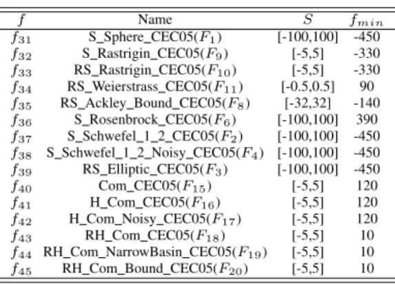
TEST FUNCTIONS OFf31TOf45CHOSEN FROM[41]
f Name S fmin
f31 S Sphere CEC05(F1) [-100,100] -450
f32 S Rastrigin CEC05(F9) [-5,5] -330
f33 RS Rastrigin CEC05(F10) [-5,5] -330
f34 RS Weierstrass CEC05(F11) [-0.5,0.5] 90
f35 RS Ackley Bound CEC05(F8) [-32,32] -140
f36 S Rosenbrock CEC05(F6) [-100,100] 390
f37 S Schwefel 1 2 CEC05(F2) [-100,100] -450
f38 S Schwefel 1 2 Noisy CEC05(F4) [-100,100] -450
f39 RS Elliptic CEC05(F3) [-100,100] -450
f40 Com CEC05(F15) [-5,5] 120
f41 H Com CEC05(F16) [-5,5] 120
f42 H Com Noisy CEC05(F17) [-5,5] 120
f43 RH Com CEC05(F18) [-5,5] 10
f44 RH Com NarrowBasin CEC05(F19) [-5,5] 10
f45 RH Com Bound CEC05(F20) [-5,5] 10
peer algorithms that are taken from the literature to compare with SLPSO in this paper.
The first algorithm is the cooperative PSO (CPSO-Hk) [44],
which is a cooperative PSO model combined with the original PSO. For this algorithm, we also use the same value for the “split factor” k = 6 as it was used in the original paper [44]. The second algorithm is the fully informed PSO (FIPS) [29] with a U-ring topology that achieved the highest success rate. The third algorithm is the comprehensive learning PSO (CLSPO) [25], which was proposed for solving multi-modal problems and shows a good performance in comparison with eight other PSO algorithms. The fourth peer algorithm is the adaptive PSO (APSO) [52], which adaptively tunes the values of η1,η2, and ω based on the population distribution
TABLE IV
PARAMETERS SETTINGS FORf3,f12,f13,f14,AND ROTATED AND
ROTATED SHIFTED FUNCTIONS
f Parameter values f3 yi= xi, |xi|<1/2, round(2xi), |xi| ≥1/2 f12 u(x, a, k, m) = k(x−a)m, x > a, 0, −a≤x≤a, k(−x−a)m, x <−a. m=10,M1−10(f13)=identity matrix,c1−10(f14) = 2
f13 g1−2= Sphere function,g3−4=Rastrigin function
f14 g5−6=Weierstrass function,g7−8=Griewank function
g9−10=Ackley function
biask= 100(k−1), k= 1,2, . . . ,10
f29 c= 100
f23–f28,f30 c= 2
TABLE V
CONFIGURATION OF THEINVOLVEDPSO ALGORITHMS
Algorithm Year Population Topology Parameter Settings SPSO[28] 2007 Local ring ω= 0.721,η1=η2= 1.193
CPSO-Hk[44] 2004 Cooperative multi- ω: [0.4, 0.9],η1=η2= 1.49
swarm approach k=6
FIPS[29] 2004 Local URing χ= 0.7298,Pc
i= 4.1
CLPSO[25] 2006 Comprehensive learning ω: [0.4, 0.9],η= 2.0
APSO[52] 2009 Global star ω: [0.4, 0.9],η1+η2: [3.0, 4.0]
with adaptive tuning TRIBES-D[8] 2009 Adaptive
FPSO[11] 2009 Adaptive ω: [0.4, 0.9],Pc
i= 4.0
JADE[53] 2009 An adaptive DE algorithmp=0.05,c=0.1 HRCGA[13] 2008 A real-coded GA PG=25%,NFG=200, NG M=400,N L F=5,N L M=100
G-CMA-ES[2] 2005 An ES algorithm Default settings in [2] APrMF[30] 2009 A memetic algorithm Default settings in [30]
in the fitness landscape to achieve different purposes, such as exploration, exploitation, jumping out, and convergence. The fifth peer algorithm is the standard PSO (SPSO) where the implementation can be downloaded at [28] (note that, this is a bit different from the one proposed in [5] and more widely used than the one in [5]). We chose this algorithm to investigate how SLPSO performs compared to the standard version of PSO. The sixth PSO algorithm is Frankenstein’s PSO (FPSO) [11], which is a composite PSO algorithm that combines a time-varying population topology, FIPS’s velocity
update mechanism, and a decreasing inertial weight. Since the number of total fitness evaluations is fixed for the experimental study in this paper, we used the suggestion by [11] to set the parameters in FPSO where a slow topology change schedule and an intermediate inertia weight schedule were used in this paper. The seventh peer algorithm, the TRIBES PSO algorithm [8], is also an adaptive PSO algorithm which can adaptively tune the number of particles needed and the population topol-ogy. The implementation of TRIBES PSO is provided at [28]. Note that the implementation of the TRIBES algorithm used in this paper is a simplified version of the paper [8].
Four non-PSO algorithms are also included in the com-parison with SLPSO. They are the JADE [53], HRCGA [13], APrMF [30], and G-CMA-ES [2] algorithms. JADE is an adaptive differential evolution algorithm with an optional external archive and HRCGA is a real-coded GA based on parent-centric crossover operators. We used the JADE with an archive in this paper since it has shown promising results compared with JADE without an archive in [53]. The param-eters p for the DE/current-to-pbest strategy and c for JADE were set to 0.05 and 0.1, respectively, as suggested in [53]. For the HRCGA algorithm, a combination of the global and local models were used where the number of female and male individuals for the two models were set to 200, 400 and 5, 100, respectively and the hybridization factor PG was set to
25%. APrMF [30] is a probabilistic memetic algorithm, which is able to analyze the probability of evolution or individual learning. By adaptively choosing one of the two actions, the APrMF algorithm can accelerate the search of global optimum. G-CMA-ES [2] is a covariance matrix adaptation (CMA) evolution strategy (ES) algorithm with re-start mechanism and increasing population size. For SLPSO, η was set to 1.496, Vmax was set to half of the search domain for each test
function, which can be seen from Table I and Table III, and the default parameter settings suggested in Section V-C (to be introduced in the following section) were used for all problems unless explicitly stated in this paper.
To fairly compare SLPSO with the other 11 algorithms, all algorithms were implemented and run independently 30 times on the 45 test problems. The initial population and stop criteria were the same for all algorithms for each run. The maximal number of fitness evaluations (T F es) was used as the stop criteria for all algorithms on each function. The pair of swarm size and T F es was set to (10, 50000), (20, 100000), (30, 300000), and (100, 500000) for dimensions 10, 30, 50, and 100, respectively. For TRIBES-D, the adaptive swarm size model was used where it begins with a single particle and adaptively decreases or increases the number of particles that are needed. The population size for the HRCGA algorithm and the APrMF algorithm was suggested by [13] and [30], respectively. Any other parameter settings of the 11 peer algorithms are based on their optimal configurations as suggested by the corresponding papers.
C. Performance Metrics
1) Mean Values: We record the mean value of the differ-ence between the best result found by the algorithms and the
TABLE VI
ACCURACY LEVEL OF THE45PROBLEMS
Accuracy level Function
1.0e-6 f1,f7,f9,f11,f12,f16,f18,f19
f21,f23,f26,f27,f29,f31,f35,f39 0.01 f2,f3,f4,f5,f6,f8,f10,f15,f17,f20,f22
f24,f25,f28,f30,f32,f33,f34,f36,f37,f38 0.1 f13,f14,f40,f41,f42,f43,f44,f45
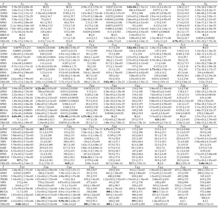
global optimum value over 30 runs on each problem, defined as: mean= 30 X k=1 (f(~x)−f(~x∗))/30 (13) where x and ~x∗ represent the best solution found by an algorithm and the global optimum, respectively.
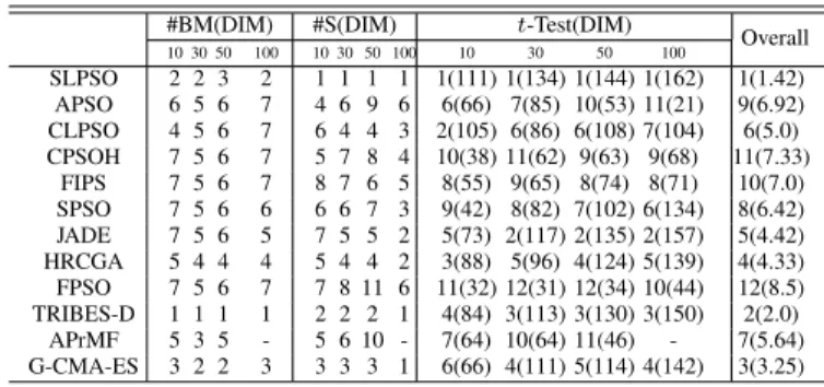
2) t-Test Comparison: To compare the performance of two algorithms at the statistical level, the two-tailed t-test with 58 degrees of freedom at a 0.05 level of significance was conducted between SLPSO and the peer algorithms. The performance difference is significant between two algorithms if the absolute value of thet-test result is greater than 2.0.
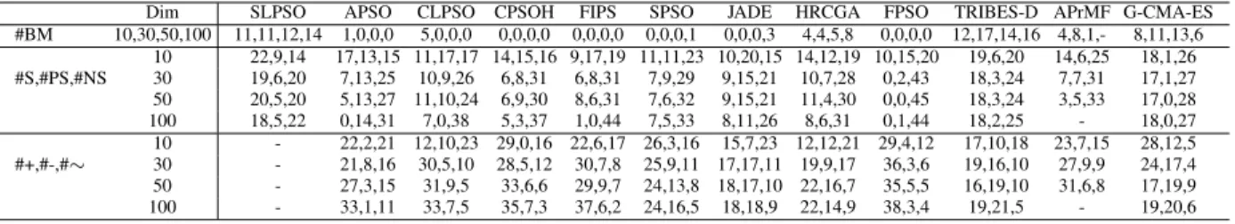
3) Success Rate: Another performance metric is the success rate, which is the ratio of the number of successful runs over the total number of runs. A successful run means the algorithm achieves the fixed accuracy level within the T F es fitness evaluations for a particular problem. The accuracy level for each test problem is given in Table VI. The accuracy levels for functionsf31-f45are obtained from [41] and the accuracy
levels of other functions are the same as used in [41], which were set according to the problem difficulty for all involved algorithms.
V. EXPERIMENTALSTUDY ONSLPSO
A. Self-Learning Mechanism Test
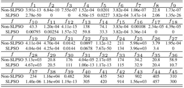
In order to investigate the level of effectiveness that the adaptive learning mechanism can bring to SLPSO, we carried out experiments on SLPSO with the adaptive learning mech-anism and SLPSO without the adaptive learning mechmech-anism (denoted Non-SLPSO) over all the test functions in 30 dimen-sions. For SLPSO, the default parameter settings were used. In Non-SLPSO, all the four operators have the same selection ratio of 0.25 during the whole evolutionary process. Table VII presents the results of SLPSO and Non-SLPSO on the 45 test functions.
Table VII shows that the result of SLPSO is much better than that of Non-SLPSO on 36 out of the 45 test problems. The reason to the result that SLPSO performs worse than Non-SLPSO on some problems is because the parameter values used were improper for those problems. This can be seen from the comparison of SLPSO with the default configurations and the optimal configurations in the next section where the performance of SLPSO with the optimal configuration is greatly improved. The comparison results show that the adaptive mechanism works well on most problems. It is also confirmed that different problems need different strategies to solve. To achieve the best performance, it is necessary to tune the selection ratios of the four operators so that the best strategy can effectively play its role.
TABLE VII
COMPARISON WITH RANDOM SELECTION FOR THE FOUR OPERATORS
REGARDING THE MEAN VALUE
f f1 f2 f3 f4 f5 f6 f7 f8 f9 Non-SLPSO 3.91e-13 6.84e-10 7.55e-07 1.52e-04 0.0201 3.82e-04 1.06e-07 22.8 1.73e-07
SLPSO 2.78e-50 0 0 4.50e-15 0.0227 3.82e-04 3.47e-14 2.06 1.35e-26 f f10 f11 f12 f13 f14 f15 f16 f17 f18 Non-SLPSO 43.3 1.20e-04 4.11e-15 138 74.1 3.83e-04 0.00108 2.34e-05 4.39e-05
SLPSO 0.00793 0.00254 1.57e-32 59.8 33.3 3.82e-04 3.36e-14 0 0 f f19 f20 f21 f22 f23 f24 f25 f26 f27
Non-SLPSO 4.11e-04 4.70e-04 0.0142 0.0897 1.12e-12 211 5.98e+03 3.79 1.95e-04 SLPSO 4.04e-04 4.25e-04 0.0144 0.0678 7.67e-50 134 3.96e+03 3.4 0
f f28 f29 f30 f31 f32 f33 f34 f35 f36 Non-SLPSO 5.13e+03 20.8 176 4.04e-05 2.17e-05 174 34.2 20.8 58.9 SLPSO 4.67e+03 20.5 111 1.00e-13 1.17e-13 115 32.9 20.4 10.7 f f37 f38 f39 f40 f41 f42 f43 f44 f45 Non-SLPSO 234 1.16e+04 0.482 304 435 543 902 405 310 SLPSO 1.40e-06 1.16e+04 1.19e-13 305 420 914 1.56e+03 457 300
TABLE VIII
SELECTED EXAMPLES OF EFFECT ON THE THREE PARAMETERS(Uf,Pl,
ANDM)INSLPSO
Uf f1 f6 f20 Pl f1 f6 f20 M f1 f6 f20
1 2.92e-32 7.9 35.5 0.05 1.74e-110 347 320 0 0.00817 0.295 0.138 3 1.41e-29 11.8 15.8 0.1 4.39e-128 205 138 0.1 0.00278 0.015 0.0176 7 1.10e-20 3.82e-04 11.8 0.3 5.01e-61 43.4 27.6 0.3 7.73e-04 0.0065 0.0076 10 3.81e-19 7.9 7.9 0.7 1.35e-26 3.95 11.8 0.7 7.83e-06 7.1e-04 0.0012 1 3.81e-19 7.9 7.9 1 3.81e-19 7.9 7.9
B. Parameter Sensitivity Analysis of SLPSO
There are three key parameters in SLPSO: the update frequency (Uf), the learning probability (Pl), and the number
of particles that learn from the abest position (M). To find out how the three key parameters affect the performance of SLPSO, an experiment on the parameter sensitivity analysis of SLPSO was also conducted on all the 45 problems in 30 di-mensions. The parameter of the number of particles that learn from the abestposition (M) is replaced by the percentage of the population size in this section. The default values of the three parameters were set to 10, 1.0, and 1.0, respectively. To separately test the effect of a particular parameter, we used the default values of the other two parameters. For example, to test the effect ofUf, we use a set of values forUf and the default
values for Pl (Pl= 1.0) andM (M = 1.0), respectively.
Three groups of experiments with Uf set to [1, 3, 7, 10],
Plset to [0.05, 0.1, 0.3, 0.7, 1.0], andM set to [0.0, 0.1, 0.3,
0.7, 1.0] were carried out separately. Table VIII shows the results on three example functionsf1,f6, andf20. Because of
the space limitation, the results of the other functions are not provided in this paper. From Table VIII, similar observation of the effect on the three parameters can be seen that the optimal value of each parameter for a specific problem does depend on the property of that problem.
Although we have an insight on how the three parameters affect the performance of SLPSO, the corresponding optimal value of each parameter above may not be the real optimal pa-rameter settings for a particular problem. It is difficult to obtain the real optimal parameter settings for a general problem for several reasons. First, we cannot test all the possible values of the three parameters as one of them is continuous, e.g.,Pl.
The value of M is population size dependent. Second, there may be relationships among the three parameters, i.e., they are not independent for SLPSO to achieve the best performance on a general problem.
In order to test whether the three key parameters of SLPSO
TABLE IX
COMPARISON OFSLPSOWITH OPTIMAL AND DEFAULT CONFIGURATIONS
IN TERMS OF MEAN VALUES
f f1 f2 f3 f4 f5 f6 f7 f8 f9 Optimal 6.16e-139 0 0 0 0.00173 3.82e-04 1.06e-14 0.0551 3.36e-71 Default 2.78e-50 0 0 4.50e-15 0.0227 3.82e-04 3.47e-14 2.06 1.35e-26 f f10 f11 f12 f13 f14 f15 f16 f17 f18 Optimal 7.45e-10 1.89e-05 1.57e-32 27 33.7 3.82e-04 1.23e-14 0 0 Default 0.00793 0.00254 1.57e-32 59.8 33.3 3.82e-04 3.36e-14 0 0 f f19 f20 f21 f22 f23 f24 f25 f26 f27
Optimal 1.48e-04 4.02e-04 0.00941 0.0298 3.22e-111 88.4 2.49e+03 0.249 0 Default 4.04e-04 4.25e-04 0.0144 0.0678 7.67e-50 134 3.96e+03 3.4 0 f f28 f29 f30 f31 f32 f33 f34 f35 f36 Optimal 1.98e+03 20.4 81.1 5.49e-14 9.28e-14 75.4 28.7 20.3 1.22 Default 4.67e+03 20.5 111 1.00e-13 1.17e-13 115 32.9 20.4 10.7 f f37 f38 f39 f40 f41 f42 f43 f44 f45 Optimal 4.86e-10 1.71e+03 5.68e-14 265 403 488 400 363 290 Default 1.40e-06 1.16e+04 1.19e-13 305 420 914 1.56e+03 457 300
TABLE X
OPTIMAL PARAMETER SETTINGS FOR THE45PROBLEMS
f f1 f2 f3 f4 f5 f6 f7 f8 f9 f10f11f12f13f14f15 Uf 3 1 1 1 3 1 1 1 3 1 10 1 1 1 1 Pl 0.1 0.05 0.1 0.05 0.05 0.05 0.05 0.1 0.1 0.1 0.7 0.3 0.3 0.1 0.05 M 1 0.7 0.7 0.7 0 0.1 0.7 1 1 1 1 1 0.1 0.3 0.1 f f16f17f18f19f20f21f22f23f24f25f26f27f28f29f30 Uf 7 1 1 7 1 1 1 7 10 3 1 1 3 1 7 Pl 0.05 0.7 0.1 0.05 0.05 0.05 0.05 0.1 0.05 0.05 0.05 0.3 0.05 0.05 0.05 M 1 1 1 0 0.1 0 0.7 1 1 0 0 1 0.1 1 0 f f31f32f33f34f35f36f37f38f39f40f41f42f43f44f45 Uf 10 7 10 1 1 10 3 10 7 3 3 1 3 1 10 Pl 0.05 0.3 0.05 0.05 0.05 0.1 0.1 0.05 0.05 0.05 0.1 0.1 0.05 0.1 0.3 M 1 1 0 1 1 1 1 0 1 0.3 0 0.1 0.3 0.3 1
are interdependent or not, further experiments were carried out based on the combination of the values given above for all the three parameters. The experimental results regarding the best results on each problem are summarized in Table IX and the corresponding optimal combinations of the three parameters for each problem are shown in Table X. It should be noted that we take the parameters of the optimal combinations as the real optimal configurations of SLPSO for each test problem even if they may not be the real optimal configurations.
Comparing the optimal configurations for each problem obtained in this section with the results in the above section, we can see that the three key parameters do have inter-relationship. Taking the Sphere function (f1) as an example,
the optimal combination of the three parameters are 3, 0.1, and 1 for Uf, Pl, and M, respectively, which are different
from the above experimental results where the corresponding optimal values are 1, 0.05, and 1, respectively. Therefore, there is probably no effective general rule that can be applied to set up the three parameters in SLPSO.
C. Parameter Tuning in SLPSO
The values of these three key parameters significantly affect the performance of SLPSO on most problems tested in this paper. To achieve the best performance for SLPSO, different optimal values of Uf, Pl, and M are needed on different
problems, which can be seen from the above experimental study on the parameters sensitivity analysis. The aim of this section is to suggest several approaches to adjusting the values of the three parameters for a general problem without manually tuning the parameters.
First, we present a general solution to set up the values of the update frequency (Uf) for SLPSO on all problems.
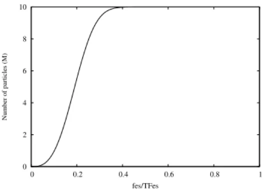
0 2 4 6 8 10 0 0.2 0.4 0.6 0.8 1 Number of particles (M) fes/TFes
Fig. 1. The number of particles that use the convergence operator at different iterations in a swarm of 10 particles.
Based on our previous work in [21], the optimal values ofUf
mainly distribute from 1 to 10 on most test problems in [21]. This information is very useful for SLPSO to set upUf for a
general problem. In order to use this information, we assign each particle with a different value of Uf instead of using the
same value ofUf for all particles. The value ofUf for particle
k is defined as follows:
Ufk= max(10∗exp(−(1.6·k/N) 4
),1) (14) whereNis the population size andUk
f is the update frequency
of particlek. By this scheme, the values ofUf of all particles
distribute from 1 to 10. As a result, it is possible that some particles may be able to achieve the optimal value of Uf for
different problems. Similar idea was implemented in CLPSO [25] to adjust the learning probabilityPc for each particle on
a general problem.
For the learning probability (Pl), we use the same setup
method as used for the update frequency where the learning probabilities of all particles distribute between 0.05 and 1.0, which is described as follows:
Plk= max(1−exp(−(1.6·k/N) 4
),0.05) (15) In order to reduce the risk of using improper values of Uf
andPl for a particular particle, we generate a permutation of
index numbers of particles every iteration and then update the values ofUfandPlfor each particle. As to how many particles
should use the convergence operator, we use the following formula:
M(f es) =N·(1−exp(−100(f es/T F es)3)) (16) where T F es is the total number of fitness evaluations al-lowed for a run. Fig. 1 shows the function relationship between M and f es. From Fig. 1, it can be seen that all particles initially do not use the convergence operator in order to focus on local search. However, to accelerate the convergence, the number of particles that use the convergence operator will gradually increase to the maximum value of 10 when the number of fitness evaluations reaches 40% of the total number of fitness evaluations. The main reason of using this particular method instead of using the selection ratio of the convergence operator to tune the value ofM lies in that we need to bring another new parameter of the maximum selection ratio for the convergence operator in order to achieve the objective. In
Algorithm 5 UpdatePar()
1: Create a permutation of index number;
2: UpdateUffor each particle by Eq. (14); 3: UpdatePlfor each particle by Eq. (15);
4: Calculate the number of particles using the convergence operator by Eq. (16);
5: Update related information of the four operators for each particle by Algorithm 3;
6: Calculate the inertia weightωby Eq. (17);
addition, the optimal value of the maximum selection ratio for different problems probably is different and unknown.
In SLPSO, the inertia weightω linearly decreases from 0.9 to 0.4 according to the following equation:
ω(f es) = 0.9−0.5∗f es/T F es (17) In order to show the effectiveness of these parameter tun-ing methods, comparison between the optimal configurations and the default configurations suggested in this section was conducted. The results are shown in Table IX. From the results, it can be seen that the performance of SLPSO with the default configurations is comparable to that with the optimal configurations on most test problems. However, this result also shows that it is necessary to further study how to effectively set up the parameters of SLPSO for general problems.
The parameter tuning equations used in SLPSO were de-veloped empirically from our experimental study based on the problems selected in this paper. Although these equations and the constants used in them, e.g., 1.6 in Eq.(14) and Eq.(15), may be not the optimal ones to set the values for the parameters of SLPSO, they were not randomly chosen but a result of a careful analysis. The analysis of all these equations is not discussed as it is not the main task of this paper. Here, we just provide some ideas of how to tune the parameters for SLPSO for general problems, and users can design their own methods to set the parameters for SLPSO. However, we would like to discuss some experience from our experimental study in terms of tuning the three key parameters in SLPSO. For the parameters Uf andPl, we should allow enough particles
to use the extreme values, e.g., 25% of total particles using the value of 0.05 or 1.0 forPl. Regarding M, it is important
that no particle learns from the abest position initially and the number of particles that learn from the abest position gradually increases until all particles learn from the abest position when the number of fitness evaluations reaches about 40% of total fitness evaluations. Although the parameter tuning methods were developed based on the problems used in this paper, they can also be used for new problems. These methods work well and the evidence can be seen from the comparison of SLPSO that uses these methods to set the parameters with other algorithms in Section VI. The update operations of these parameters in SLPSO are summarized in Algorithm 5.
D. Selection Ratios of the Four Operators
So far, although we have recognized that the adaptive learning mechanism is beneficial, it is not yet clear how the four operators in SLPSO would perform on a general problem. To answer this question, we analyze the behavior of each learning operator on some selected problems of 30 dimensions over 30 runs. To clearly show the learning behavior of the
0 0.1 0.2 0.3 0.4 0.5 0.6 0.7 0 50000 100000 selection ratios
fitness evaluations f1 (Sphere)
a b c d 0 0.1 0.2 0.3 0.4 0.5 0.6 0.7 0 50000 100000 selection ratios
fitness evaluations f2 (Rastrigin)
a b c d 0 0.1 0.2 0.3 0.4 0.5 0.6 0.7 0 50000 100000 selection ratios
fitness evaluations f11 (Schwefel_2_21)
a b c d 0 0.1 0.2 0.3 0.4 0.5 0.6 0.7 0.8 0 50000 100000 selection ratios
fitness evaluations f18 (S_Sphere)
a b c d 0 0.1 0.2 0.3 0.4 0.5 0.6 0.7 0.8 0 50000 100000 selection ratios
fitness evaluations f25 (R_Schwefel)
a b c d 0 0.1 0.2 0.3 0.4 0.5 0.6 0.7 0 50000 100000 selection ratios
fitness evaluations f45 (RH_Com_Bound_CEC05)
a b c d
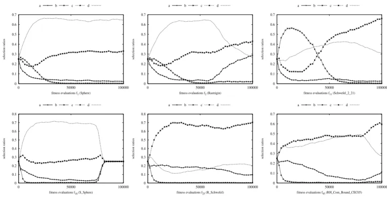
Fig. 2. Selection ratios of the four operators on six selected functions, wherea,b,c, andddenote the exploitation, jumping-out, exploration, and convergence operators, respectively.
four operators without impact from other factors, we allowed all particles to use the convergence learning operator through the whole run in this set of experiments. Fig. 2 only presents the results on six problems since similar observations can be obtained on other functions. From Fig. 2, several observations can be made and are described below.
First, the operators have very different performance on each specific problem and their performances also vary on different problems. On many problems, the best learning operator changes from the beginning to the end of evolution. For example, the best learning operator is the jumping-out operator (operatorb) for the Schwefel 2 21 function (f11) at
the early stage. However, its selection ratio decreases after
f es = 20000 until the end. On the contrast, the selection
ratio of the exploration operator (operatorc) increases and the exploration operator becomes the best learning operator after about 50000 evaluations. There is a period fromf es= 40000
tof es= 50000 where the convergence operator (operatord)
turns out to be the best learning operator. The exploitation op-erator (opop-eratora) may be not suitable for the Schwefel 2 21 function as its selection ratio decreases from the beginning and remains at a very low level till the end.
Second, for some functions, the best learning operator does not change during the whole evolution process, e.g., the convergence operator on the Sphere function (f1) and
the exploration operator on the R Schwefel function (f25).
The corresponding selection ratios remain at the highest level during the whole evolution process on these two functions.
In addition, the convergence status appears at the population level for the S Sphere function (f18). From the graph of
function f18, we can see that the selection ratios of the four
operators return to the initial state, where they almost have
the same value of 0.25. The convergence status shows only if none of the four learning operators can help particles to move to better areas. Of course, when a whole swarm converges to the global optimum, this phenomenon will show.
In general, we can get the following observations: 1) due to the advantages of the convergence operator discussed in Section III-E, particles get the greatest benefit from the con-vergence operator on functions f1, f2, and f18; 2) although
the jumping-out operator has the lowest selection ratio on most problems, it does help the search during a certain period on some problems, e.g.,f11; 3) particles always get benefit from
the exploration operator and even the largest benefit from it on some functions, e.g.,f25, andf45; 4) the exploitation operator
may work for a short period after particles jump into a new local area as its selection ratio never reaches the highest level. The results of this section confirm that different problems need different kinds of intelligence to solve them and that an adaptive method is needed to automatically switch to an appropriate learning operator at each evolutionary stage. We can also draw the conclusion that the individual level of intelligence works well for most problems.
VI. EXPERIMENTALSTUDY ONCOMPARISON WITH
OTHERALGORITHMS
A. Comparison Regarding Mean and Variance Values
In this section, experiments were conducted to compare SLPSO with 11 peer algorithms described in Section IV-B. Each algorithm was executed 30 independent runs over the 45 test problems in four dimensional cases, which are 10, 30, 50, and 100 dimensions, respectively, except the APrMF algorithm in 100 dimensions. The reason is that the program of APrMF