Working Paper No. 455
The Minskyan System, Part III:
System Dynamics Modeling of a Stock Flow–Consistent Minskyan
Model
By Eric Tymoigne
UMKC – Department of Economics June 2006
The Levy Economics Institute Working Paper Collection presents research in progress by Levy Institute scholars and conference participants. The purpose of the series is to
disseminate ideas to and elicit comments from academics and professionals.
The Levy Economics Institute of Bard College, founded in 1986, is a nonprofit, nonpartisan, independently funded research organization devoted to public service. Through scholarship and economic research it generates viable, effective public policy responses to important economic problems that profoundly affect the quality of life in the United States and abroad.
The Levy Economics Institute P.O. Box 5000
Annandale-on-Hudson, NY 12504-5000 http://www.levy.org
ABSTRACT
This is the last part of a three-part analysis of the Minskyan Framework. The paper presents a model that studies some of the features presented in Parts I and II. The model is Post-Keynesian in nature and puts a large emphasis on the role of conventions and the importance of the
financial side. In doing so, it provides an innovative way to determine aggregate investment and to introduce nonlinearities in the modeling of Minsky’s framework. This nonlinearity relies on the shifting property of conventions and the behavioral and psychological assumptions that they carry. Another specific characteristic of the model is that it is stock-flow consistent and
explicitly takes into account the amortization of principal and refinancing loans. All of the modeling is done by using system dynamics, a flexible but rigorous modeling tool that gives the modeler a good understanding of the dynamics of complex models.
JEL classifications: E5
The dynamics of the financial instability hypothesis are complex and varied. They represent tendencies, not automatic trends, which are triggered under specific conditions and can be partly dealt with by appropriate policies. Because of these multiple dynamics, it is very hard to grasp their implications for the behaviors of the economic system, and System Dynamics modeling is of a great help.
The following presents a Minskyan model combining two tools: System Dynamics and a stock-flow table. Based on the in-depth analysis of Minsky’s framework made in Part I and Part II, the model emphasizes the importance of conventional decision making for investment determination. Several dynamics are studied among which are the evolution of the normal and actual cash-flow margins over the cycle, the impact of the central bank, and the business cycle. The first part of the paper presents different elements of the model. The second part of the paper shows what the dynamics of specific elements are and under which conditions they generate the dynamics put forward by Minsky. The last part draws conclusions about the model.
1. THE MODEL
The basic model is a three-sector model with a household sector, a firm sector, and a banking sector, and with two different assets, capital assets and demand deposits. There are no secondary markets on which the ownership of capital assets is tradable, and there is no government sector (the central bank is added later but the Treasury is left aside).
The household sector consumes and saves in demand deposits; this sector does not invest and is not involved in any portfolio choices. In addition, workers are exclusively employed in the firm sector; the banking sector does not need any employees to perform its operations.
The firm sector is divided in two sub-sectors, the investment-good sector and the consumption-good sector, but the investment decision is made in common. Production occurs only on demand for the investment goods and is determined by expected demand for
consumption goods.
Banks provide loans and maintain a financial record of all economic transactions. Loans are created on demand providing that the firm sector meets the criteria set by banks to get loans. Banks determine the cost of external funds, that is, the maturity term and the interest rate of the loans. Like firms, they do not distribute any of their profit.
1.1. The Accounting Framework
Table 1 below presents the accounting framework of the basic model. The upper part of the table records the flow implications of the model, and the lower part presents the stock implications by presenting the balance sheet of each sector. The upper part is divided in two sub-sections, one that records the flows induced by income production and income distribution (both the income and balance-sheet operations of Minsky are there), and another part (based on the Flow of Funds analysis) that records the portfolio operations (i.e., changes in the balance sheets) induced by the preceding operations. For the firm and banking sectors, a distinction is also made between current account (i.e., flow impacts on the income statement) and capital account (i.e., flow impacts on the balance-sheet statement) because of the double impact of net profit.
The light gray column represents the flow implications on balance sheets, therefore, “+” and “–” in the NIPA table for this column have to be read, respectively, as sources and uses of funds. Changes in balance sheets that are represented in the NIPA table are changes in the assets and liabilities induced by the productive and distributive sides of the system. Changes recorded in the Flow of Funds table are changes in the financial side.1
The consistency of stocks and flows, that is the necessity for each stock and each flow to be recorded twice, is verified if the sum for all flows and all stocks, for each sector and across sectors, is zero. If the model does not generate this, it means that one important part of the model has not been taken into account. Appendix C gives an example taken from the model.
One important point to note is that the Flow of Funds table records net amounts; that is, the gross amounts of debts and demand deposits newly created net of the reflux of bank IOUs to the banking sector via the servicing of principal, and the amount of debts written off. Thus, the net change in the amount of debts is:
∆nL = ∆L – aL – zL
with ∆L the gross amount of loans (new debts), aL the amount of principal serviced, and zL the amount of debts written off.
Table 1: Stock and Flow Consistency
Flows
NIPA: Income Transactions Matrix
(+: Inflows, -: Outflows)
Sectors Households Firms Banks Balancing items Total flows
Current Capital Current Capital
Consumption -C +C 0 Investment +I -I 0 Sales [Y] Wage bill +W -W 0 Net profit -ΠnF +ΠnF -ΠnB +ΠnB 0 Interest on short-term loans -istLst +istLst 0 Interest on long-term loans -iltLlt +iltLlt 0 Financial balances +SH 0 +ΠnF – I 0 +ΠnB 0 0
Flow of Funds: Balance-sheet Transactions Matrix (Net Amount)
(+: Sources of Funds (lower assets/higher liabilities), -: Uses of Funds (higher assets/lower liabilities))
Demand deposits -∆nDDH -∆nDDF +∆nDD 0 Short-term loans +∆nLst -∆nLst 0 Long-term loans +∆nLlt -∆nLlt 0 Equity capital +zL -zL 0 Total sectors 0 0 0 0 0 Stocks Balance-Sheet Matrix (+: Assets, -: Liabilities)
Sectors Households Firms Banks Balancing items Total stocks
Current Capital Current Capital
Fixed capital +PKK -PKK 0
Demand deposits +DDH +DDF -DD 0
Debts -L +L 0
Balancing items -NWH -NWF -NWB +PKK 0
The gross amount of loans can be detailed more by making a difference between long-term and short-term debts. Then, we have:
∆Lst = ∆LW + ∆LREF
∆Llt = ∆LI
The gross amount of short-term loans depends on the amount of money necessary to pay the wage bill, and the amount of loans that have been granted to refinance positions. The gross amount of long-term debts depends on the amount of external funds needed by firms to fund investment. Thus, in total, in net terms we have:
∆nLst = ∆LW + ∆LREF – astLst – zstLst
∆nLlt = ∆LI – altLlt – zltLlt
Of course, the same is true for demand deposits, except for the writing-off which affects equity capital:2
∆nDD = ∆DD – aL
∆nEB = ΠnB – zL
∆nEF = ΠnF + zL
One can note, immediately, that short-term loans do not grow exclusively to finance productive economic activities, i.e., activities that contribute to the growth of national income. One can see also that there is no need for unproductive indebtedness other than refinancing to generate this phenomenon.
The rest of the accounting structure is pretty straightforward; for example, the national income identity is:3
C + I ≡ Y ≡ W + ΠnF + iL
One important thing to understand is, however, that ΠnF, the net profit of firms, does not
represent the amount of funds available for the funding of investment. Indeed, the net cash flow generated by net profit needs to be diminished by aL, which gives the amount of internal funds
available for investment:
ΠnF = ΠF – iL
2 This impact on equity assumes that all loans are unsecured loans and that banks do not provision for expected losses on bad loans. Adding secured loans would imply taking into account changes in the value of collaterals, which have a great impact on the willingness to lend.
3iL is the “net interest” component of national income: it does not include the net interest paid by the government to the private sector (it is included in personal income). Thus, in the model with a central bank, iHH – iAA, the
ΠIF = ΠnF – aL
Cash outflows induced by the amortization of debts are not part of the income account but part of the capital account. This shows the importance of the cash-flow analysis, ignored in the stock-flow table, because internal funds are determined by both income and capital
considerations. Therefore, one last important thing to take into account, in addition to the income (flow) and balance-sheet (stock) implications, are the cash-flow implications; the cash box condition will do that.
Finally, a point that is emphasized in Minsky’s theory is that the mismatch between assets and liabilities is due to a maturity differential, the loans granted being usually of shorter term than the gestation period of new capital assets. This is taken explicitly into account in the model in which the gestation period of new capital goods is assumed to be twice the maturity of long-term loans.
1.2. The Different Parts of the Model
The model contains a productive side and a financial side. The former explains how production, employment, consumption, investment, prices and profits are determined at the aggregate level. The latter side deals with the method through which economic activity is financed and funded: payment of investment, payment of cash commitments, and determination of the normal cash-flow margin. The distinction between the two sides is sometimes not clear-cut. For example, the level of aggregate profit is determined by the investment and saving decisions of economic agents, and the normal cash-flow margin directly affects the level of investment. However, as shown below, this distinction is essential even though it is usually ignored in models.
1.2.1. The Productive Side
In order to produce, the firm sector needs to employ people and so to pay wages; this payment must be financed. In the model, there are two sectors: the consumption sector and the
investment sector. Employment is derived from the amount of output produced O and a given average productivity of workers APL:
N = O/APL
Production is initiated differently in the consumption-good sector and in the investment-good sector. In the former, it is the level of expected profitable demand that determines
production, whereas investment goods are produced on demand. The level of expected profitable demand of consumption goods is determined as follows:
⎩ ⎨ ⎧ ≤ Π > Π = 0 ) ( if 0 0 ) ( if ) ( / ) ( ) ( C C C Cd E E P E N cwE O E
If profit from production is expected to be non-positive, then no production occurs; otherwise production depends on the expected level of employment and of price of consumption goods. The determination of the investment is explained by expectations concerning its funding structure:4 ⎩ ⎨ ⎧ ≤ > ∆ + Π = Is Id Is Id I IF I Is P P P P L E E O P if 0 if ) ( ) (
The determination of E(∆LI) has already been presented in Part II and is equal to:5
) ( ) ( ) ( ) ( ) ( a i E E cc cc E L E I + Π ⋅ ⎟⎟ ⎠ ⎞ ⎜⎜ ⎝ ⎛ Π Π ⋅ − = ∆
where cc (CC/П) is the flow leveraging ratio, E(cc) ≡ ccn is the normal flow-leveraging ration,
and E(ПIF) is based on an initial expectation of internal funds that is progressively modified by
the past level of internal funds. All this allows taking into account in the Post Keynesian
framework the importance of cash-flow and liquidity positions for investment decision. Fazzari, Hubbard, and Petersen (1988) have shown that these financial factors are central.
The level of aggregate profit of firms is determined by the Kalecki equation of profit which in the model is reduced to:6
ΠF = PIsOI – SW
4 Other solutions would be to run down cash balances or to augment capital so that P
IsOI≡I = ΠIF + ∆LI + α∆DD + ∆E. Here it is assumed that I = ΠIF + ∆LI. ∆E, addition to equity, usually entails a non-contractual (dividend on ordinary shares) or contractual increase in cash commitment (dividends on preferred stocks or any other forms of commitments) that depends on profits. Analytically ∆E can be considered conceptually equivalent to an increase in debt (Minsky 1975, 107; Toporowski 2000). The use of cash balance (α∆DD) also decreases the margins of security of units (or economy) and so is also conceptually equivalent to ∆LI (Minsky 1975, 108).
5 In the case of E(∆L
I), if Π is negative, this boosts the desired external funding of investment, which intuitively does not look appropriate. Thus, a boundary has to be put on Π and Q, and if they become negative, their value in the formula cannot go below zero. In fact the boundary has to be stricter and Π≥ 1 has to be imposed to avoid the unrealistic multiplicative effect for Π < 1.
where PIsOI is the investment level and SW is saving out of wage income.
The offer prices of consumer and investment goods are derived from the work done by Weintraub (1978) and Minsky (1986). More formally (knowing that C = PCQCd = c(wCNC +
wINI)) the price level in the consumption-good sector is:
LC C C LC C C C I I C AP w AP w N w N w c P ⎟⎟⋅ = ⋅ ⎠ ⎞ ⎜⎜ ⎝ ⎛ + ⋅ = 1 λ
The offer price of investment good, PIs, is determined by a given mark-up over unit labor cost in
the investment sector.
Finally, the difference between the demand price and the supply of investment goods is obtained by taking the equilibrium condition for wealth allocation:7
PIsK + DD = PIdK + mDD⇒PId – PIs = DD(1 – m)/K
The problem becomes, then, to explain how ccn is formed; that is, how cca and ccd are
determined. In order to do so, the financial side of the model has to be examined.
1.2.2. The Financial Side
The financial side of the model contains several important elements notably the determination of cash commitments that can be paid, and the determination of cca and ccd. In order to determine
the former, CC has to be explained and the cash-box condition, i.e., the cash-flow consistency, has to be established (firms cannot spend more money than they have).
a)Cash Commitments
The level of cash commitment is determined as follows:
CC = (i + a)L = (i + a)(Lst + Llt) = (i + a)(LW + LI + LREF)
There are two important elements here that are usually ignored in the literature: the amortization rate and the amount of debt resulting from refinancing loans (i.e., loans induced by the
incapacity to meet cash commitments). To simplify, only the interest payment of the debt service could be analyzed, but, as Minsky recognized, this is not a good approximation of the
7 Here we made a simplification relative to Minsky’s framework because what needs to be compared are P
Id and PI. The latter, the deliver price of investment goods, includes the discounted valued of the cash commitments induced by borrowing external funds to fund investment. More strictly, one should also include the discounted value of
financial cost when debts are short-term debts because the amortization of the principal becomes important (Caskey and Fazzari 1986):
In fact, if the financial contracts are sufficiently short, then the cash payments on financial contracts can exceed the total quasi rents. (Minsky 1975, 84).
One of the tendencies of the Minskyan analysis is for the amortization rate to go up during a period of prolonged expansion, even if interest rates are fixed.
The amount of loans resulting from pure financial considerations (speculation,
refinancing operations, or any other), is also important to take into account because those have a tendency to grow in level and proportion over a period of prolonged expansion. In the model, there is no speculation because there are no financial markets: capital assets are illiquid.
b)Conventions Regarding the Cash-Flow Margin
The simplest explanation of changes in ccn concerns the firm sector. In the firm sector,
ccd has an initial value at time 0. This value is progressively corrected over time by a correction
factor:
∑
= + = T t t d dT cc cc 1 0 νwhere νt represents the correction factor. The latter can be negative or positive depending on the difference between the actual and expected structure of funding. For example, if ∆LI/(ΠIF + ∆LI)
< E(∆LI)/(E(ΠIF) + E(∆LI)), it means that the firm sector has a lower proportion of external
funding than expected, and this leads to an upward change in ccd: The desired cash-flow margin
goes down.
Bankers have a more complex method of correction because not only do they adjust their
cca progressively, but they also change the basic cca from which they do progressive
corrections. Let us note cca the basic flow leveraging ratio with cca = cca0 at time 0. The method
of correction in the banking sector is thus:
⎩ ⎨ ⎧ = + =
∑
= 2 condition if 1 condition if 2 1 x x cc cc cc a T t t a aT τ τ τ ωLiterally, this means that the current acceptable cash-flow margin is the sum of the prevailing basic acceptable cash-flow margin and a degree of correction. The degree of correction ωt
depends on the rate of profit of banks and the proportion of debts not serviced. The conditions that lead to a shift in cca are related to the same factors plus the proportion of refinancing loans
that have been granted by banks.
One important difference between the banking sector and the firm sector concerns their degree of optimism as reflected in the correction factors νt and ωt. The bankers are the skeptics of the game, so they have a downward (upward) bias in the correction of their acceptable flow leveraging ratio (cash-flow margin). On the contrary, the upward correction of ccd is stronger
than the downward correction. All this tries to capture the psychological idea that entrepreneurs are more sensitive to good results than bankers. In the end, the normal flow-leveraging ratio, ccn
is determined as follows:
ccn = min(ccd, cca)
c)The Cash Box Condition
This condition is central to the Minskyan system so one has to be sure that it is well modeled, and that it is able to determine well the amount of cash commitments that can and cannot be serviced. In terms of cash commitments, the following condition must be true in order for all cash commitments on debts to be serviced:8
CCt ≤ Πt + αDDFt + ∆LREFt
This condition states that, in order for the cash commitments to be paid, there must be enough funds available either from new sources of cash, i.e.,gross profit and/or refinancing loans, or from accumulated past net cash inflows, i.e., from dishoarding. If this is not the case, part of CC
cannot be serviced. In order to be sure that this condition was always respected, several simulations were run to verify that the difference between CC and the sum of serviced and not serviced cash commitments is nil, and to be sure that the amount of cash commitments serviced
was never superior to Π + αDDF + ∆LREF.
The servicing of the cash commitments is done in a predefined way: interest payments are serviced first and short-term debts are serviced before long-term debts. Therefore, the first
payment to meet is the interest payment on short-term debts, then comes the interest payment on long-term debts, followed by the principal payments. At each step, one has to make sure that there is enough funds to serve part or the whole amount due, if this is not the case, writing-off occurs for an amount related to the amount of principal not serviced.
1.2.3. Shortcomings
If the model is able to take into account some important characteristics of the Minskyan analysis like the importance of conventions and of the cash box condition, it leaves aside other important components that will not be developed here. In addition, some rough simplifications have been made.
The first element that has been left aside is the determination of interest rates and
maturities; related to this is the fact that the propensity to hoard is also given and left
unexplained. As stated earlier, the Minskyan analysis does not require that interest rates go up during the boom, but the maturity of debts should have a tendency to decrease via the heavier weight of refinancing loans and the higher optimism of economic agents. The growth of cash commitments, of course, does not need to be based on any change in the unit cost of external funds, so assuming constant unit costs is, from this point of view, not important. There is, however, one source of increase in the cost of external funds via the central-bank rate, and, as shown above, this is a central cause of increase in interest rates that Minsky recognized.
One way to explain the interest-rate structure would be to assume that short-term rates reflect an expectation of the central-bank rate and that long-term rates are a function of expected short-term rates and expected long-term rates (Robinson 1953; Kahn 1954). However, in the model, there are no financial markets, so interest rates cannot be determined in this way.
Another problem concerns the productive side of the model. There is no explanation of production and its effect on the investment decision. This will have an impact on the investment demand, either by affecting the needs to replace the capital that wore out, or by affecting net investment because, for example, the rate of utilization of the capacity of production is higher than what is considered a normal rate of utilization (Lavoie 1992). Related to this problem is the fact that investment in the model is a common decision in the firm sector; the investment
their actual needs of capital goods.9 All this reflects the awkwardness of not distinguishing between funding decisions and investment decisions. Both are important and should be treated independently. The model emphasizes the financial side of the matter to show its importance; this side being usually either ignored or considered as an irrelevant “veil.”
Another shortcoming in the model is the fact that the criteria used to determine cca are
partly fixed. One may think that these threshold values change over time with economic condition and that it is not only the difference between actual level and these thresholds that matters for the change in cca.
Another shortcoming concerns the lack of any distribution of dividends or interest income to households. One could think that firms and banks distribute part of their gross profit to households, and that this would affect consumption, inflation, growth, and employment, but this is not taken into account here. A later model could easily develop this part of the model, which is not essential for the main argument.
One shortcoming that puts limits on the applicability of the model is that it assumes that the external cost (both in terms of interest rate and maturity term) is variable for the whole outstanding debt. Thus, a change in interest rates or maturity terms affects all the existing debts and not only new debts. Following Minsky, this implies that the model can never take into account a hedge situation.
Finally, the model does not take into account the role of the Treasury, which is essential for the determination of interest rates (both long- and short-term interest rates) and for the amount of reserves available in the system. The public deficit is also a central element that stabilizes the aggregate macroeconomic profit and that can be used to fight inflation (Lerner 1943; Bell 2000; Wray 1998, 2003, 2004b).
2. SIMULATIONS
Several simulations are presented below that analyze specific dynamics of the Minskyan framework and check under which condition they are verified. In order to do so, two different
models are used: one in which the unit cost of external funds (i + a) is fixed, and another one in which the central bank affects short-term rates.
2.1.1. The Role of the State of Expectations: Normal Ratios and Profit Expectations
The state of expectations, as reflected in expectation of profits and given criteria of decisions used to determine the riskiness of economic projects, is central to the dynamics of the Minskyan model. If one starts with the normal cash-flow margin, we know that it depends on the
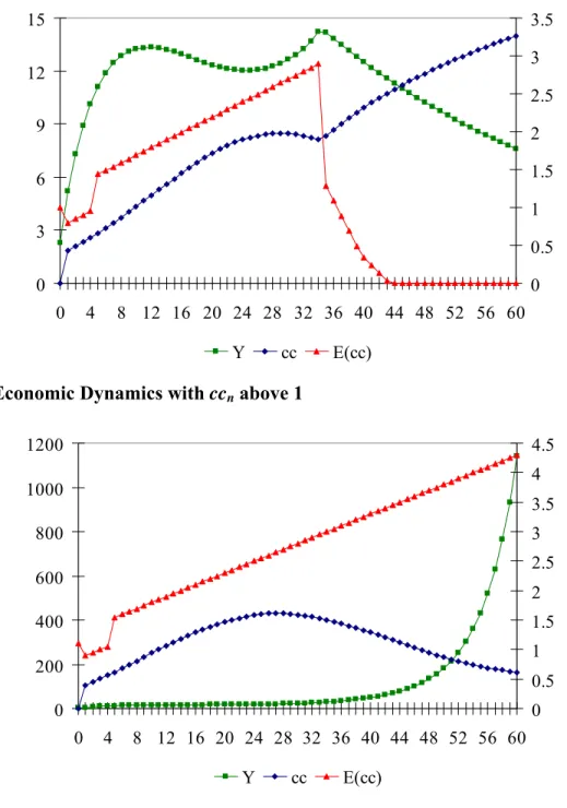
convention existing in the firm sector and the bank sector about the appropriate cash-flow margin. Depending on the initial value of those two norms of cash-flow margins, the economy can go from a boom to a depressed economic situation as shown in Figures 1 and 2.
Figure 16 shows what happens when ccn is equal to 1 or is below this value (sales are on
the left axis). The economy can never recover from its depressed situation if there is no external intervention or shock (lower cost of external funds, fiscal deficit, etc.). Figure 2 reaches the same conclusion for a boom economy. If the initial value of ccn is above 1, the economy grows
forever. Note that this is in contradiction with the conclusions of Minsky and consistent with Lavoie (1997); in Figure 2 the expansion never stops and is transformed into an inflationary boom: Firms are never in financial difficulty, their financial situation always strengthens (cc
tends toward 0), they never have to ask for any refinancing loans. However, this assumes that the cost of external funds stays unchanged over the expansion period, that there is no fiscal policy that tries to contain the growth of the economy, and, of course, that no other external forces emerge to influence ccn. As stated earlier, if there is a barrier to the non-inflationary
growth of income via tight fiscal and monetary policies, the expansion period is overturned. This will be simulated below.
Figure 1: Economic Dynamics with ccn below 1 0 3 6 9 12 15 0 4 8 12 16 20 24 28 32 36 40 44 48 52 56 60 0 0.5 1 1.5 2 2.5 3 3.5 Y cc E(cc)
Figure 2: Economic Dynamics with ccn above 1
0 200 400 600 800 1000 1200 0 4 8 12 16 20 24 28 32 36 40 44 48 52 56 60 0 0.5 1 1.5 2 2.5 3 3.5 4 4.5 Y cc E(cc)
If one takes the initial expectations of gross profit, the same results are obtained. Given ccn, a
change in the initial E(П) leads to either an explosive expansion or a permanently depressed economy. In this private economic system, given all other constant values, there are no forces that generate an economic recovery and so no economic business cycle exists.
All the preceding shows that initial economic conditions are crucial for the dynamics of the economic system. If one goes further and includes shocks on ccn and E(П) at another time
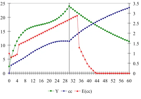
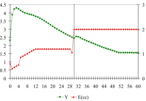
than time 0, then the economy can go from a period of depression (expansion) to a period of boom (depression). Figure 3 shows what happens when the state of expectations is shifted by -$68 at quarter 30.
Figure 3: Effect of a Shift in E(П) on the Dynamics of the System
0 5 10 15 20 25 0 4 8 12 16 20 24 28 32 36 40 44 48 52 56 60 0 0.5 1 1.5 2 2.5 3 3.5 Y cc E(cc)
One can see that a shift that is high enough, generates a shift in the economic dynamics from a boom to a depressive situation (sales are on the left axis) even if ccn > cc. This is so because,
due to the shift in E(П), the latter becomes negative, and it is assumed that if this is the case, the desired external funding E(∆LI) is zero whatever the relation between ccn and cc.
The state of expectations, as represented here by Q and ccn, has dramatic effects on the
behavior of the economic system. This importance of expectations is not a particularity of the Minskian or Keynesian frameworks, as Kregel (1977) noted. However, the importance of
conventional expectations is a particularity of the two preceding approaches. The expectations
are not based on a ‘true’ model but on mental models that try to explain the future performance of the economy. Individuals know they can be systematically wrong. One implication of this is that the comparison of past expectations and current results (the exante/expost distinction) is not
the way expectations mainly affect the dynamics of the economic system. The comparison of current expectations and current state of affairs if far more important.
2.1.2. Cost of External Funds
Minsky stated that over the boom period, the unit cost of external funds may have a tendency to rise, either because of higher interest rates or amortization rates. Because of the nature of the first model, this cannot be verified by looking only at the private banking system. The basic model can, however, look at the impact of an exogenous increase in the cost of external cost for different economic situations.
Two situations are presented below; one in which the economy is in a favorable
expectational environment, and one in which expectations are pessimistic. In both cases, a shock on the cost of external funds is imposed at quarter 30 in the form of higher interest rates (+1000 basis points) and lower maturity terms (cut in half).
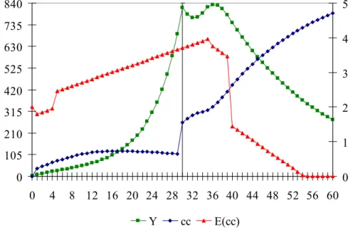
In the first economic situation, presented in Figure 4, the initial conditions concerning expectations of gross profit and normal cash-flow margin are favorable to the emergence of a boom, and without any shock, the economy would grow indefinitely and financial fragility would never occur whatever the refinancing acceptance rate (because no refinancing loans is ever needed). Before the shock, the normal leveraging ratio goes up while the actual flow-leveraging ratio goes down toward zero. However, after the shock, even if the economy still grows, the normal and actual leveraging ratios have their tendency that changes. The downturn occurs at quarter 36, and without any additional shock to reverse the tendency, sales go down forever.
Figure 4: Shock on the Cost of External Funds with an Optimistic State of Expectations 0 105 210 315 420 525 630 735 840 0 4 8 12 16 20 24 28 32 36 40 44 48 52 56 60 0 1 2 3 4 5 Y cc E(cc)
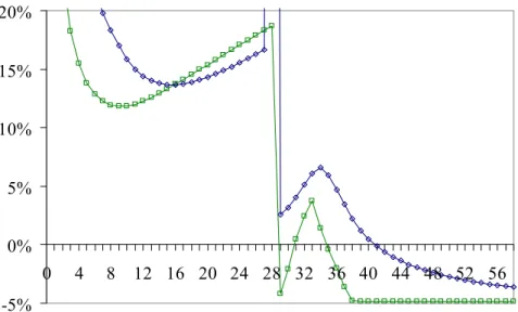
Another way to look at this is in terms of the rate of growth of cash commitments
relative to the rate of growth of sales. As shown in Figure 5, before the shock, the rate of growth of CC is lower than the rate of growth of sales, whereas after the shock the reverse occurs. This first simulation is, therefore, able to take into account some of the conclusions of Minsky even if the cost of external funds is exogenous.
Figure 5: Rate of Growth of Sales versus Rate of Growth of Cash Commitments -5% 0% 5% 10% 15% 20% 0 4 8 12 16 20 24 28 32 36 40 44 48 52 56
rate of growth of sales rate of growth of cash commitments
In the second situation, the economy starts with a state of expectations that is
pessimistic, which is materialized by higher initial desired and acceptable cash-margins. Figure 6 represents what happens in the economy before and after a shock (sales are on the left axis) for which maturity terms are doubled, and interest rates are decreased close to zero. No shock on the cost of external funds, whatever its size (very low interest rates or very high maturity terms), can change the dynamics of the system. Thus, if the economy is depressed, using the cost of external funds to try to revive the economy is ineffective. This is so in the model because, whatever the cost of external funds, the firm sector is never able to fully service its debts, which depresses its expectations and those of banks. The essential conclusion from this second simulation is that using interest rates or maturity terms to revive the economy will not work if expectations are not affected positively so that income can grow. One suspects that if a fiscal policy that aimed at sustaining private profits were introduced, the economy would be able to go out of its depressed situation.
Figure 6: Shock on the Cost of External Funds with a Pessimistic State of Expectations 0 0.5 1 1.5 2 2.5 3 3.5 4 4.5 0 4 8 12 16 20 24 28 32 36 40 44 48 52 56 60 0 1 2 3 Y cc E(cc)
The next step is, then, to try to endogenize this increase in the cost of external funds and the possibility that the rate of growth of cash commitments might be lower than the rate of growth of sales, which will be done below. It will be shown that the central bank may have a large role to play in this increase. However, before looking at the role of the central bank, some other important characteristics of the model have to be simulated.
2.1.3. Speed of the Simplification Process
In the Minskyan analysis, a depressed laissez-faire economic system with a high level of debts will not recover until the simplification process is terminated, that is, until most of the non-performing outstanding debts are eliminated from the system so that CC is brought down to a reasonable level relative to Π.10 This simplification process leads to a period of large
disinvestments. The longer the period of simplification, the longer it takes for the recovery to proceed. On the contrary, the shorter the simplification period, the faster the liquidity of economic agents is restored.
10 The problem is, however, that, in the process of simplification, Π goes down as well as cc
n. A decrease in CC, therefore, may not be sufficient to restore economic growth.
A simulation was done to look at the implications of different speeds of simplification. In the model, the writing-off of debts depends on the amount of principal not serviced
multiplied by a constant factor that reflects the speed of simplification. By default, the
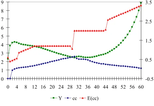
multiplicative factor is set to one, that is, the amount of debts written-off is equal to the amount of principal payments not serviced. A higher speed always leads to a faster recovery. In Figure 7, the economy starts in a depressed economic situation, and it is assumed that there is a positive shock on the normal cash-flow margins of +20 in quarter 30. By itself, this shock is not able to provide a durable expansion.
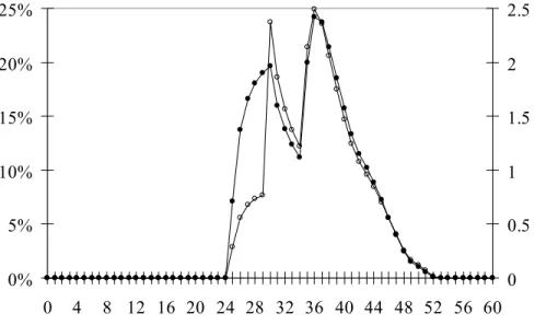
The amount of debts written-off grows but is never enough to remove the burden of cash commitments as shown in Figure 8. However, by multiplying the speed of the writing-off by 2 (i.e., by adding 1 to the parameter “speed of simplification”) in quarter 30, the economy first has a period of recovery and then starts to take off. This is shown in Figure 9. The expansion really occurs only after quarter 45 when, as shown in Figure 10, the simplification process is close to be finished. Before that, the amount of debts written-off is higher than in Figure 8, and this amount decreases rapidly as the amount of bad outstanding debts decreases.
Figure 7: Effect of Higher ccn with no Change in the Speed of Simplification
0 0.5 1 1.5 2 2.5 3 3.5 4 4.5 0 4 8 12 16 20 24 28 32 36 40 44 48 52 56 60 0 1 2 3 Y E(cc)
Figure 8: Debts Written-Off and Not Serviced 0% 10% 20% 30% 40% 50% 60% 0 4 8 12 16 20 24 28 32 36 40 44 48 52 56 60 0 1 2
percentage of debts not serviced total debts written off
Figure 9: Effect of Higher ccn with a Doubling in the Speed of Simplification
0 1 2 3 4 5 6 7 8 9 0 4 8 12 16 20 24 28 32 36 40 44 48 52 56 60 -0.5 0.5 1.5 2.5 3.5 Y cc E(cc)
Figure 10: Effect of Higher Speed of Simplification 0% 5% 10% 15% 20% 25% 0 4 8 12 16 20 24 28 32 36 40 44 48 52 56 60 0 0.5 1 1.5 2 2.5
percentage of debts not serviced total debts written off
From the two preceding simulations, one can conclude, as one would have expected, that cleaning accumulated debts from balance sheets helps the recovery and expansion to happen. If debts of firms are left in the balance sheets of banks, the recovery may never happen, whatever the willingness of firms and banks to invest, because the firms cannot face their cash
commitments.
2.1.4. Delay of Gestation and Maturity of Debts
One important point in the Minskyan framework is that there is a mismatch in the maturity of assets and liabilities. The higher the mismatch, the higher the fragility of the economy. This can actually be simulated in the model by changing the relation between the gestation period of investment goods and the maturity of long-term loans.
By default, the gestation period is set twice as long as the maturity of long-term loans. Figure 11 shows a period of depressed economic situation and financial weakening. Given everything else, if the gestation period is made equal to the maturity term of long-term loans, then the economy takes an expansionary path that rapidly transforms into a boom. This is shown in Figure 12. This effect depends also, however, on other factors like the state of expectation of
the economy. The economy may actually not start to expand. Nonetheless, by equalizing both maturity periods, the economy reaches a higher level of GDP.
Figure 11: Economic Situation Given the Gestation Period of Investment Goods
0 3 6 9 12 15 0 4 8 12 16 20 24 28 32 36 40 44 48 52 56 60 0 0.5 1 1.5 2 2.5 3 3.5 Y cc E(cc)
Figure 12: Gestation Period Equal to the Maturity of Long-Term Loans
0 1000 2000 3000 4000 5000 6000 7000 8000 9000 10000 11000 0 4 8 12 16 20 24 28 32 36 40 44 48 52 56 60 0 0.5 1 1.5 2 2.5 3 3.5 4 4.5 Y cc E(cc)
2.1.5. Monetary Policy
The last simulation looks at the impact of monetary policy. In order to do so, the basic model has to be modified to introduce the intervention of the central bank. It is assumed that the central bank sets the short-term rate on the advances that it grants to banks, and that the short-term rate on private loans is set by private banks via a mark up over the central-bank rate.11 In the real world, banks need to borrow central bank IOUs in order to be able to clear their positions among each other, and to meet reserve requirements. Thus, even if reserve requirements are nil, there is still a need for central bank IOUs (Fullwiler 2004; Lavoie 2005). In the model, banks need central-bank IOUs only to meet their reserve requirements. If reserve requirements are positive, then, in the model, the higher the reserve-requirement ratio, the lower the profit of banks, and so the lower is their cca.
Banks receive an interest rate on the deposits they held at the central bank. By default, it is assumed that the interest rate on advances and the interest rate on reserves are equal. The main tool of the central bank is the rate on advances; the other one just adjusts to it. It is, then, necessary to explain how the rate on advances is set. Several different rules to determine the rate of interest could be used; by default, the model assumes that the central bank reacts only to expected inflation. T T T 1 1 1 π 2 π) ( if π π) ( if π π) ( if 03 . 0 01 . 0 01 . 0 > > < ⎪ ⎩ ⎪ ⎨ ⎧ + + − = − − − E E E i i i i At At At At
Of course, in doing all this, one has to make sure that all the accounting constraints are met in terms of cash flow, income, and balance sheet. The stock-flow table is presented in appendix D and the cash-flow constraint for banks was easy to verify.
Several interesting results come out of the simulation of the model with monetary policy; among them are that some Minskian tendencies are endogenously generated by the model. In the following, two main simulations are presented, the impact of monetary policy on the business cycle and on interest rates, and the role of the amount of refinancing loans granted by banks to firms existing in the economy.
a) The Monetary Policy, Business Cycle, and Interest Rate
One of the central results, well known to economists, is that the central bank interest rate has an asymmetrical effect on the economy. If increasing interest rates can lead to a recession, it is, in the model, impossible to bring a recovery by decreasing interest rates even to zero. The source of the recovery must come from other sources like a shift in convention or a
simplification process. During the boom period, the central bank increases its interest rate because it expects inflation to go above its targeted inflation (which is set at 7% by default).12 This increase in the central bank interest rate affects the short-term rates on private loans, which affects the cash commitments due and the profitability of firms and banks, and so the normal margins of safety. A higher short-term interest rate results in higher financial fragility of the firms, i.e., lower cash-flow margin. This higher fragility affects the normal cash-flow margin which, through its shift, is, as shown in Figures 13 and 14, the direct cause of the recession. The abrupt decrease in E(cc) is generated by the growing proportion of debts that is not serviced as shown in Figure 15. This leads to an abrupt revision of expectations. As one can see, the proportion of debts not paid is zero until late in the period of expansion.
Another result that comes from the preceding Figure is that a situation in which the growth of cash commitments is superior to the growth of sales is endogenously generated. This results from the growing interest rate on short-term loans and reproduces pretty well the tendencies that Minsky put forward. It is possible to go back to recovery, but only after an extremely long process of simplification as shown in Figure 16.
12 Of course, the higher the inflation target, the more the economy growth can go on because short-term interest rates do not grow as steadily.
Figure 13: Central Bank Policy and Business Cycle 0 1000 2000 3000 4000 5000 6000 7000 8000 0 10 20 30 40 50 60 70 80 90 100 110 120 0% 5% 10% 15% 20% 25%
Y central bank rate on advances
Figure 14: Effect of Increasing Interest Rates
0 1000 2000 3000 4000 5000 6000 7000 8000 0 10 20 30 40 50 60 70 80 90 100 110 120 0 1 2 3 4 5 Y cc E(cc)
Figure 15: Debt Servicing and Economic Growth -10% 0% 10% 20% 30% 40% 50% 60% 0 10 20 30 40 50 60 70 80 90 100 110 120
percentage of debts not serviced rate of growth of sales
rate of growth of cash commitments
The recovery occurs because, with the simplification process, the amount of debts decreases and the capacity to meet cash commitments increases. This leads to a loosening of the normal cash-flow margin because of the loosening of the acceptable cash-flow margin: ccn goes
up. There are three picks for the percentage of debts not serviced; each of them represents a business cycle even if the scale of sales does not permit the reader to see it clearly. As shown in Figure 17, when ccn becomes high enough, the economy recovers.
It is, therefore, possible to have an expansion, recession, stagnation and recovery process that is generated endogenously via the introduction of monetary policy. However, the central bank is inefficient in bringing the recovery by acting on interest rates. Indeed, in the preceding, the recovery will occur only when the simplification process is close to being finished, and, as Minsky recognized, this can be one way to “manage” the system.
Figure 16: Simplification Process and Economic Recovery 0 1500 3000 4500 6000 7500 9000 0 20 40 60 80 100 120 140 160 180 200 704 724 744 764 784 804 824 844 864 884 904 924 944 964 984 0% 10% 20% 30% 40% 50% 60% 70%
Y percentage of debts not serviced
Figure 17. Normal and Actual Cash-Flow Margin
0 0.5 1 1.5 2 2.5 3 3.5 4 4.5 5 0 20 40 60 80 100 12 0 14 0 16 0 18 0 20 0 70 4 72 4 74 4 76 4 78 4 80 4 82 4 84 4 86 4 88 4 90 4 92 4 94 4 96 4 98 4 cc E(cc)
b) Monetary Policy when Refinancing Loans Are Granted
In the preceding simulations, it was assumed that the amount of refinancing loans granted by the private banking system was nil by default. This assumption is quite ad hoc, and even illogical, because if ccn is superior to one, it means implicitly that banks agree to grant
refinancing loans. However, for the sake of the simulations, it was assumed that the refinancing acceptance rate was zero. Thus, if firms could not pay their cash commitments, banks just wrote off a multiple of the principal due out of debts, and interest payments not serviced generated a cut in the profit of banks. In the following, it is assumed that the refinancing acceptance rate is equal to one. One immediate implication of this is that the rate of profit of banks is increased as shown in Figure 18. This necessity for banks to grant loans in order to allow firms to pay interest services was put forward by Wray (1991). Granting or not granting refinancing loans has, therefore, a large influence on the banking system.
Figure 18: Profitability of Banks and Refinancing Rate
0% 5% 10% 15% 20% 25% 30% 35% 0 4 8 12 16 20 24 28 32 36 40 44 48 52 56 60 rate of profit of banks (refinancing acceptance rate = 100%) rate of profit of banks (refinancing acceptance rate = 0%)
Another implication, shown in Figure 19, is that, while previously cash commitments could not increase for any other reasons than those related to the financing and funding of production given in the unit cost of external funds, they are now free to go up for reasons unrelated to the preceding ones. The rate of growth of CC now changes much faster and with higher amplitude when refinancing needs exist. In addition, the rate of growth of cash
commitments is much higher than the rate of interest. This is so for two reasons; first, the amortization rate is higher in the total amount of debts because of the short-term nature of refinancing loans, and second, the amount of cash commitments that cannot be met increases a lot, leading to an increase in the amount of refinancing loans. Figure 20 shows that, depending on the refinancing acceptance rate, the proportion of short-term debts changes a lot.
Figure 19: Effect of a Refinancing Rate of 100% on the Growth of CC
-5% 10% 25% 40%
0 4 8 12 16 20 24 28 32 36 40 44 48 52 56 Rate of growth of CC (Refinancing acceptance rate = 100%) Rate of growth of CC (Refinancing acceptance rate = 0%)
These Figures have the same initial economic conditions as Figures 28 to 32 except for the refinancing rate. One can, therefore, conclude that an economy with a high proportion of short-term loans is far more delicate to manage via interest-rate changes. Indeed, higher interest rates can rapidly increase the cost of the whole outstanding debts as short-term debts are rolled over, and lower interest rates may be inefficient in reducing the growth of cash commitments if
the growth of the latter is related to other reasons than the cost of loans. Another conclusion is that it does not take a high rate of acceptance for refinancing for short-term loans to become a very high proportion of outstanding debts.
Figure 20: Proportion of Short-Term Debts
0% 20% 40% 60% 80% 100% 0 4 8 12 16 20 24 28 32 36 40 44 48 52 56 60 "proportion of short-term debts" (refinancing acceptance rate = 100%) "proportion of short-term debts" (refinancing acceptance rate = 75%) "proportion of short-term debts" (refinancing acceptance rate = 50%) "proportion of short-term debts" (refinancing acceptance rate = 25%) "proportion of short-term debts" (refinancing acceptance rate = 0%)
By intuition, it seems reasonable to think that an economy in which the proportion of refinancing loans is high will grow at a slower path. Indeed, short-term refinancing loans add a burden on the economy by increasing the amount of cash commitments without stimulating the productive side of the economy. This is actually what happens in the model, as shown in Figure 21. However, the effect of different refinancing acceptance rates can be non-linear: higher rates may lead to higher economic growth given the unit cost of external funds. This result is possible because cca is affected by both the amount of debts not serviced and the amount of refinancing
loans granted: higher refinancing loans is bad for cca but helps to improve the servicing of debts,
which is good for cca. In this context, the manipulation of interest rates by the central bank is
Figure 21: Sales for Different Refinancing Context 0 105 210 315 420 525 630 735 840 945 0 4 8 12 16 20 24 28 32 36 40 44 48 52 56 60 Y (refinancing acceptance rate = 100%)
Y (refinancing acceptance rate = 0%)
3. CONCLUSION
The preceding exercise allows us to reach several conclusions in terms of Minsky’s theory and in terms of monetary policy. In terms of the former, one can first see the practicality of System Dynamics; it allows to detect some dynamics that otherwise are hard to figure out. The most important result is that Minsky’s financial instability hypothesis is verified endogenously if one includes a central bank that uses interest rates to try to manage the economy. Without the latter, the model endogenously generates dynamics that are opposite to the financial instability
hypothesis and side with Lavoie’s (1997) concerns that the hypothesis may not generate automatic tendencies. However, one has to recognize that even Minsky recognized this: “The existence of profit opportunities does not necessarily mean that fragile financing patterns will emerge immediately” (Minsky 1986, 211). Part II reviews in details and which condition fragility may occur. Other important elements that have been verified are the importance of maturity matching and the role of the simplification process in a free-market economy. Matching the maturity of assets and liabilities is extremely important for the stability and the dynamism of the economic system. If liabilities have a shorter maturity than assets, they have a tendency to accumulate faster and, once debt is overwhelming, a simplification process is
necessary before any expansion can occur. The simplification process cleans balance sheets of bad debts and allows economic agents to start over. All this shows the importance of the financial side of capitalist economic system; it affects the behavior of the rest of the system.
In terms of monetary policy, the preceding has several important implications. The first, most obvious one, is that interest-rate policies are ineffective and promote business cycles. The central bank should thus abandon this tool or even any other fine-tuning activities and
concentrate on other goals. The central goal that comes out of the model is financial stability: the central bank should promote the liquidity and stability of the system. The model suggests that this can be done by promoting maturity matching and the creation of financial instruments that are perfectly adapted to the needs of borrowers. The central banks should also take an active part in the definition of the normal margins of safety. The latter are pure conventions and there is no reason to assume that the central bank does not know anything about what a reasonable margin is. On the contrary, it can complement that private assessment of the normality by a public assessment that is detached from profitability considerations, and that takes into account the macroeconomic impacts of economic activities. The central bank can also be involved in the management of financial fragility by shortening the simplification process (or eliminating it altogether if conditions require it). If the central bank, or another governmental institution, took the lead in the speed of simplification by accepting to buy private debts so as to remove them from the balance sheet of private banks (instead of having banks writing them off), it would help in bringing the recovery. In the end, therefore, the best policy to implement is to let the central bank interest rate permanently at a low level (why not 0%?) so that no additional disturbance to the payment system are added: financial stability is the only goal that central banks have been able to manage successfully from their creation, so they should concentrate on this goal and improve its management.
REFERENCES
Bell, S. 2000. “Do taxes and bonds finance government spending?” Journal of Economic Issues, 34 (3): 603-620.
Caskey, J. and S. Fazzari. 1986. “Macroeconomics and credit markets.” Journal of Economic
Issues, 20 (2): 421-429.
Fazzari, S., R. G. Hubbard, and B. Petersen. 1988. “Financing constraints and corporate investment.” Brookings Papers on Economic Activity, 1, 141-195.
Fullwiler, S. T. 2004. “Setting interest rates in the modern money era.” Center for Full Employment and Price Stability, Working Paper No. 34.
Kahn, R. F. 1954. “Some notes on liquidity preference.” Manchester School of Economic and
Social Studies, 22 (3): 229-257. Reprinted in Kahn, R. (ed.) Essays on Employment and
Growth, 72-93. Cambridge: Cambridge University Press, 1972.
Kregel, J. A. 1977. “On the existence of expectations in English Neoclassical economics.”
Journal of Economic Literature, 15 (2): 495-500.
Lavoie, M. 1992. Foundations of Post Keynesian Economic Analysis. Aldershot: Edward Elgar. _________. 1997. “Loanable funds, endogenous money, and Minsky’s financial fragility
hypothesis.” In Cohen, A. J., H. Hagemann, and J. Smithin (eds.) Money, Financial
Institutions, and Macroeconomics, 67-82. Boston: Kluwer Nijhoff.
_________. 2005. “Monetary base endogeneity and the new procedures of the asset-based Canadian and American monetary systems.” Journal of Post Keynesian Economics 27 (4): 689-709.
Lerner, A. P. 1943 “Functional finance and the federal debt” Social Research, 10: 38-51.
Reprinted in Colander, D. (ed.) Selected Economic Writings of Abba L. Lerner, 297-310. New York: New York University Press, 1983.
Minsky, H. P. 1975. John Maynard Keynes. Cambridge: Cambridge University Press. _________. 1986. Stabilizing an Unstable Economy. New Heaven: Yale University Press. Robinson, J. V. 1953. The Rate of Interest and Other Essays. London: Macmillan.
Toporowski, J. 2000. The End of Finance. London: Routledge.
Weintraub, S. 1978. Capitalism’s Inflation and Unemployment Crisis. Reading, Massachusetts: Addison-Wesley.
Wray, L. R. 1991. “The inconsistency of Monetarist theory and policy.” Economies et Sociétés, 25 (11-12), MP 8: 259-276.
_________. 1998. Understanding Modern Money. Vermont: Edward Elgar.
_________. 2003. “Functional finance and US government budget surpluses in the new
millennium.” In Nell, E. J. and M. Forstater (eds.) Reinventing Functional Finance
Transformational Growth and Full Employment, 141-159. Northampton: Edward Elgar.
_________. 2004. “Conclusion: The credit money and state money approaches.” In Wray, L. R. (ed.), Credit and State Theories of Money, 223-262. Northampton: Edward Elgar.
APPENDIX A
Figure A2 represents the productive side of the system and is used to determine the level of aggregate profit. Figure A3 explains offer prices and calculates aggregate sales and the inflation rate. Figure A4 determines the expected quantity of consumption goods consumed. Figure A5 is the heart of the dynamics of the model and determines the private demand for investment (OId).
Figure A6 shows how the desired and normal flow-leveraging ratios are determined. Figure A7 determines the acceptable flow-leveraging ratio. Figure A8 shows how cash commitments are determined and how they can be met out of gross profit, refinancing and dishoarding. Figure A9 explains how the funding of investment is done and Figure A10 represents the cash box
condition and determines what proportion of cash commitments can be met. Figure A2: Employment, Production, and Profit
Consumption goods
new capital goods
consumption goods sold wage bill in C-sector consumption expenditure investment expenditure Capital assets gross profit in I-sector WAGE RATE IN I-SECTOR WAGE RATE IN C-SECTOR saving by household AVERAGE PRODUCTIVITY OF LABOR IN I-SECTOR AVERAGE PRODUCTIVITY OF LABOR IN C-SECTOR MARGINAL PROPENSITY TO CONSUME wage bill in I-sector gross profit in C-sector DEPRECIATION RATE <private investment demand>
total wage bill
total gross profit of firms production of consumption goods depreciation employment in I-sector employment in C-sector GESTATION PERIOD OF INVESTMENT GOODS consumption expenditure by households net profit of firms
<total interest servicing on long-term debts>
<total interest servicing on short-term debts>
<MATURITY TERM ON LONG-TERM LOANS>
gross profit in C-sector available to meet cash
commitments gross profit in I-sector available to meet cash
commitments investment expenditure in C-sector investment expenditure in I-sector Value of capital assets <offer price of investment goods> <offer price of consumer goods> INITIAL PRODUCTION OF CAPITAL GOODS <expected quantity demanded of consumption goods>
Figure A3: Offer Prices, Inflation and Sales
sales
<consumption expenditure>
<investment
expenditure> previous sales rate of growth of
sales <Time>
offer price of consumer goods
mark up over labor cost in C-sector previous offer price rate of inflation offer price of investment goods MARK UP OVER LABOR COST IN I-SECTOR <wage bill in C-sector> <wage bill in I-sector> <MARGINAL PROPENSITY TO CONSUME> <employment in C-sector> <employment in I-sector> <AVERAGE PRODUCTIVITY OF LABOR IN C-SECTOR> <WAGE RATE IN C-SECTOR> <WAGE RATE IN I-SECTOR> <AVERAGE PRODUCTIVITY OF LABOR IN I-SECTOR> quarterly factor
Figure A4: Determination of the Expected Quantity of Consumption Goods Demanded
LENGTH OF EXPECTATION IN C-SECTOR expected consumption expenditure expectations of gross
profit in C-sector expected offer price ofconsumption goods consumer goods><offer price of INITIAL EXPECTED OFFER PRICE expected profitable quantity demanded of consumption goods <WAGE RATE IN
C-SECTOR> <WAGE RATE INI-SECTOR> <MARGINAL PROPENSITY TO CONSUME> <AVERAGE PRODUCTIVITY OF LABOR IN C-SECTOR> INITIAL EXPECTATION OF EMPLOYMENT IN C-SECTOR expected employment in C-sector INITIAL EXPECTATION OF EMPLOYMENT IN I-SECTOR expected employment in I-sector <employment in
Figure A5: Determination of Quantity of Investment Goods Demanded
private investment demand
expected internal funds
desired external funds for investment funding actual flow leveraging ratio asset price differential PROPENSITY TO HOARD <Capital assets> <total gross profit of firms> <total cash commitments on debts> expected gross profit
<Total deposits held by the firm sector>
DELAY OF ADJUSTMENT OF EXPECTATION OF PROFIT <amortization rate on long-term loans> <INTEREST RATE ON LONG-TERM LOANS> INITIAL INTERNAL FUNDS EXPECTATIONS expected initial
cash commitment <Time> INITIAL GROSS
PROFIT EXPECTATIONS
total gross profit included in decision maximum value of the
flow leveraging ratio
<TIME STEP> <internal funds> <offer price of investment goods> <normal flow leveraging ratio>
<quarterly factor> expected internal funds
available for investment funding
Figure A6: The Desired and Normal Cash-Flow Margin
normal flow leveraging ratio desired flow leveraging ratio INITIAL FLOW LEVERAGING RATIO DESIRED proportion of external funding expected proportion of external funding <long-term loans to C-sector> <long-term loans to
I-sector> <desired external fundsfor investment funding>
difference between expected and actual external funding
degree of correction for firms DELAY IN
RECORDING DIFFERENCE
previous desired flow leveraging ratio
<Time> <Internal funds in C-sector
available for investment> <internal funds in I-sectoravailable for investment>
<acceptable flow leveraring ratio> UPWARD CORRECTION DOWNWARD CORRECTION
<expected internal fund available for investmen
funding>
UPWARD CORRECTION IF DIFFERENCE IS ZERO
Figure A7: The Acceptable Cash-Flow Margin
acceptable flow leveraring ratio
new basic acceptable flow leveraging ratio <refinancing loans granted to C-sector> <refinancing loans granted to I-sector> total refinancing loans granted
<total debts not serviced> <total debts serviced> percentage of debts not serviced degree of correction for banks <Total debts of firms> proportion of refinancing loans <Time> previous acceptable flow leveraging ratio INITIAL FLOW LEVERARING RATIO ACCEPTABLE DELAY IN ADJUSTING INITIAL RATIO BY BANKS <Total debts of firms> rate of profit of banks
Total loans granted by the banking system
TRP1 TRP2
TPDNS1 TPDNS2 TPRL1 TPRL2
<net profit of banks>
<quarterly factor> <Time> <quarterly factor>
UPWARD CORRECTION FOR BANKS FOR BASIC
CCa UPWARD CORRECTION FOR BANKS DOWNWARD CORRECTION 1 FOR BANKS DOWNWARD CORRECTION 2 FOR BANKS DOWNWARD CORRECTION 2 FOR BANK FOR BASIC CCa
DOWNWARD CORRECTION 1 FOR BANK FOR BASIC CCa
Figure A8: Cash Commitments
Long-term liabilities of C-sector amortization of long-term debts of C-sector long-term loans to C-sector <wage bill in C-sector>
interest payment due on long-term debts by
C-sector
cash commitments
on debts in C-sector commitments on debtstotal cash on debts in I-sectorcash commitments amortization of long-term debts of I-sector long-term loans to I-sector INTEREST RATE ON LONG-TERM LOANS MATURITY TERM ON LONG-TERM LOANS amortization rate on long-term loans
interest payment due on long-term debts by I-sector Short-term liabilities of C-sector amortization of short-term debts of C-sector short-term loans to C-sector Short-term liabilities of I-sector amortization of short-term debts of I-sector short-term loans to I-sector MATURITY TERM ON SHORT-TERM LOANS amortization rate on short-term loans <wage bill in I-sector>
interest payment due on short-term debts by
C-sector
INTEREST RATE ON
SHORT-TERM LOANS interest payment due onshort-term debts by I-sector additional needs of cash to
meet cash commitments in C-sector
additional needs of cash to meet cash commitments in
I-sector
<gross profit in C-sector>
<gross profit in I-sector>
principal payment due on short-term debts by
C-sector principal payment due on long-term debts by
C-sector
principal payment due on long-term debts by I-sector
principal payment due on short-term debts by I-sector Long-term liabilities of I-sector REFINANCING ACCEPTANCE RATE refinancing loans granted to C-sector <REFINANCING ACCEPTANCE RATE> refinancing loans granted to I-sector writing-off of short-term debts of C-sector writing-off of short-term debts of I-sector writing-off of long-term debts of I-sector writing-off of long-term debts of C-sector
actual dishoarding to face cash commitments in
C-sector <Demand deposits
of C-sector>
refinancing loans necessary to meet cash commitments
in C-sector
actual dishoarding to face cash commitments in
I-sector refinancing loans necessary
to meet cash commitments in I-sector
<Demand deposits of I-Sector>
SPEED OF
SIMPLIFICATION SIMPLIFICATION><SPEED OF
<SPEED OF SIMPLIFICATION> <SPEED OF SIMPLIFICATION> <servicing on principal on short-term debts by I-sector> <servicing of principal on short-term debts by C-sector> <servicing of principal on long-term debts by C-sector> <servicing of principal on long-term debts by I-sector> <external funds necessary to
fund investment in the C-sector>
<external funds necessary to fund investment in the
I-sector>
Figure A9: Funding of Investment
external funds necessary to fund investment in the
C-sector
internal funds in I-sector internal funds in
C-sector
external funds necessary to fund investment in the
I-sector
<cash commitments paid by C-sector>
<cash commitments paid by I-sector>
Internal funds in C-sector available for investment
internal funds in I-sector available for investment
internal funds
additional funds necessary to fund investment in
I-sector additional funds necessary
to fund investment in C-sector <gross profit in C-sector> <gross profit in I-sector> <investment expenditure in C-sector> <investment expenditure in I-sector>
Figure A10: Cash Box Condition
Demand deposits of C-sector inflows to C-sector outflows from C-sector Demand deposits of I-Sector inflows to I-sector outflows from I-sector Total deposits
held by the firm sector <consumption expenditure> <wage bill in C-sector> <wage bill in I-sector>
<interest payment due on long-term debts by
C-sector> <principal payment due
on long-term debts by C-sector>
<principal payment due on short-term debts by
C-sector>
<principal payment due on long-term debts by
I-sector>
<principal payment due on short-term debts by
I-sector> <interest payment due on
short-term debts by C-sector>
<interest payment due on long-term debts by
I-sector>
<interest payment due on short-term debts by
I-sector> <investment
expenditure>
loans granted to
C-sector loans granted toI-sector
<wage bill in
C-sector> <wage bill in
I-sector> <refinancing loans granted to C-sector> servicing of principal on short-term debts by C-sector servicing of principal on long-term debts by C-sector servicing of interest on long-term debts by C-sector servicing of interest on short-term debts by C-sector servicing of principal on long-term debts by I-sector servicing on principal on short-term debts by I-sector servicing of interest on long-term debts by I-sector servicing of interest on short-term debts by I-sector
principal due not serviced by C-sector
interest due not serviced by C-sector
principal due not paid
by I-sector serviced by I-sectorinterest due not
total principal not serviced total interest not
serviced <actual dishoarding to face cash commitments
in C-sector>
<refinancing loans granted to I-sector>
<actual dishoarding to face cash commitments in I-sector> cash commitments paid by C-sector cash commitments paid by I-sector Demand deposit of households inflows to house hold sector outflows from household sector
<total wage bill> <consumption expenditure> <gross profit in C-sector
available to meet cash commitments>
<gross profit in I-sector available to meet cash
commitments> <REFINANCING ACCEPTANCE RATE> <REFINANCING ACCEPTANCE RATE> <external funds necessary to
fund investment in the C-sector>
<external funds necessary to fund investment in the
I-sector> <investment expenditure in C-sector> <investment expenditure in I-sector>
APPENDIX B