The nonparametric analysis of interval-censored failure time data

(1)

THE NONPARAMETRIC ANALYSIS OF

INTERVAL-CENSORED FAILURE TIME DATA

A Dissertation

Presented to

the Faculty of the Graduate School

University of Missouri

In Partial Fulfillment

Of the Requirements for the Degree

Doctor of Philosophy

by

RAN DUAN

Dr. (Tony) Jianguo Sun, Dissertation Supervisor

(2)

The undersigned, appointed by the Dean of the Graduate School, have

examined the dissertation entitled

THE NONPARAMETRIC METHODS FOR THE

ANALYSIS OF INTERVAL-CENSORED DATA

presented by RAN DUAN

A candidate for the degree of Doctor of Philosophy

and hereby certify that in their opinion it is worthy of acceptance.

Dr. (Tony) Jianguo Sun

Dr. Nancy Flournoy

Dr. Subharup Guha

Dr. Jing Qiu

(3)

ACKNOWLEDGEMENTS

I owe my deepest gratitude to my esteemed advisor Dr. (Tony) Jianguo Sun for his generous support and help, wonderful guidance and endless patience, which enable me to complete this work and obtain the Ph.D degree. His continual encouragement and instruction lead me to a good start of my research life.

I extend my gratitude to my advisory committee members: Dr. Nancy Flournoy, Dr. Subharup Guha, Dr. Jing Qiu and Dr. Davis Wade for their insightful comments and suggestions on my work. Special thanks are due to Dr. Hui Zhao and Dr. Yanqing Feng for their helpful academic discussion and help.

I also want to express my deep gratitude to all faculty who taught me classes and assisted me in various ways during my course studies. I would also like to mention my special appreciation to Dr. Larry Ries for helping me to be a better instructor.

I want to thank our great staff Judy , Tracy and Kathleen for plenty of help. I would like to take this opportunity to extend many thanks to my fellow graduate students for making the department a strong one and I will always treasure the friendship and appreciate the help of friends here at Mizzou.

I am deeply indebted to my family, especially my parents, Tiansheng Zhu and Xiaochun Duan, for their unselfish love and support throughout my life. Its their company and care make my life so happy and wonderful.

(4)

List of Tables

2.1 Estimated Size and Power Based on Simulated Data from Exponential

Distribution . . . 99

2.2 Estimated Size and Power Based on Simulated Data from Gamma Dis-tribution . . . 100

2.3 Results on the Analysis of AIDS Clinical Trial . . . 101

3.1 Empirical Power and Size for Exponential Distribution . . . 102

3.2 Empirical Power and Size for Gamma Distribution . . . 103

3.3 Empirical Size for Exponential Distribution. . . 104

4.1 Simulation Result for Estimation of β. . . 105

(8)

List of Figures

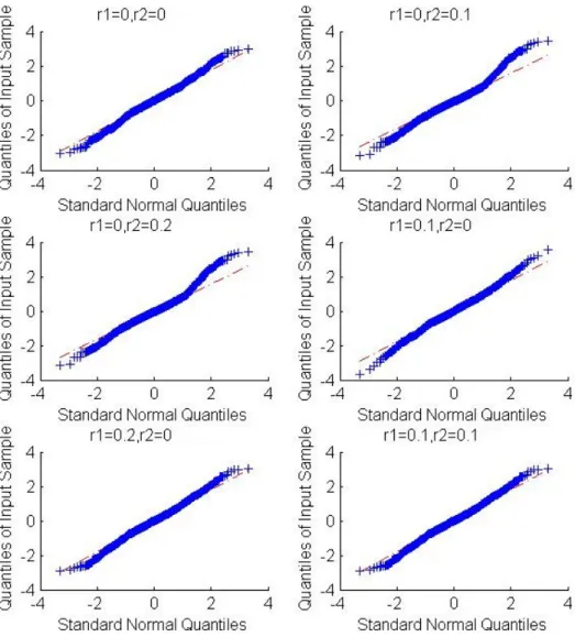
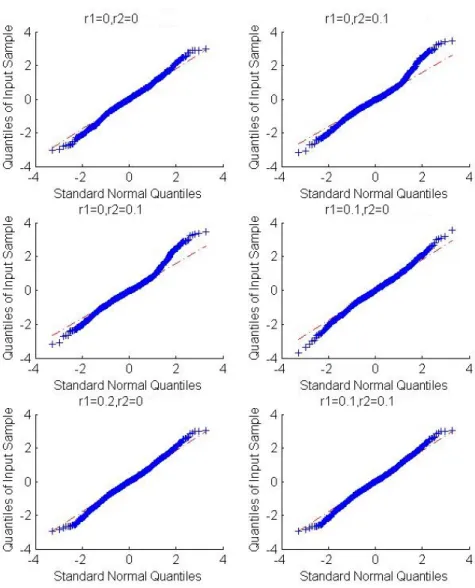
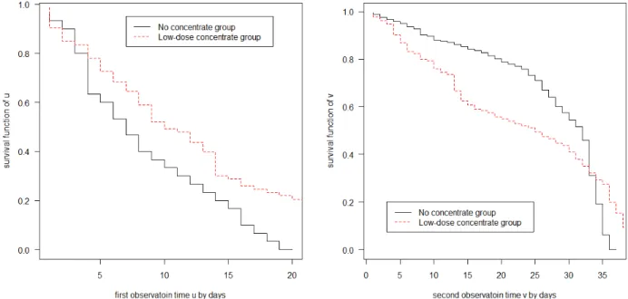
3.1 QQ-plot of Test Statistic for Exponential Distribution . . . 106 3.2 QQ-plot of Test Statistic for Gamma Distribution . . . 107 3.3 Kaplan-Meier estimate of survival function . . . 108

(9)

THE NONPARAMETRIC METHODS FOR THE

ANALYSIS OF INTERVAL-CENSORED FAILURE TIME

DATA

Ran Duan

Dr. (Tony) Jianguo Sun, Dissertation Supervisor

ABSTRACT

By interval-censored failure time data, we mean that the failure time of interest is observed to belong to some windows or intervals, instead of being known exactly. One would get an interval-censored observation for a survival event if a subject has not experienced the event at one follow-up time but had experienced the event at the next follow-up time. Interval-censored data include right-censored data (Kalbfleisch and Prentice, 2002) as a special case.

(10)

time studies such as clinical trials. For interval-censored failure time data, a few non-parametric test procedures have been developed. However, due to the strict restrictions of existing nonparametric tests and practical demands, some new nonparametric tests need to be developed.

This dissertation consists of four parts. In the first part, we propose a new class of test procedures whose asymptotic distributions are established under both null and alternative hypotheses, since all of the existing test procedures cannot be used if one intends to perform some power or sample size calculation under the alternative hypoth-esis. Some numerical results have been obtained from a simulation study for assessing the finite sample performance of the proposed test procedure. Also we applied the proposed method to a real data set arising from an AIDS clinical trial concerning the opportunistic infection cytomegalovirus (CMV).

The second part of this dissertation will focus on the nonparametric test for interval-censored data with unequal censoring. As we know, one common drawback or restric-tion of the nonparametric test procedures given in the literature is that they can only apply to situations where the observation processes follow the same distribution among different treatment groups. To remove the restriction, a test procedure is proposed, which takes into account the difference between the distributions of the censoring vari-ables. Also the asymptotic distribution of the test statistics is developed by counting process and martingale theory. For the assessment of the performance of the procedure,

(11)

a simulation study is conducted and suggested that it works well for practical situa-tions. An illustrative example from a study aiming to investigate the HIV-1 infection risk among hemophilia patients is provided.

The third part of this dissertation deals with the regression analysis of multivari-ate interval-censored data with informative censoring. Multivarimultivari-ate interval-censored failure time data often occur in the clinical trial that involves several related event times of interest and all the event times suffer interval censoring. Different types of models have been proposed for the regression analysis ( Zhang et al.(2008); Tong et al.(2008); Chen et al.(2009); Sun (2006)). However, most of these methods only deal with the situation where observation time is independent of the underlying survival time completely or given covariates. In this chapter, we discuss regression analysis of multivariate interval-censored data when the observation time may be related to the underlying survival time. An estimating equation based approach is proposed for re-gression coefficient estimate with the additive hazards frailty model and the asymptotic properties of the proposed estimates are established by using counting processes. A major advantage of the proposed method is that it does not involve estimation of any baseline hazard function. Simulation results suggest that the proposed method works well for practical situations.

Finally, we will talk about the directions for future research. One is about the nonparametric test for interval-censored data with informative censoring. The other is

(12)

(13)

Chapter 1 Introduction

1.1 Data Structure

1.1.1 Interval-Censored Data and Censoring Mechanism

Researchers working with survival data often face with issues associated with in-complete data, especially censoring issues. One important type of censored data is called interval-censored data. By interval-censored data, we mean that study subjects are not under continuous observation. As a result, the survival times could not be observed exactly and one can only observe a time interval within which the event has occurred. Exact, right-censored and left-censored failure time data are special cases of interval-censored data. The exact failure time data occur when the censoring in-terval is reduced to a single point and inin-terval-censored data become right-censored data or left-censored data when the right boundary of the interval is infinity or the left

(14)

boundary is zero.

Interval-censored data occur in all kinds of areas, for instance, epidemiology, finance, social science, etc.. One real example comes from an oncology phrase III trial for breast cancer. In its statistical analysis plan, cancer progression time was predetermined as the secondary end point. During the trail, patients needed to visit the physician periodically in order to take the treatment therapy and the visiting times of each breast cancer patient were recorded, which was a periodic discontinuous observation process. Therefore, we only knew that the progression time of a breast cancer patient fell into a time interval, which was from the last visiting time with no cancer progression to the first visiting time with cancer progression.

There are three types of interval-censored data. Case I interval-censored data (Groeneboom and Wellner, 1992) , which also known as current status data, refer to the situation where each study subject only has one observation time and the failure time is either left-censored or right-censored. One commonly used notation of current status data is

{C, δ=I(T ≤C}, (1.1)

where C denotes the observation time and δ is the censoring indicator (Sun 2006). Current status data often occur in demographical studies. For example, the ages of patients with respect to the incidence of a disease, of which the exact incidence times are hard to measure.

(15)

situ-ation that a time interval (L, R) instead of the exact failure time has been observed for a study subject. Here L is the lower boundary and R is the upper boundary of the interval. One way to present interval-censored data is

{U, V, δ1 =I(T ≤U), δ2 =I(U < T ≤V), δ3 = 1−δ1−δ2}, (1.2)

where U and V represent observation processes. Here U and V are two random variables satisfyingU ≤V andδis the censoring indicator (Sun, 2006). A more general situation is called Case K interval-censored data (Schick and Yu, 2000), which assume that each study subject has K observation points. The failure time falls in one of the

K + 1 intervals and K is an random variable. Then the observation information can be presented in the form of

{K, Uj, δj =I(Uj−1 < T ≤Uj), j = 1, . . . , K, U0 = 0}. (1.3)

The third type is doubly censored data (Sun, 1995), which occur under the situation that the objective of a clinical trial involves two related events. Then each individual has two event times and both of them are interval-censored. A common source of doubly censored failure time data is disease progression studies. For example, in a clinical trial, researchers are interested in tumor progression time as well as failure time for patients. Both of them are measured by the visiting time of patients. Therefore, doubly censored data have been collected at the end of the study.

(16)

1.1.2 Informative Censoring and Unequal Censoring

One common assumption of interval-censored data is that the observation process and event time are independent, which could be violated in practice. For example, a patient may withdraw from the study because the tumor grows too fast. Thus early withdraw may indicate a sooner death than expected. On the contrary, a patient may withdraw from the study because he is getting better and there is no need for him to take such intense therapy. Under this situation, earlier drop off may indicate a longer survival. This type of censoring mechanism is called informative censoring or dependent censoring, which means that the observation process and event time are dependent.

Besides informative censoring, one other censoring mechanism, often mentioned in literature, is unequal censoring mechanism. Unequal censoring means the distributions of observation process are related with treatment assignment. For example, therapy in treatment group requires patients to take blood test monthly while patients in control group only need to take blood test quarterly. Therefore, patients in treatment group have more chance to explore to the doctor which might affect their therapeutic outcome and event time. Unequal distributions of the observation process may add bias on the estimation of treatment effect.

(17)

1.1.3 Three Examples

1.1.3.1 Current Status Data

A breast feeding data (M. U. Ferreira, 1996) had been collected from a study per-formed in Santo Andre, Sao Paulo, Brazil in 1991. This study randomly selected a sample of children aged between 0 to 1 from 22 public health centers. Complete in-formation was available for 2411 children. One objective of this study was to estimate the distribution of time to weaning.

Mothers were interviewed during the three months investigation and asked about their infant feeding practice. The data consisted of the current age of children and the indicator, weaned or not, at the time of survey. Total breastfeeding children include both exclusive breastfed children and partial breastfed children. Children’s age were measured in days, which was from the data of birth recorded in their health card to the date of interview. Here the current age of the child was the observation time C

and whether or not weaned at the time of survey was the censoring indicator δ. Since direct queries about time to wean yields severe measurement error in practice, current status data are favorable in this study (Grummer, 1993).

(18)

1.1.3.2 Interval-Censored Data

A main source of interval-censored data is medical study with periodic follow up. A breast cosmesis data had been produced from a retrospective study on early breast cancer patients at Joint Center for Radiation in Boston between 1976 and 1980.

It is known that adjuvant chemotherapy improves the relapse-free and overall sur-vival for patients treated initially by mastectomy. However, both experimental and clinical evidence show that chemotherapy enhances the severe response of normal tis-sue to radiation therapy. Acute skin reactions are even worse when patients taking adjuvant chemotherapy along with radiation treatment for breast cancer. Moreover, the long-term impact of chemotherapy treatment on radiation therapy of the breast is still unknown. Therefore, researches purposed to compare the patients who were given adjuvant chemotherapy followed by radiation treatment to those who received only the radiation treatment, to determine the effect of chemotherapy on the cosmetic state.

Patients had been scheduled a periodic clinic visits every 4 to 6 months, but the ac-tual visit time differs patients by patients. No exact time was observed. Data presented in (Finkelstein and Wolfe, 1985) contained the time interval of cosmetic deterioration for 94 early breast cancer patients. 46 of them were treated by Radiotherapy only and the rest of them were treated with adjuvant chemotherapy in conjunction with primary radiation treatment. More details of this data set can be found in (Finkelstein and Wolfe, 1985; Sun, 2006).

(19)

1.1.3.3 Bivariate Interval-Censored Data

A data set had been collected from an AIDS clinical trial, which had been conducted by AIDS Clinical Trial Group (ACTG)181 on HIV-infected individuals. During the trial, blood and urine samples were collected from the patients every time they visit the clinical center to test for the presence of CMV. The time to CMV shedding in blood and in urine are two event times of interest and both of them are interval censored.

Patients are classified into two groups based on their CD4 cell counts, which is used to indicate the status of a person’s immune system or the stage of HIV infection. Patients with their CD4 cell count less than 75(cell/µl) is assigned to group 1 and group 2 otherwise. For the data set, one problem of interest is to determine the relationship between CMV shedding and CD4 cell counts. This data set had been first studied by Goggins and Finkelstein (2000).

(20)

1.1.3.4 Interval-Censored Data with Informative Censoring

A randomized study on the prophylaxis of pneumocystis carinii pneumonia(PCP) described in Lin (1996) is one example of interval-censored data with informative cen-soring. Researchers enrolled 310 AIDS patients who had recovered from PCP. 154 of them received trimethoprim sulfamethoxazole(TS) and the rest 156 patients received aerosolised pentamidine (AP). Finally, there were 43 patients died in TS group, among which 36 deaths happened prior to recurrences of PCP. For AP group, there were 47 deaths and 36 of them occurred before relapse of PCP. Some of the patients were with-drawn from the trial because of health issues. Therefore, statistician needs to concern about issues of dependent censoring due to early deaths and selected withdrawn when doing treatment comparison.

(21)

1.2 The Analysis of Interval-Censored Data

1.2.1 Nonparametric Comparison of Univariate Interval-Censored

Data

Survival comparison is usually one of main goals in survival studies. Finklestein (1986), in her paper, assumed that the survival time follows Cox model and first devel-oped a score test for interval-censored data. However, in most of practical problems, the proportional hazards assumption is too restrict. More nonparametric test procedures have been developed to deal with treatment comparison problems for interval-censored data.

In the following subsection, we discuss five different types of nonparametric tests for interval-censored data. The first one is a Wilcoxon type test (Sun, 1999), which can also be used to address the comparison problem of interval-censored data with unequal censoring after adjustment. The second one is a rank based procedure, a generalization of log rank test on interval-censored data. The third one is a survival based procedure, which considered the difference of survival function among treatment groups. The forth one is called generalized log-rank test (Zhao and Sun, 2005), which is a generalization of log rank test presented in Peto (1972)’s paper. This is one of the most commonly used nonparametric tests for interval-censored data nowadays. And the last one is the imputation test.

(22)

1.2.1.1 Wilcoxon Type Test

The Wilcoxon type test (Sun and Kalbfleisch, 1993) was first developed to deal with the treatment comparison problem of current status data. We notice that most of the existing procedures assume that the censoring mechanism is the same for different treatments. That is Ci follows the same distribution for subjects in different groups.

Sun (1999) extended the restriction and proposed a test which allows the distributions ofCi’s to depend on treatment assignment. To give a representative of such procedures,

in the following, we describe the test proposed by Sun (1999).

Suppose there aren independent subjects enrolled in study. The observed data for subject i consist of {(Ci, δi, Zi)} for i = 1, . . . , n. For simplicity, we only consider two

groups comparison here. Ciis the observed time andδiis the censoring indicator. δ = 1

represents the event has occurred ; δ= 0 represents the event has not occurred by the observed time. Zi is the group indicator. Zi = 0 when subject i belongs to control

group and Zi = 1 when i has been assigned to treatment group. If the observation

time follows the same distribution, we can use the following Wilcoxon statistic

U1 = X i X j (Zi−Zj)(δi−δj), (1.4)

to test the hypothesisH0 :S1(t) =S2(t). It can be proved that the above test statistic

is equivalent to U1 = n X i=1 (Zi−Z¯)δi,

(23)

where ¯Z = Pn

i=1Zi/n. And under null hypothesis, U1 has asymptotic normal

distri-bution. However, when the distribution of Ci is dependent with Zi, it may introduce

bias to the test statistic. To correct the bias, they introduced a censoring indicator

N(t) = I(T ≤t). Then the observed data consist of {(Ci, Ni(Ci), Zi) , i= 1, . . . , n}.

To test H0 : S1(t) = S2(t) is equivalent to test the hypothesis H0 : E(Ni(t)|Zi) is

independent of Zi (Sun, 1999). Motivated by (1.4), the test statistic can be written as

U12 = n

X

i=1

(Zi−Z¯)Ni(Ci).

Suppose the hazard function ofCi follows a proportional hazards model

λ(t;Zi) = λ0(t)eZiβ,

under the proportional hazards model assumption and null hypothesis, it can be shown that E[Ni(Ci)|Zi] =E[ Z ∞ 0 Ni(t)dN˜i(t)|Zi] =eZ 0 iβ Z ∞ 0 λ0(t)µ(t)[S0(t)]exp(Z 0 iβ)_dt,

whereµ(t) is the mean function of theNi(t), ˜Ni(t) = I(t ≤Ci) andS0(t) = exp[−

Rt

0 λ0(s)ds]

which is the baseline survival function of theCi. Then the test statistic can be rewritten

as: U13(β) = n X i=1 (Zi−Z¯)e−Z 0_β N_i(C_i) ˆ S0(Ci;β)exp(Z 0 iβ) ,

(24)

where ˆ S0(t;β) =exp " − Z t 0 dN˜(s) Pn i=1I(s≤Ci)eZ 0 iβ # .

1.2.1.2 Rank Based Test

The basic idea of rank based test is that, under null hypothesis, the summation of difference between observation and expectation of the number of failure events equals zero. Under null hypothesis, the survival functions of different treatment groups are the same. Therefore, the survival times of different groups should asymptotically share the same survival function. Then the difference between observation and expectation estimated by the pooled data should asymptotically equals zero. On the other hand, if null hypothesis is not satisfied, the test statistic based on the common survival function should no longer equal zero.

For case II interval-censored data, consider a survival study that involves n inde-pendent subjects. LetTi denotes the survival time of interest for subjecti,i= 1, . . . , n.

Suppose that for subject i, we only observe {Ui, Vi,∆i =I(Ti ≤Ui),Γi =I(Ui < Ti ≤

Vi)}, where Ui and Vi are non-negative random variables independent of Ti such that

Ui < Vi with probability one, i = 1, . . . , n. This means that one only knows if Ti is

smaller than Ui, between Ui and Vi, or larger than Vi. Assume that the study involves

p+ 1 groups. LetF1(t), . . . , Fp+1(t) denote the cumulative distribution functions of the

Ti’s for the subjects in different treatment groups, respectively. To test the

(25)

statistic U22= (U22,1, . . . , U22,p+1)0 : U22,l = m X j=1 djl− njldj nj . (1.5)

wheredj is the overall observed failure numbers of patients andnjis the overall observed

numbers of patients at risk at time sj. The observed failure and risk numbers at time

sj for treatment grouplare djland njl. UnderH0, the test statisticU22approximately

follows normal distribution with mean zero and variance V22. Zhao and Sun (2004)

developed a multiple imputation approach to estimate variance matrix. There are other methods to implement the variance estimation, such as Fisher information matrix (Sun, 1996) or resampling approach (Sun, 2001).

The rank based test, as we can see, is a generalization of log rank test from right censored data to interval-censored data. And it can be reduced to log rank test if the data are all right-censored. Other similar approaches involve the weighted log rank test developed by Fleming and Harrington (1991) and , most recenlty, a generalized weighted log rank test proposed by Oller et al.(2012).

1.2.1.3 Survival Based Test

Another type of test statistic is called survival based procedure. Petroni and Wolfe (1994) developed a test statistic, which is a measure of distance between the survival functions of different treatment groups, for discrete survival time. Followed the same idea, Fang et al. (2002) and Zhang et al. (2001) moved their attention to

(26)

continu-ous survival times. The basic idea of survival based test is very straightforward. The survival based test statistic is a measure of distance between two continuous function-s. Therefore, under the null hypothesis, the expectation of the test statistic should asymptotically converge to zero.

Consider the two sample comparison problem. To test the null hypothesis, one can construct the following test statistic:

Z τ

0

W(t)[ ˆS1(t)−Sˆ2(t)]dt. (1.6)

Hereτ is the largest observation time and ˆS1(t), ˆS2(t) are the NPMLE of S1(t),S2(t),

which are the survival functions of treatment group 1 and 2, respectively. W(t) is a weight process that can depend on observed data. We can see that this test statistic measures the weighted difference between the survival functions of the two groups.

Based on the basic idea of the test statistic (1.7), Fang (2002) introduced a test statistic U31 = r n1n2 n Z τ 0 w(t)[ ˆS1(t)−Sˆ2(t)]dt.

Assume thatn1/n→pasn→ ∞, where 0< p <1. Also assumew(t) is a deterministic

function with a bounded derivative on [0, τ]. Under null hypothesis, as n → ∞, the statistic has an asymptotic normal distribution with mean 0 and more detail about the consistent variance estimation could be found in Fang et al. (2002).

Under the same situation, let ˆH, ˆH1 and ˆH2 denote the empirical distributions of

(27)

function, Zhang (2001) constructed a test statistic U32= √ n Z τ 0 [w(u){Sˆ1(u)−Sˆ2(u)}dHˆ1(u) +w(v){Sˆ1(v)−Sˆ2(v)}dHˆ2(v)],

which can be approximated by the normal distribution under the null hypothesis. As we can see, the fundamental difference between rank based test and survival based test is that the former measures the differences between the estimated hazard functions while the latter relies on the differences between the estimated survival functions.

1.2.1.4 Generalized Log-Rank Test

Motivated by the test statistic present in Peto and Peto (1972), Zhao et al. (2005) proposed the following test statistic

Uξ = n X i=1 zi ξ{Sˆn(Li)} −ξ{Sˆn(Ri)} ˆ Sn(Li)−Sˆn(Ri) , (1.7)

where ξ is a known function over (0,1). Also we need to assume that limx→0η(x) =

limx→1η(x) = c0. In practice, different ξ can be used and will yield different test

statistics. In that paper, they used ξ(x) = xlog(x). Let S0(t) denote the common

survival function under H0 and ˆSn(t) be the NPMLE of S0(t). zi is the treatment

indicator.

In order to establish the asymptotic distribution of test statistic, they assumeF0(t)

(28)

M) = 1. Also assume that F0 is a strict monotonic cumulative density function. It can

be shown that, under the regularity conditions for the consistency of ˆFn, as n → ∞,

Uη/

√

n has an asymptotic normal distribution with mean zero and covariance matrix Σ = (σlr)k×k under H0. k is the number of treatment groups. σlr =pl(1−pl)Q0(K02)

if l =r, and σlr=−plprQ0(K02) otherwise. More details can be found in (Zhao et al.,

2005).

The key advantage of the generalized log rank test is that the test statistic has the asymptotic distribution and we can applied this method regardless of the distribution of the survival time. Also the variance estimation in this method is relatively easier to compute than other nonparametric tests.

1.2.1.5 Multiple Imputation Approach

A common method of dealing with missing data is to impute a value for each missing data. Basically, censored data differ from missing data since it provides incomplete information about the event time (Sun, 2006). However, for interval-censored data, the exact event time can still be treated as missing , since it is only known that the failure time falls into a time interval.

The proposal for multiple imputation approach is to replace the interval-censored data with right-censored data via multiple imputation technique and then applied the nonparametric test for right-censored data for the treatment compariation. Specifically, Pan (2000) replaced each interval-censored observation Ui, Vi with a failure time Ti,

(29)

which satisfied Ui < Ti ≤ Vi < ∞ and a censoring indicator δi. δi = 1 if the subject

was not censored. More details about the test statistic and variance-covariance matrix estimation can be found in their paper. Huang et al.(2008) draw the event time Th i

from the conditional probability function

P(T_ih =sj|Tih ∈[Li, Ri]) = αijwˆj Pm v=1αivwˆv , sj ∈[Li, Ri], here, wj = 1 n n X i=1 αijwj Pm v=1αivwv .

Then applied the log-rank test to the right-censored data and calculated the test s-tatistic Uh. Repeat the test procedure for h from 1 to H. Let ¯U =PH

h=1U

h_/H_{. The}

proposed test statistic has the form:

¯

UT( ˆV−1) ¯U ,

where V is the covariance matrix of ¯U.

Several authors had also considered the multiple imputation approach for interval-censored data. For example, Bebchuk and Betensky (2000) discussed the estimation of hazard function. Most recently, Fay et al. (2012) studied the log-rank test for interval-censored data when assessment times depend on treatment. They modified the multiple imputation log-rank tests of Huang et al. (2008) and showed through simulations that the modifications of the multiple imputation log-rank tests retain the

(30)

type I error rate under the case of assessment-treatment dependence and the case of a small number of individuals in each treatment group.

(31)

1.2.2 Regression Analysis of Univariate Interval-Censored

Da-ta

For regression analysis, the primary objective is to estimate the covariate effects on the event time. In most cases, the hazard function and the baseline survival function are treated as a infinite dimension nuisance parameter.

In 1986, Finkelstain considered a proportional hazards model to fit the interval-censored data and proposed a score test for treatment comparison . Lin et al. (1998) constructed an additive hazards model to analyze the current status data and devel-oped the asymptotic distribution of the parameter by counting process. Zeng et al. (2006) applied a full likelihood approach to study the efficient estimation of regression parameter in the same model. Wang et al. (2010) generalized the additive hazards model to Case II interval-censored data. other methods include the accelerated failure time model proposed by Betensky et al. (2001), proportional odds model (Huang and Rossini, 1997; Sun, 2006; Sun et al., 2007) and the linear transformation model which gives more flexibility for the relationship between the failure time T and covariate Z.

Suppose the study has n independent subjects and the observed time yields an case II interval-censored format.

{Ui, Vi, Zi, δ1i =I(T ≤U), δ2i =I(U < T ≤V), δ3i = 1−δ1i−δ2i},

(32)

function with covariates Z. The likelihood is proportional to L= n Y i=1 [S(Li, Zi)−S(Ri, Zi)].

For the analysis of interval-censored data, we first discuss the proportional hazards model, which uses the maximum likelihood approach to estimate the parameter.

1.2.2.1 Proportional Hazards Model

The proportional hazards model has been widely used in right-censored data. By partial likelihood function, one can estimate the regression parameter without specify-ing baseline hazard function. Also the asymptotic properties of regression parameter have been developed by counting process (Anderson and Gill, 1982). Finkelstein (1986) studied this approach for interval-censored data. Huang and Wellner (1996) proved the MLE of regression parameter is consistent and efficient and has asymptotic normal dis-tribution with n1/2 _{convergence rate.}

Under the proportional hazards assumption, we have

λ(t) = λ0(t)exp(Zi0β). (1.8)

The log likelihood function then has the form

l(β, S0) = n X i=1 log{S0(Li)exp(Z 0 iβ)−S 0(Ri)exp(Z 0 iβ)},

(33)

here S0(t) is the baseline survival function and β is the regression parameter.

To estimate the regression parameter, Finkelstein (1986) first proposed a maximum likelihood approach. As we can see, the likelihood function is only affected by the values of S0(t) and β. Let 0 = s0 < s1 < . . . < sm+1 = ∞ denote the ordered

distinct observation time points of all time intervals {Li, Ri;i = 1, . . . , n} and let

αij =I(sj ∈ [Li, Ri]), j = 1, . . . , m, i= 1, . . . , n. In particular, the contribution of the

i-th observation to the likelihood (1) can be expressed as

m

X

j=1

αij[G(sj−1|xi)−G(sj|xi)].

Let γj =log[−logS(sj)]. The log of the likelihood is expressed as

L= N X i=1 log m X j=1

αij{exp[−exp(xiβ+γj−1)]−exp[−exp(xiβ+γj)]}.

Then Newton-Raphson iteration can be used to get the maximum likelihood esti-mates (MLEs) ˆγ,βˆfrom the score statistic:

U = (∂L/∂γ0, ∂L/∂β0).

Then under some regularity conditions, as n → ∞, the asymptotic normality of ˆβn

gives:

√

n( ˆβn−β)→N(0,Γ−1),

(34)

maximum likelihood estimators.

Among the recent work on proportional hazards model for interval-censored data, Zhang et al. (2010) developed a semiparametric MLE by using a spline based maxi-mum likelihood approach and Heller (2011) proposed an weighted estimating equation method to estimate the regression parameter.

1.2.2.2 Additive Hazards Model

One other popular regression model for interval-censored data is called additive haz-ards model. For current status data, Lin et all 1998 constructed an additive hazhaz-ards regression model and proposed an easy procedure to estimate the regression param-eters, which do not need to estimate any nuisance parameters. Zhang et al. (2005) studied informative censoring under the same setting. Sun (2010) developed a multi-ple imputation procedure to estimate the parameter. To give a representative of the estimating procedures, in the following, we describe the one proposed by Wang et al. (2010).

Motivated by the idea in Lin et al. 1998, Wang et al. 2010 generalized the additive hazards model to Case II interval-censored data. They assumed thatTi has the hazard

function

λi(t|Zi) =λ0(t) +β00Zi(t). (1.9)

Here λ0 is an unknown baseline hazard function and β0 is a p dimensional vector of

(35)

Cox type hazards functions:

λU_i (t|Zi) = λ1(t)exp(γ00Zi(t)),

λV_i (t|Ui, Zi) = I(t > Ui)λ2(t)exp(γ00Zi(t)).

Here λ1(t) and λ2(t) denote the unspecified baseline hazards functions and γ0 is the p

dimensional regression parameter.

To estimate β0 and γ0, we define a counting process N (1) i = (1−δ1i). Conditional on Ui, define N (2) i (t) = δ3iI(Vi ≤ t) when t ≥ Ui and N (2) i (t) = 0 elsewhere. The

definition of N_i(2) indicates that Vi is only considered after Ui has been observed. By

the properties of counting processes and the proportional assumption, the intensity functions of N_i(1)(t) and N_i(2)(t) have the form:

λ(1)_i (t|Zi) =λ1(t)e−Λ0(t)eβ 0 0Zi∗(t)+γ00Zi(t)_, λ(2)_i (t|Ui, Zi) =I(t > Ui)λ2(t)eΛ 0 0Zi∗(t)+γ 0 0Zi(t)_, here Z_i∗(t) =R₀tZi(s)ds and Λ0(t) = Rt 0 λ0(s)ds.

Followed the idea used in Lin 1998, they proposed the following estimating function

Uβ(β, γ) to estimate β0: Uβ(β, γ) = n X i=1 [ Z ∞ 0 ( Z_i∗(t)− S (1) 1,β(t, β, γ) S_1,β(0)(t, β, γ) ) dN_i(1)(t)]

(36)

+ n X i=1 [ Z ∞ 0 ( Z_i∗(t)−S (1) 2,β(t, β, γ) S_2,β(0)(t, β, γ) ) dN_i(2)(t)].

Since complete data are available for γ0, it is preferred to use the estimating function

Uγ(γ) for γ0: n X i=1 [ Z ∞ 0 ( Zi(t)− S_1,γ(1)(t, γ) S_1,γ(0)(t, γ) ) dN˜_i(1)(t) + Z ∞ 0 ( Zi(t)− S_2,γ(1)(t, γ) S_1,γ(0)(t, γ) ) dN˜_i(2)(t)].

Then, we can first get the estimator ofγ, ˆγ, by solving the equationUγ(γ) = 0. later

on, we can estimate β0 through ˆβ, which is the root of Uβ(β,ˆγ) = 0. It can be shown

that both ˆβ and ˆγ are consistent estimator and have asymptotic normal distribution. More details of the asymptotic distribution can be found in their paper.

As we can see, they assumed that the failure time followed an additive hazards model and the observation process had a proportional hazards. By this setting, they can define a counting process based on failure time and censored time. Then the partial likelihood estimation procedure based on counting process can be used directly.

1.2.2.3 Accelerated Failure Time Model

The accelerated failure time (AFT) model is also widely used in survival analysis. There are few papers applying AFT model on interval-censored data. Huang and Wellner (1996) discussed the AFT model for both Case I and case II interval-censored data. Tian and Cai (2004) constructed a new parameter estimator and used MCMC resampling approach to obtain the point estimate of regression parameter and the

(37)

estimator of variance covariance matrix.

The accelerated failure time (AFT) model specifies a linear relationship between

logT and Z.

log T =Z0β+W,

here β is a p dimensional regression parameter and W is an error variable with an un-known distribution function. Let W∗ =exp(W) andλw(t) denote the hazard function

of W∗. Therefore the hazard functions of T givenZ have the forms

λ(t;Z) =λw(te−Z

0_β

)e−Z0β.

Then based on the set ups of interval-censored data, let F denote the distribution function of W, the likelihood function is proportional to: L(β, F) =Qn

i=1[F(Ri(β))−

F(Li(β))]. Here Ri(β) = log(Ri) −Zi0β and Li(β) = log(Ri)−Zi0β. One common

method to estimate the parameter β is an estimating equation approach based on linear rank statistics, which are defined as

S(b) =

n

X

i=1

Zici(b).

ci is the weight for the sample with Zi. More details about the estimation procedure

(38)

1.2.2.4 Other regression models

Proportional Odds Model

An alternative to the proportional hazards model is the proportional odds model. It assumes that

log F(t|Z)

1−F(t|Z) =λ0(t) +β

0

Z,

where F(T|Z) is the cumulative distribution function of event time given covariate Z.

λ is the baseline log odds, an unknown monotone increasing function. β represents the regression parameters.

For interval-censored data, Huang and Wellner (1997) proposed a maximum likeli-hood approach and established the asymptotic distribution of MLE of β by using the efficient score function. Huang and Rossini (1997) studied sieve estimation by using monotone spline functions to approximate the nuisance function.

Linear Transformation Model

All models mentioned above have a specific form of the effect of covariate. Zhang et al. (2005) presented a more general class of semi-parametric regression model, referred to the linear transformation model:

h(t) =β0Z+,

wherehis an unknown strictly increasing function and the distribution ofis known or specified. β is a vector of regression parameter. The proportional hazards model and

(39)

the proportional odds model are special cases of the linear transformation model. If

follows the extreme value distribution, then the linear transformation model reduces to proportional hazards model and if follows the logistic distribution, then the linear transformation model reduces to proportional odds model. Another special case is that

has standard normal distribution, the linear transformation model becomes a semi-parametric pro-bit model. Most recently, Chen and Sun (2010) considered the fitting of the model and proposed a multiple imputation approach for interval-censored data.

(40)

1.2.3 Analysis of Multivariate Interval-Censored Data

Multivariate time to event data often occur in the clinical study which involves several related events of interest. When the outcomes can not be directly observed but be measured by periodic clinical examination, the multivariate interval censored failure time data will be collected. For example, in the ACTG 181 study, researchers were interested in both blood shedding and urine shedding. But both failure times can not be exactly observed but be measured by the periodic blood test. One difficulty of inference procedure for multivariate interval-censored data is to deal with the association among failure time variables.

1.2.3.1 NPMLE of Survival Function

Sun(2006) discussed the procedure of getting NPMLE of survival function for mul-tivariate interval censored data, which is actually an extension for univariate interval censored data. Suppose a survival study involvesnindependent subjects. For subjecti, there exist k failure times denoted byT1i, . . . , Tki, fori= 1, . . . , n. Then the joint

cumu-lative distribution function of failure times isF(t1, . . . , tn) =P(T1i < t1i, . . . , Tki < tki).

And suppose that the observed interval censored data for subject i has the form of

Oi = (L1i, R1i]×, . . . ,×(Lki, Rki]

(41)

For the determination of NPMLE of cumulative distribution function, let

S ={Sl = (m1l, n1l]×, . . . ,×(mkl, nkl], l = 1, . . . , p}

denote the disjoint rectangles which contain all the possible support of the NPMLE of

F. Then the likelihood function has the form

L(q) = n Y i=1 = n Y i=1 ( p X j=1 αilql)

where alphail = I(Sl ⊆ Oi) and ql = F(Sl). The NPMLE of F can be derived

by maximizing the likelihood function with respect to ql for l = 1, . . . , p under the

restriction that Pl>0 and

Pp

i=1 = 1.

1.2.3.2 Estimation of Association parameter

Here we want to discuss this problem in the context of bivariate interval censored data. To estimate the association between failure times, one common way is to as-sume that the joint survival function S(t1, t2) can be written as a copula model as

S(t1, t2) = Cα(S1(t1), S2(t2)), here S1(t) and S2(t) are the marginal survival function

for T1 and T2 respectively. One desirable feature of this copula model is that the

marginal distributions do not depend on the choice ofCα, which is the association

pa-rameter. Therefore, one can model the marginal distribution and association structure separately. Wang et al.(2000) discuss this approach for current status data and Sun et

(42)

al.(2006) considered this approach for bivariate interval censored data.

1.2.3.3 Regression Analysis of Multivariate Interval-Censored Data

Copula model could also be use in regression analysis for multivariate interval cen-sored data. Wang (2008) proposed to use copula model to estimate regression coefficient and association parameter simultaneously. However, the two major approaches for re-gression analysis of multivariate interval censored data are marginal model approach and frailty model approach.

Marginal Model Approach

The marginal approach focus on the marginal distribution and leave the correlation between failure times arbitrary. Marginal model has been widely used for regression analysis of multivariate interval censored data. For example, Goggins et al. (2000) and Kim et al. (2012)considered a maximum likelihood approach based on marginal proportional hazard model. Chen et al. (2007) developed the marginal approach under the proportional odds model and Tong et al.(2008) developed such approach for fitting the additive hazard model.

Frailty Model Approach

To describe the dependence between failure times, anther commonly used approach is the frailty model, which introduces a common latent variable to characterize the correlation. One benefit of using frailty model compared to marginal approach is that it directly models the correlation between failure times.

(43)

Among others, Oakes (1989) considered the frailty model for bivariate failure time data. Hens et al. (2009) applied a frailty model to bivariate interval censored data. Chen et al.(2009) developed a frailty additive hazard model for multivariate current status data.

(44)

1.2.4 Analysis of Interval-Censored Data with informative

cen-soring

By informative censoring, we mean that the fail time of interest T and the obser-vation time C are dependent. As with informatively censored failure time data, the survival function of T is generally unidentifiable. Wang et al. (2012) proposed two estimates of the survival function by copula model and Frydman et al. (2009) pro-posed a nonparametric maximum likelihood approach. Kim et al.(2012) discussed the regression analysis with proportional hazard model under this type of data structure.

For case II informatively interval-censored data, the situation is quiet different from current status data and usually is more complicated. Since the observation time and event time are no longer independent, we can rewrite the likelihood of a single interval-censored observation as

P r(L≤T ≤R) = P r(l≤T ≤r|L=l, R=r)P r(L=l, R=r).

Therefore, to perform the regression analysis, we need to specify a joint model for

P r(l ≤ T ≤ r|L = l, R = r) and P r(L = l, R = r). Zhang et al.(2007) and Wang et al.(2010) discussed a joint modeling approach under additive hazards model framework, separately.

(45)

1.3 Outline of The Dissertation

The remainder of this dissertation is organized as follows. In Chapter 2, we dis-cuss nonparametric comparison of survival functions when one observes only interval-censored failure time data (Peto and Peto, 1972; Sun, 2006; Zhao et al., 2008). For the problem, a few procedures have been proposed in the literature (Sun, 1999; Zhao and Sun, 2005; Fang et al.,2002). However, most of the existing test procedures determine the test results or p-values based on ad-hoc methods or the permutation approach. Furthermore for the test procedures whose asymptotic distributions have been derived, the results are only for the null hypothesis. In other words, no nonparametric test pro-cedure exists with a known asymptotic distribution under the alternative hypothesis and thus can be employed to carry out the power and sample size calculation. In this chapter, a new class of generalized log-rank tests is proposed and their asymptotic dis-tributions are derived under both null and alternative hypotheses. A simulation study is conducted to assess their performance for finite sample situations and an illustrative example is provided.

In Chapter 3, we will still focus on the nonparametric comparison of survival func-tions. However, we consider a situation that often occurs in practice but has not been discussed much: the comparison based on interval-censored data in the presence of unequal censoring. That is, one observes only interval-censored data and the distribu-tions of or the mechanism behind censoring variables may depend on treatments and thus be different for the subjects in different treatment groups. For the problem, a

(46)

test procedure is developed that takes into account the difference between the distri-butions of the censoring variables, and the asymptotic normality of the test statistics is given. For the assessment of the performance of the procedure, a simulation study is conducted and suggests that it works well for practical situations. The AIDS data mentioned above are analyzed with the proposed method.

In Chapter 4, we will discuss the regression problem for multivariate interval-censored fail time data. Multivariate interval-interval-censored failure time data often occur in the clinical trial that involves several related event times of interest and all the event times suffer interval censoring. Different types of models have been proposed for the regression analysis. However, most of these methods only deal with the situation where observation time is independent of the underlying survival time completely or given covariates. In this chapter, we discuss regression analysis of multivariate interval-censored data when the observation time may be related to the underlying survival time. An estimating equation based approach is proposed for regression coefficient estimate with the additive hazards frailty model and the asymptotic properties of the proposed estimates are established by using counting processes. A major advantage of the proposed method is that it does not involve estimation of any baseline hazard function. Simulation results suggest that the proposed method works well for practical situations.

(47)

Chapter 2 A New Class of Generalized Log

Rank Tests for Interval-Censored

Failure Time Data

2.1 Introduction

This chapter discusses nonparametric comparison of survival functions when one ob-serves only interval-censored failure time data (Huang, 1999; Peto and Peto, 1972; Sun, 2006; Zhao et al., 2008). As we known, survival comparison is usually one of main goals in survival studies. For the case of right-censored failure time data, there exist a num-ber of well-established procedures such as the weighted log-rank tests and the weighted Kaplain-Meier tests (Fleming and Harrington, 1991; Kalbfleisch and Prentice, 2002).

(48)

For the case of interval-censored failure time data, a few nonparametric test procedures have also been actually developed. For example, Finkelstein (1986) suggested a score test procedure, and Sun (1996) and Zhao and Sun (2004) generalized the log-rank test for right-censored data. However, most of the existing approaches for interval-censored data are ad-hoc generalizations of those for right-censored data and have unknown asymptotic properties (Sun, 2006). Some exceptions are the procedures proposed by Fang et al. (2002), Sun et al. (2005) and Zhao et al. (2008), in which the null asymp-totic distribution of the test statistics were established. It is clear that all of these test procedures cannot be used if one intends to perform some power or sample size calculation as their asymptotic distributions under the alternative hypothesis are still unknown. In this paper, we propose a new class of test procedures whose asymptotic distributions are established under both null and alternative hypotheses.

The remainder of the chapter is organized as follows. We will begin in Section 2.2 with introducing some notation and assumptions that will be used throughout the paper and then present the new test statistics. The asymptotic distributions of the test statistics will be established in Section 2.3. In Section 2.4, we will present some numerical results obtained from a simulation study for assessing the finite sample performance of the proposed test procedures. An illustrative example is also given in Section 2.4. Section 2.5 contains some concluding remarks.

(49)

2.2 Generalized Log-rank Test Statistics

Consider a survival study that involves n independent subjects. Let Ti denote the

survival time of interest for subject i, i= 1, . . . , n. Suppose that for subjecti, we only observe {Ui, Vi,∆i = I(Ti ≤ Ui),Γi = I(Ui < Ti ≤ Vi)}, where Ui and Vi are

non-negative random variables independent of Ti such that Ui < Vi with probability one,

i= 1, . . . , n. This means that one only knows if Ti is smaller than Ui, between Ui and

Vi, or larger thanVi. In other words, we only have interval-censored data on the Ti’s.

Assume that the study involves two groups, control (group 1) and treatment (group 2) groups. Let F1(t) andF2(t) denote the cumulative distribution functions of theTi’s

for the subjects in the control and treatment groups, respectively. Suppose that the main goal is to compare the two groups or to test the hypothesis H0 :F1(t) =F2(t).

To construct the proposed test statistics, we first look at the test statistics given in Sun et al. (2005). For this, let F(t) denote the common survival function under the null hypothesis H0 and define

KF(u, v, δ, γ) =δ η{F(u)} −c0 F(u) +γ η{F(v)} −η{F(u)} F(v)−F(u) + (1−δ−γ) c0−η{F(v)} 1−F(v) .

Hereη is a known function over (0,1) such that limx→0η(x) = limx→1η(x) =c0, where

c0 is a constant. Also let ˆFn(t) denote the nonparametric maximum likelihood estimate

(50)

To test H0, Sun et al. (2005) proposed the following test statistic USZZ = X i∈S1 K_Fˆ_n(Ui, Vi,∆i,Γi), X i∈S2 K_Fˆ_n(Ui, Vi,∆i,Γi) !T

and derived its null asymptotic distribution.

On the other hand, it easy to see that it would be difficult or impossible to derive the asymptotic distribution of USZZ under the alternative hypothesis partly because

ˆ

Fn is not well-defined if F1 6= F2. To modify the test statistic USZZ, let n1 and n2

(n1 +n2 = n) denote the numbers of subjects in the control and treatment groups,

respectively, and ˆFn1 and ˆFn2 the nonparametric maximum likelihood estimates of F1

and F2 based on the samples from the control and treatment groups, respectively.

Naturally, by noting that

X i∈S1 K_Fˆ_n 1(Ui, Vi,∆i,Γi) = 0 and X i∈S2 K_Fˆ_n 2(Ui, Vi,∆i,Γi) = 0,

one could define a new statistic as

X i∈S1 K_Fˆ_n 2(Ui, Vi,∆i,Γi), X i∈S2 K_Fˆ_n 1(Ui, Vi,∆i,Γi) !T .

(51)

the asymptotic distribution of the statistic given above. To construct a workable test statistic, define

KF1,F2(u, v, δ, γ) = δ η{F2(u)} −c0 F1(u) +γη{F2(v)} −η{F2(u)} F1(v)−F1(u) +(1−δ−γ)c0−η{F2(v)} 1−F1(v) .

For testing the hypothesis H0, we propose to use the statistic

¯ Un = ( ¯Un1,U¯n2) T = √1 n X i∈S1 K_Fˆ_n 1,Fˆn2(Ui, Vi,∆i,Γi), 1 √ n X i∈S2 K_Fˆ_n 2,Fˆn1(Ui, Vi,∆i,Γi) !T .

In the next section, we will establish the asymptotic properties of ¯Un1 and ¯Un2 and

hence present the resulting test procedure forH0. Some comments will be given below

on the determination of ˆFn1(t) and ˆFn2(t) as well as the selection of function η.

2.3 Asymptotic Distributions and Test Procedures

In this section, we will first establish the asymptotic distributions of ¯Un1 and ¯Un2 and

then present the test procedure. For this, let H and h denote the distribution and density functions of (Ui, Vi), respectively, and λ2 and ν2 denote the Lebesgue measure

on R2 _{and counting measure on the set} _{₍₀_,₁₎_,₍₁_,₀₎_,₍₀_,₀₎_}_{, respectively. Define}

(52)

and similarly qF1(u, v, δ, γ) and qF2(u, v, δ, γ) with respect to λ2⊗ν2. It is easy to see

that qFl(u, v, δ, γ) is the density function of (Ui, Vi,∆i,Γi) fori ∈Sl, l = 1,2. Also for

l = 1,2, define dQl = qFld(λ2⊗ν2) and Qnl(u, v, δ, γ) = 1 nl X i∈Sl 1{(Ui,Vi)≤(u,v),(∆i,Γi)=(δ,γ)}. Then we have ¯ Un1 = √ n1Qn1(KFˆn1,Fˆn2 ), ¯ Un2 = √ n2Qn2(KFˆn2,Fˆn1 ).

For the result below, we will assume that the regularity conditions given in Groene-boom and Wellner (1992) for the strong consistency of ˆFn1 and ˆFn2 hold. Also following

Sun et al. (2005), we will assume that F1(t) and F2(t) have their support in [0, M]

with continuous density functions, and that there exist 0 < δ0, ε0 < M/2 andM0 < M

such that P r(Ui < δ0) = 0, P r(Ui+ε0 ≤ Vi ≤M0) = 1, 0< Fl(δ0)< Fl(M0)<1 and

minδ0≤t≤M0−ε0[Fl(t+ε0)−Fl(t)]6= 0, whereM is a positive constant. These conditions

usually hold for periodic follow-up studies such as clinical trials. The following theorem gives the asymptotic behavior of ¯Un1 and ¯Un2.

Theorem 1. Suppose that the assumptions described above hold and η is a bounded

Lipschitz function on [a,1] for any finite positive numbera < 1. Also suppose that as

n → ∞,nk/n→pk, where 0< pk<1 andp1+p2 = 1. Then we have, asymptotically,

¯ Un1 = √ n1(Qn1 −Q1) n KF1,F2 −θ˜g1,F1 o +op(1)

(53)

and ¯ Un2 = √ n2(Qn2 −Q2) n KF2,F1 −θ˜g2,F2 o +op(1),

where gl and ˜θgl,Fl are given in the Appendix.

The proof of the above theorem is sketched in the appendix. Let

σ₁2 =Q1 hn KF1,F2 −θ˜g1,F1 o −Q1 n KF1,F2 −θ˜g1,F1 oi2 and σ₂2 =Q2 hn KF2,F1 −θ˜g2,F2 o −Q2 n KF2,F1 −θ˜g2,F2 oi2 . Define S = ¯ U_n2₁/σ2₁ ¯ U2 n2/σ 2 2 .

Then it follows from the theorem above that S has an asymptotic F(1,1) distribution and furthermore, under the hypothesis H0 and as n → ∞, the distribution of S0 =

¯

U2 n1/

¯

U2

n2 can be approximated by the F(1,1) distribution. This suggests that one can

carry out the test of the hypothesis H0 by using the statistic S0 based on the F(1,1)

distribution.

To implement the test procedure proposed above, one needs to determine ˆFn1 and

ˆ

Fn2 and select the function η. For the former, the simplest method is to apply the

self-consistency algorithm given in Turnbull (1976). Some alternatives can be found in Sun (2006). For the latter, a common choice, which will be used below for the numerical study, is η(x) = 1−(1−x) log(1−x) (1−x)ρxγ, where ρ and γ are some

(54)

numbers between [0,1]. More comments on this can be found in Sun et al. (2005). As discussed above, in practice, one may be often interested in performing power calculation. For this based on the test procedure given above, for the given significance levelα, letZ denote the random variable following theF(1,1) distribution andFL and

FU be defined such that

P(Z < FL) = α/2 and P(Z > FU) = α/2.

Then the asymptotic power is given by

F1,1 σ₂2 σ2 1 FL + 1−F1,1 σ₂2 σ2 1 FU

if F1 and F2 are known.

2.4 Numerical Studies

Now we report some results obtained from a simulation study conducted to assess the finite sample performance of the class of test procedures proposed in the previous sections and its application to a real set of interval-censored data. For the simulation study, we assumed that half of subjects are from the control group and the other half from the treatment group. To generate the survival times of interest, we considered two set-ups. One is to assume that Ti follows the exponential distribution with the mean

(55)

exp(α+βzi), where zi is the treatment indicator, being equal to 0 for the subjects

in the control group and 1 otherwise. The other is to generate Ti from the gamma

distribution with the shape parameter equal to 2 and the scale parameter 1/(α+βzi).

To generate the censoring interval for subject i, we first generated Ui1 and Ui2

independently from the uniform distribution over (1, θ1) and (1, θ2), respectively. Here

θ1 and θ2 are some positive constants chosen to give the desired percentages of

left-censored, interval-censored and right-censored observations. Given Ui1 and Ui2, we

defined Ui to be the nearest integer to Ui1 and Vi the nearest integer to the maximum

of Ui1 + 1 and Ui1 +Ui2. Also we assumed that the study ended at t = 10 and thus

definedVi to be 10 if theVi generated above is larger than 10. The results given below

are based on 1000 replications.

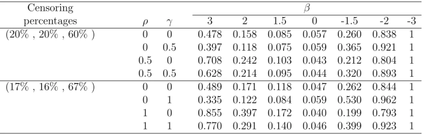
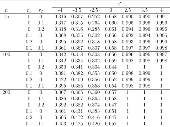
Table 2.1 presents the empirical or estimated size and power of the proposed test procedure based on the simulated data generated from the exponential distribution with

α= 2, β =−3,−2,−1.5,0, 1.5,2 or 3. Here we used theηfunction given in Section 2.3 with different values ofρandγand the self-consistency algorithm for the determination of the maximum likelihood estimates ˆFn1 and ˆFn2. In the table, the first column gives

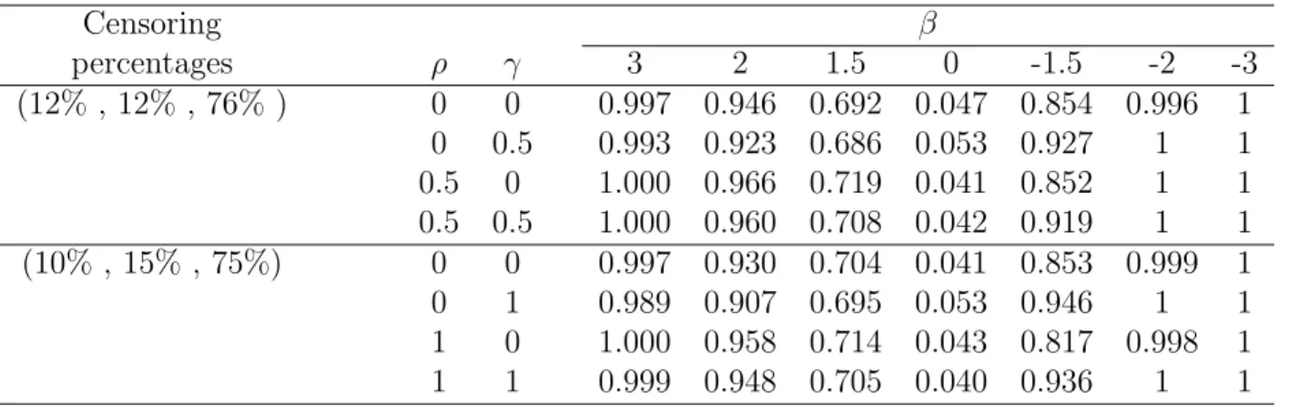
the percentages of left-censored, interval-censored and right-censored observations in the generated data, which are roughly (20%,20%,60%) and (17%,16%,67%) for the two situations considered here. The results obtained under the gamma distribution are given in Table 2.2 and here we took α= 1 and the same values for β as in Table 2.1. One can see from both Tables 2.1 and 2.2 that the proposed test procedure seems to give right size and have good power for the situations considered here.

(56)

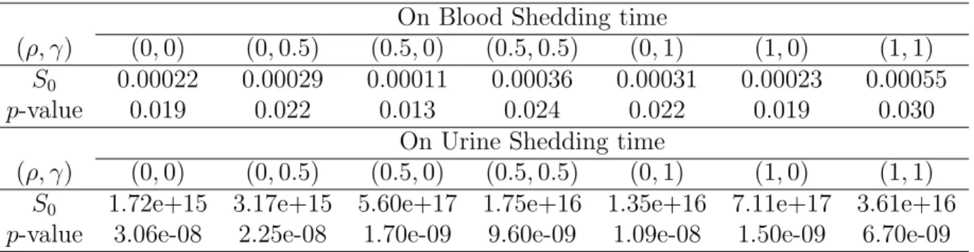
To illustrate the proposed approach, we apply it to the set of interval-censored data discussed in Goggins and Finkelstein (2000) and Sun (2006) among others. The data arose from an AIDS clinical trial concerning the opportunistic infection cytomegalovirus (CMV). During the study, among other activities, blood and urine samples were col-lected from the patients at their clinical visits and tested for the presence of CMV, which is also commonly referred to as shedding of the virus. These samples and tests provide observed information on the two variables, the times to CMV shedding in blood and urine, respectively. The study consists of 204 patients who provided at least one urine and one blood samples during the study. For some patients, their shedding had already occurred at their first clinical visits or they had not yet started shedding by the end of the study, giving either left- or right-censored observations on their shedding times. For the other patients, their shedding times were observed to belong to some intervals given by the last negative and first positive blood or urine test, respectively.

In addition to the observed information about CMV shedding times in blood and in urine, the study also provided the range of each patient’s baseline CD4 cell count. In particular, the patients were classified into two groups: these with their baseline CD4 cell counts less than 75 (cells/µl) and the others. Note that the CD4 cell count indicates the status of a person’s immune system and is commonly used to measure the stage of HIV infection. For this data set, one problem of interest is to compare the two groups of patients with respect to their CMV shedding times. For this, we applied the test procedure developed in the previous sections to the data on the times to CMV shedding in blood and urine separately and the obtained results are presented

(57)

in Table 2.3. They indicate that the CMV shedding times in both blood and urine were significantly different for the two groups of patients, especially in urine. In other words, the CMV shedding time seems to be significantly related to the baseline CD4 cell count and these results are similar to those obtained by others.

2.5 Concluding Remarks

This chapter discussed the nonparametric comparison of survival functions when only interval-censored failure time data are available. For the problem, a class of nonpara-metric tests was proposed and both finite sample and asymptotic properties of the presented approach were established. One major advantage of the proposed test pro-cedure is that its asymptotic distribution is known under both null and alternative hypotheses, which makes both power and sample size calculation possible. In contrast, for all existing nonparametric test procedures, their asymptotic distribution is either unknown or known only under the null hypothesis. Note that another shortcoming for some existing test procedures is that the estimation or determination of the variance of the test statistics involve the dealing of high dimension matrices, which makes them unstable. It is easy to see that the proposed test procedure does not have the same problem.

It should be noted that there exist some limitations about the proposed nonpara-metric test procedures. One is that in the previous sections, it was assumed that no exact observation of survival time is observed. Although this may not be true in

(58)

gen-eral, it holds in many situations such as studies with periodic follow-ups. Also one can apply the procedure if the distributions of interest have only finite support points. Of course, it would be useful to generalize the proposed approach to situations where observed data include both exact and interval-censored observations on the survival time of interest.

Another limitation of the proposed approach is that we only considered the situ-ation where the distributions generating censoring intervals are same for the subjects in different treatment groups. Sometimes this may not be true as, for example, the subjects in different treatment groups may have different follow-up patterns in a peri-odic follow-up study. One specific example of this is given by a clinical trial in which patients receiving placebo treatment may feel worse compared to other patients and thus visit doctors more often. Among others, Sun (1999) discussed this problem for current status data, a special case of interval-censored data. However, there does not seem to exist a nonparametric test procedure similar to the one proposed here for this later situation.

(59)

Chapter 3 Nonparametric Comparison of

Survival Functions Based on

Interval-Censored Data With

Unequal Censoring

3.1 Introduction

This chapter again discusses nonparametric comparison of survival functions when one observes only interval-censored failure time data. One common drawback or restriction of the nonparametric test procedures mentioned above and many given in the literature is that they can apply only to situations where the censoring variables follow the same

(60)

distribution for the subjects in different treatment groups. In other words, they require that the censoring mechanism is the same for all subjects. In practice, however, this may not be true.

In the case of current status data, for example, the single observation time on each subject may the death time and depend on the treatment. It is easy to see that in these situations, the use of the test procedures that fail to take into account this fact could result in misleading or wrong results such as seriously overestimating or underestimating the treatment difference. Among others, Sun (1999) and Zhu et al.(2008) addressed this issue and gave some nonparametric test procedures that allow the dependence of the distributions of censoring variables on treatments. However, the former is only for current status data and the latter relies on some condition that may be restrictive in practice. In the following, we present a new test procedure that applies to more general situations.

The remainder of this chapter is organized as follows. We will first introduce some notation and assumptions that will be used throughout the chapter in Section 3.2. Section 3.3 will then present the new test procedure developed by using the same idea used in Sun (1999). It can be seen as a generalization of the procedure given in Sun (1999) and includes that proposed in Zhu et al. (2008) as a special case. Also in Section 3.3, the asymptotic distribution of the test statistic is given. Section 3.4 gives some results obtained from a simulation study conducted to evaluate the performance of the proposed approach and they indicate that it works well in practice. In Section 3.5, an illustrative example is presented and Section 3.6 contains some discussion and

(61)

concluding remarks.

3.2 Notation and Assumptions

Consider a failure time study that involvesnindependent subjects andp+1 treatments. For subjecti, let Ti denote the survival time of interest and assume that the observed

information on Ti is given by

{Ui, Vi,∆1i =I(Ti ≤Ui),∆2i =I(Ui < Ti ≤Vi)},

where Ui and Vi with Ui ≤ Vi are two random variables representing two observation

times on the subject, i = 1, . . . , n. That is, we have interval-censored data on theTi’s.

It is easy to see that ∆1i = 1 means that the observation on Ti is left censored, while

∆3i = 1−∆1i−∆2i = 1 corresponds to a right-censored observation onTi. DefineZi

to be the p dimensional treatment indicator vector whose l element being equal to 1 if subject i is given treatmentl and 0 otherwise, l = 1, ..., p, and let Sj(t) denote the

survival function of the subjects given treatmentj,j = 1, ..., p+ 1. Then the observed data are {Ui, Vi,∆1i,∆2i, Zi;i= 1, ..., n}. Our goal is test the hypothesis

H0 : S1(t) = ... = Sp+1(t).

(62)

on the treatment indicator Zi, but they are independent of the survival time Ti given

Zi. To model the dependence, following Wang et al. (2010), we will assume that the

hazard functions of Ui and Vi have the form

λU_i (t|Zi) = λ1(t) exp(γ10Zi) (1)

and

λV_i (t|Zi) = I(t > Ui)λ2(t) exp(γ20Zi), (2)

respectively. In the above, λ1(t) and λ2(t) denote some unknown baseline hazard

functions and γ1 and γ2 are vectors of regression parameters. Under models (1) and

(2), the baseline survival functions of Ui and Vi have the forms

S1(t) = exp − Z t 0 λ1(s)ds =: exp{ −Λ1(t)}, and S2(t) = exp − Z t 0 I(s > Ui)λ2(s)ds =: exp{ −Λ2(t)} , respectively.

Before ending this section and presenting the proposed test statistic in the next section, we will briefly review the test statistic developed by Sun (1999) for current status data. For this, define Ni(t) = I(t ≥ Ti), ˜N1i(t) = I(t ≥ Ui), and ˜N2i(t) =

The nonparametric analysis of interval-censored failure time data