Trap Coverage: Allowing Coverage Holes of
Bounded Diameter in Wireless Sensor Networks
Paul Balister
§Zizhan Zheng
†Santosh Kumar
§Prasun Sinha
†§University of Memphis †The Ohio State University {pbalistr,santosh.kumar}@memphis.edu {zhengz,prasun}@cse.ohio-state.edu Abstract—Tracking of movements such as that of people,
animals, vehicles, or of phenomena such as fire, can be achieved by deploying a wireless sensor network. So far only prototype systems have been deployed and hence the issue of scale has not become critical. Real-life deployments, however, will be at large scale and achieving this scale will become prohibitively expensive if we require every point in the region to be covered (i.e., full coverage), as has been the case in prototype deployments.
In this paper we therefore propose a new model of coverage, called Trap Coverage, that scales well with large deployment regions. A sensor network providing Trap Coverageguarantees that any moving object or phenomena can move at most a (known) displacement before it is guaranteed to be detected by the network, for any trajectory and speed. Applications aside, trap coverage generalizes the de-facto model of full coverage by allowing holes of a given maximum diameter. From a prob-abilistic analysis perspective, the trap coverage model explains the continuum between percolation (when coverage holes become finite) and full coverage (when coverage holes cease to exist).
We take first steps toward establishing a strong foundation for this new model of coverage. We derive reliable, explicit estimates for the density needed to achieve trap coverage with a given diameter when sensors are deployed randomly. Our density estimates are more accurate than those obtained using asymptotic critical conditions. We show by simulation that our analytical predictions of density are quite accurate even for small networks. We then propose polynomial-time algorithms to determine the level of trap coverage achieved once sensors are deployed on the ground. Finally, we point out several new research problems that arise by the introduction of the trap coverage model.
I. INTRODUCTION
Several promising applications of wireless sensor networks with a high potential to impact human society involve de-tection and tracking of movements. Movements may be of persons, animals, and vehicles, or of phenomena such as fire. Examples include tracking of thieves fleeing with stolen objects in a city, tracking of intruders crossing a secure perime-ter, tracking of enemy movements in a battlefield, tracking of animals in forests, tracking the spread of forest fire, and monitoring the spread of crop disease.
So far only prototype systems have been deployed and hence the issue of scale has not become critical. Real-life deployments, however, will be at large scale, and achieving this scale will become prohibitively expensive if we require every point in the region to be covered (i.e., full coverage or blanket coverage [18]), as has been the case in prototype deployments [13], [16], [21]. The requirement of full coverage will soon become a bottleneck as we begin to see real-life deployments.
In this paper, we therefore propose a new model of coverage, calledTrap Coverage, that scales well with large deployment regions. We define a Coverage Hole in a target region of deployment A to be a connected component1 of the set of uncovered points of A. A sensor network is said to provide
Trap Coveragewith diameter d toAif the diameter of any Coverage Hole inA is at mostd.For every deployment that provides trap coverage with diameter ofd, the sensor network guarantees that every moving object or phenomena of interest will surely be detected for every displacementdthat it travels inA. At any instant, we can either pin point the location of a moving object precisely, or can point to a coverage hole of diameter at mostdin which it istrapped.
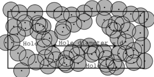
With this model, the density of sensors can be adjusted to meet the desired quality of tracking while economizing on the number of sensors needed. Large scale sensor deployments for tracking thus become economically feasible with this new model of coverage. Figure 1 shows an example deployment region where the size of the largest uncovered region isd.
Hole diameter = d Hole
Hole
Fig. 1. In this deployment, d is the diameter of the largest hole. Notice that although the diameter line intersects a covered section, it still represents the largest displacement that a moving object can travel within the target region without being detected.
Trap Coverage Generalizes Full Coverage: If the value of
dis set to 0, then trap coverage is equivalent to full coverage. By relaxing the requirement of having every point covered, trap coverage generalizes the model of full coverage.
Traditionally, the fraction of target region that is covered has been used as an indicator of the quality of coverage [13], [25]. Notice that even if a large fraction of region is covered, the diameter of the largest hole may be arbitrarily large. Therefore, trap coverage may better indicate theQuality of Full Coverage as it provides a deterministic guarantee in the worst case.
1Here connectedrefers to the connectivity of a set of points in the real plane that comprise the target region.
II. KEYCONTRIBUTIONS ANDROADMAP
In addition to introducing a new model that generalizes the traditionalfull coveragemodel, we make several contributions in this paper, some of which may be of independent interest.
First, we derive a reliable estimate of the density (similar as in [3]) needed to achieve trap coverage with a desired diameter
dwhen sensors are deployed randomly. Roughly speaking, the critical density condition is of the form
λ(2rd+πr2)≈logn, (1) where λis the expected density of sensors per unit area, ris the sensing range, and n=λ|A|is the expected total number of sensors in the target region A. In other words, we expect that having, on average, lognsensors in the r neighborhood of a thin long hole of diameter d will suffice for achieving trap coverage with a diameter of d. We also show how our estimate for the density can be adapted to a non-disk model of sensing region, by using ellipses of random orientation as an example. (Section IV)
Second, the model of trap coverage explains the gap that has long existed between the percolation threshold (when holes become finite and isolated) and the critical density for achieving full coverage (when holes cease to exist). Looking at (1), we can observe that if r is constant w.r.t. n, which is the case for percolation to occur, d is of the order of logn, matching the known behavior that for fixed λr2 above the percolation threshold, the maximum hole diameter is on average of order logn. On the other hand, if dis a constant, and 0 in particular, then λr2 is of the order of π1logn, matching the known behavior for achieving full coverage [18]. Thus, the trap coverage model not only generalizes the model of full coverage, it also helps explain the probabilistic behavior of coverage between the percolation threshold and critical density for full coverage. (See Figure 6 for an illustration.)
Once sensors have been deployed on the ground (either randomly or deterministically), it may be necessary to de-termine the level of trap coverage that they provide, since some may fail at or after the deployment for unforeseen reasons. Ourthirdcontribution, therefore, is polynomial time algorithms to determine the level of trap coverage that an arbitrary deployed sensor network provides. Our algorithms not only works for non-convex models of sensing regions, but also when sensing regions are uncertain (e.g., probabilistic sensing models). Further, they take into consideration the complications that may arise due to the boundary of the deployment region (see Figure 8 for an example). (Section V)
III. RELATEDWORK
Most work on probabilistic density estimates for coverage assume the full coverage model [18], [24], [30]. As we show in Section IV, the na¨ıve approach of increasing the sensing range by dand then deriving the conditions for full coverage will lead to overdeployment, no matter how small the value of d > 0 is. For larger d, overdeployment will be orders of magnitude more than needed in our estimates.
Work on full coverage that does consider holes focuses on the fraction of region that is (un)covered, see [24], [30]. They attempt to asymptotically minimize the area of vacant region and do not provide any simple expression for the density needed in a random deployment to achieve a desired fraction of uncovered region. Even if there existed such an expression, it could not be used to readily derive an estimate of density needed for bounding the diameter of coverage holes. This is because holes of large diameter tend to be long and thin, and their area is not typically large (even close to zero).
Perhaps, the work closest to trap coverage are [8], [11] that allow holes for surveillance applications. Here the quality of surveillance metric is based on the distance that a moving target, starting at a random location, moving in a random direction can travel in astraight line before it is detected by a sensor. In [8], distance to detection by a giant connected component is also studied. There are several issues with such a metric. For one, they do not provide any worst case guarantee on how far a target can move before being detected, unlike trap coverage. For example, if the density chosen is just large enough that a giant component exists almost surely, as in [8], the hole diameters are not bounded by any constant; they grow as a function oflognwherenis the number of sensors deployed. Further, even though the average distance may be bounded, even close to zero, the worst case distance could be arbitrarily large (as show in Figure 2). As shown in a typical deployment (Figure 4), holes that have larger diameters are usually thin and long, so the average distance measure is quite likely to be misleading. Therefore, neither of these metric can be used to derive a density estimate for trap coverage.
In summary, there does not exist any work that can be used to derive estimates of density (or even critical conditions) needed in a random deployment to achieve trap coverage of a given diameter, a mathematically challenging problem that we address comprehensively in this paper. We postpone discussing existing work related to algorithmic determination of the status of trap coverage to Section V-A.
IV. ESTIMATING THEDENSITY FORRANDOM DEPLOYMENTS
In this section, we derive a reliable estimate for density that will ensure trap coverage of a given diameter. We take a progressive approach in deriving our estimate for simplicity of exposition. We first consider a disk model of sensing. For this model, we first derive a crude but rigorous bound that may appeal to intuition. We then show that large holes occur with a Poisson distribution. In Section IV-A, we estimate the intensity of this Poisson distribution. Once we have an accurate estimate of the intensity with which large holes occur, we can accurately determine the density needed to achieve trap coverage of a given diameter d with any given probability (such as with probability 0.9999). We show in Section IV-B that our density estimate is accurate even for small deployment regions, a significant improvement over asymptotic critical densities that work only for large deployments. Finally, we show in Section IV-C, how our derivations can be adapted
R
L
Fig. 2. RegionRand lineLin proof of lower bound onP(hm≥d). Lis uncovered and so forms a long thin hole providedRis void of any sensors.
to non-disk sensing models. We provide the derivation for randomly oriented ellipses as an example.
We consider a Poisson deployment with intensity λ in a deployment region A that includes a large target region A of area |A|. Write n = λ|A| for the expected number of sensors within the target region, and hm for the maximum hole diameter.
Before we obtain a bound on the probability that hm≥d, we make some remarks on the effect of the boundary. Gen-erally speaking, if the deployment region A is the same as the target region A, then coverage is more likely to fail at the boundary than in the interior (see [3]). Thus a similar result would be expected to occur for trap coverage, at least when d/r is small. One simple way of avoiding problems at the boundary is to enlarge A so that it includes all points within distance r of A. (We shall assume in the following that the boundary ofAis small, i.e.,|∂A|(r+d) |A|. Thus enlarging the deployment region as above will not increase its area much, i.e.,|A|/|A| ≈1.) This makes coverage of points on the boundary of A as likely as points in the interior, and large holes are no more likely to appear at the boundary than in the interior (in fact less likely since there is less area near the boundary than the interior, and holes are confined to lie insideA). In the following analysis we shall assume that the deployment region has been enlarged in this manner.
We first derive a lower bound on P(hm ≥d). Let Lbe a straight line of lengthdinsideA. If there is no sensor within distance r of L then L lies in the interior of a hole, which then must have diameter at leastd. LetR be the set of points within distancerof L. ThenRconsists of a2r×drectangle with two semicircular caps of radius r attached to each end (see Figure 2). The probability that R contains no sensor is
e−λ|R| where |R| = 2rd+πr2. We can place R inside a 2r×(d+ 2r)rectangle which has area less than 2|R|. Thus if Ais large enough and of a reasonable shape (in particular, if it has small boundary as mentioned above), we can pack at least|A|/(2|R|) =n/(2λ|R|)disjoint copies ofRintoA. The event that one copy ofRis devoid of sensors is independent of any of the other copies, so the probability that the maximum hole diameter is at leastdis bounded below by the probability that at least one of the copies of Ris empty. Thus
P(hm≥d)≥1−
1−e−λ|R|n/(2λ|R|)≥1−e−I|A|,
where I= (2(2rd+πr2))−1e−λ(2rd+πr2). (2) (Here we have used the fact that 1−x≤e−x. The quantity
I is essentially a bound on the average number of holes of diameter ≥dper unit area.) If we write
λ(2rd+πr2) =λ|R|= logn−log logn−t, (3)
dq
p q
p q
γ
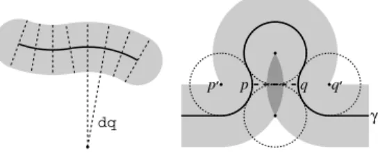
Fig. 3. Left: calculation of the area of Rγ(s). Right: Example of
self-overlappingRγ(s)withs=r.R1 is lightly shaded region,R2 is heavily shaded region. Ifγ approaches within2(√3−1)r > rof itself, then one can shortenγby cutting across along dashed linepq.
then for t = t(n) = o(logn), I|A| = 2(logne−tlog loglogn n−t) = (.5 +o(1))et. If t→ ∞ as n→ ∞ we haveI|A| → ∞ and thusP(hm≥d)→1.
Now, we give an upper bound on P(hm ≥ d), which is more involved. Suppose a holeH of diameterhm≥dexists. Supposex, y∈Hare points with x−y =dand letγbe the shortest path fromxtoy inside the holeH. We may assume thatxlies at a crossing point of the boundaries of the sensing regions of two sensors (see Lemma 5.1 below). Note that γ
consists of straight line segments possibly joined together with arcs of circles of radiusr. In particular, the radius of curvature of γat any point is never less than r.
Lemma 4.1: Suppose 0 < s ≤ r. Then the set Rγ(s) of points that lie within distancesof γhas area at leasts(|γ|+
d) +πs2, where|γ| ≥dis the arc length of the curveγ. Proof: Suppose first that Rγ(s) does not wrap around on itself, i.e., no point on ∂Rγ(s) is distance s from more than one point of γ (see Figure 3). Then the area of Rγ(s) is exactly2s|γ|+πs2. To see this, cutγinto small segments each of (approximately) constant radius of curvature, and make corresponding cuts in Rγ(s) orthogonally to γ at the places where γ is cut. Suppose one segment of γ has radius of curvature R and subtends an angle δθ. The length of this segment isRδθ, while the area of the corresponding slice of
Rγ(s)is 12(R+s)2δθ−12(R−s)2δθ= 2sRδθ(the difference
between sectors of two disks). Adding up these areas for each segment ofγgives an area of2s|γ|, and adding the two half-disks centered at the endpoints ofγ gives the result.
Now assumeRγ(s)self-intersects. Then the above argument will overestimate the area. However, distant parts ofγ cannot approach too closely. Indeed, suppose there are two points
p and q on γ such that p = q and the distance between p
and q is a local minimum for points on γ. Then there are sensors at p, q with p, q lying on the segment pq and γ
following the boundaries of the sensor regions of p and q
(see Figure 3). No sensor on the opposite side of γtop and
q can have a sensor region intersecting the sensor regions of
p orq, but if p−q <2√3rthis implies no sensor region intersects the line segmentpq. Thus if p−q <2(√3−1)r
the line segment fromptoqis uncovered by any sensor andγ
can be shortened by joining across fromptoq, contradicting the assumption that γ was the shortest path from x to y. A similar argument shows that no point can lie in a triple
self-intersection of Rγ(s). Indeed, if w is such a point and p1,
p2,p3 are distinct locally closest points on γ, then there are sensors atpi, wherepilies on the segmentwpiandγ follows the boundary of the sensor region ofpi nearpi. If any of the distances pi−pj , i= j, are less than 2
√
3r, then γ may be shortened. But if all pi−pj ≥ 2
√
3r then their sensor regions do not intersect, and so wdoes not exist.
Thus of the area|Rγ(s)|, no part can be more than double counted by the estimate2s|γ|+πs2above. In other words, we can writeRγ(s)as the union of two regionsR1 andR2, with |R1|+ 2|R2| = 2s|γ|+πs2. Now any line L perpendicular to xy between x and y must intersect R1 in line segments of total length at least 2s since no point on L before the first point of γ or after the last point of γ can be in a self-intersection of Rγ(s). Also R1 contains two half-disks atx andy. Thus |R1| ≥2sd+πs2 and|Rγ(s)|=|R1|+|R2|= |R1|/2 + (|R1|+ 2|R2|)/2≥s(|γ|+d) +πs2 as required.
Now approximateγ with a path γ that is made up from a sequence of arcs of circles, each of radius r/2and length rε
(so they curve by an angle of 2ε). Each arc curves either to the left or the right. One can show that γ can be chosen so that it starts atx, the angle thatγ makes with the horizontal atxis a multiple ofε, and all points ofγare within distance
Crε2 of γ, where C is some absolute constant. Hence there is no sensor within distance r(1−Cε2)of γ.
Givenx, there are(2π/ε)2kchoices forγwhenγ consists ofksegments. Givenγ, one knowsγto within distanceCrε2, so picking anyγconsistent withγ, we knowRγ(r(1−2Cε2)) contains no sensors. Since the length of γ and γ agree to within a factor of 1 +O(ε2), any γ gives us a region of area (r2kε+rd+πr2)(1−Cε2) devoid of sensors, so the probability of some suchγ existing starting fromxis at most
k≥d/rε(2π/ε)2ke−λ(r 2kε+rd+πr2)(1−Cε2) ≤ 2π ε(1−2e−λr2ε/2)e−λ (2rd+πr2)(1−Cε2)+(d/rε) log 2
Setting ε= (λr2)−2/3 and assumingλr21, this is at most
C(λr2)2/3e−λ(2rd+πr2)(1−O((λr2)−2/3). (4) The expected number of intersection points in A we can choose for xis4λπr2n, so we obtain
P(hm≥d)≤C(λr2)5/3ne−λ(2rd+πr
2)(1−O((λr2)−2/3) (5) for some constant C. For λr2 =O(logn), this tends to 0 when
λ(2rd+πr2)(1−O((λr2)−2/3))≥logn+O(log logn).
Combining this with the lower bound (3) above, we see that the maximum hole sizehm=dtypically occurs when
λ(2rd+πr2)(1−O((λr2)−2/3)) = logn, (6) (the O((λr2)−2/3) error term swallowing thelog logn terms in both cases). We observe that (from both the lower and upper bounds above) the holes with the largest diameter are long and thin, basically being obtained by insisting that
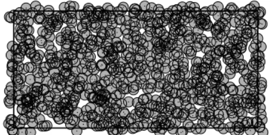
Fig. 4. Example of Poisson deployment. Rectangle denotes target region. Notice that holes of larger diameters are typically long and thin, although this need not be true for smaller diameter holes.
an almost straight path γ of length d is not covered by any sensing region. We show in Figure 4, a representative Poisson deployment for which some holes exist. Note that although the holes are of various shapes, the holes with the largest diameters are usually “long and thin”, confirming our analytical conclusion.
Comparison with an obvious extension of the full coverage model.Note that our estimate is significantly better than the na¨ıve bound obtained by increasingrbydand then demanding that this provides full coverage. Indeed, our bound (assuming
λr21) is of the form
λ(2rd+πr2)≈logn, (7) while if we required full coverage with sensing range r+d
we would need (replacingdby 0 and rby r+din (7))
λπ(r+d)2=λ(πd2+ 2πrd+πr2)≈logn.
Even for smalld we would underestimatedby a factor ofπ
(2πrd vs. 2rd), and for large d the discrepancy tends to ∞ (d ∼ c√logn vs. d ∼ cr−1logn for fixed λ). Note that enlarging the sensor range byd/2is not sufficient in general to eliminate all holes of diameter d, but even if it were, the (incorrect) bound obtained on dwould still always be worse than our result. The reason for the discrepancy between our estimate and the na¨ıve bound however becomes clear when we observe that a long thin hole can be covered with just a small increase in r, rather than increasing it byd.
Estimating the Probability Distribution of Large Holes.
Large holes, when they exist, should be well separated, so one would expect the distribution of the number of holes with diameter≥dto follow an approximately Poisson distribution. This is indeed true for largeλr2. To show this, supposeH is a coverage hole. ThenH depends on the Poisson process within a regionHconsisting of all points at distance≤rfromH. To show the number of holes is approximately Poisson, one can use the Stein-Chen method (see [1]). In our case, it reduces to showing (a) that the expected number of pairs of holes
H1 and H2 for which H1 andH2 intersect is o(1), and (b)
that this would also be true if theHi were truly independent. Condition (b) is easy to show since the Hi are much smaller thanA. Condition (a) holds since conditioned of the state of the Poisson process inH1, it is unlikely there is a hole close
the boundary of a deployment region R2\H1, which holds
since the boundary ofH1 is typically not large.) We refer the
reader to [4] for more details of these calculations. As a result, for sufficiently large λπr2
P(hm≥d)≈1−e−I|A|, where (8)
I=λe−λ(2rd+πr2)(1−O((λr2)−2/3),
I being the expected number of holes of diameter at least d
per unit area (i.e., the intensity of the Poisson process for the occurrence of holes of diameter ≥ d). Once again the O() error term in I swallows the polynomial factors in front of the exponentials in the upper and lower bounds given above. We shall refine this estimate in the next section.
A. Refining the Estimate
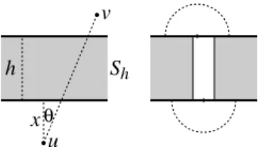
In this section we shall give a much more accurate estimate for the probability of occurrence of holes of diameter ≥ d. We only provide an outline of our derivation here and defer the detailed proofs to [4]. To obtain an improved estimate, we compare the trap coverage model with that of barrier coverage, where sensors are deployed in a long (but 2 di-mensional) horizontal rectangular strip Sh of height h, and one asks whether there are coverage holes crossing the strip (see [3] for details). We shall count the number of holes that cut across this strip in two different ways, leading to a comparison between barrier coverage and trap coverage. First letIdtrap be the number of holes of diameter at leastdper unit area and assumeu, vare endpoints of such a hole withulying belowv. Then since the holes are typically long and thin, this hole will cut acrossShprovideduandvlie on opposite sides ofSh. Letθbe the angleuvmakes with the vertical, andxthe distance ofubelow the bottom ofSh(see Figure 5). Then we need u−v ≥(x+h)/cosθ. The intensityIof such holes per unit length alongSh is therefore given approximately by
I≈ 1 π π/2 −π/2 ∞ 0 I trap (x+h)/cosθdxdθ.
To relate this toIdtrapat a particular value ofd, we note that by our simple estimates in the previous section that Idtrap decays exponentially with d,
Idtrap+ε≈I
trap
d e−
2λrε.
Using this approximation (and evaluating thex-integral) gives
I≈Ihtrap 1 2πλr π/2 −π/2e −2λrh(1/cosθ−1)cosθ dθ ≈Ihtrap(4πλ2r2(λrh+98))−1/2,
where the last approximation is valid for largeλrh.
Now we evaluateIby comparison with barrier coverage. A hole across Sh results in a break as defined in [3], however when defining barrier coverage one assumes deployment only insidethe stripSh. Thus for a break to define a hole crossing
Sh, we also need that sensors outside of Sh do not destroy the break. From the results in [3] we know that most breaks are approximately rectangular and thin cutting perpendicularly
Sh x u v h θ
Fig. 5. Left: hole with diameter uv crossing strip Sh. Right: additional vacant semicircular areas allow break to form hole.
across Sh. Using this it follows that for this break to make a hole, one needs at least one point on the top boundary of Sh inside the break to be uncovered by sensors outside of Sh, and similarly at least one point on the bottom boundary of
Sh to be uncovered (see Figure 5). One can show that the probability of some point on the top boundary of Sh in a fixed interval of lengthW to be uncovered by sensors above
Sh is approximately (1 +λrW)e−πλr 2/2
. One may assume the top and bottom boundaries are independent for largeh(in factλh3ris enough), so this gives
I≈Ihbarrier(1 +λrE(W))
2
e−πλr2,
where E(W)is the expected width of the uncovered interval on the boundary ofShthat occurs at a break, andIhbarrieris the average number of breaks per unit distance alongSh. One can show using the techniques of [3] thatE(W)∼cλ−2/3r−1/3
withc≈0.72. Also [3] gives the following estimate forIhbarrier.
Ihbarrier≈λ2/3(2r)1/3e−2λrd(1−α(4λr
2)−2/3)+β
.
where α≈1.12794 andβ ≈ −1.05116. (Note that the value of r in [3] is twicethe sensor radius.) Putting these together gives the following approximation for Idtrap.
Idtrap≈C0λ(λr2)2/3(1 +c(λr2)1/3)2(λrd+98)1/2
×e−2λrd(1−α(4λr2)−2/3)−πλr2, (9) where C0=π1/224/3eβ ≈1.5611, α≈1.12794, c≈0.72.
As in [3], this estimate should be valid for λd3 r, and
λr21, which in our context means not too close to either full coverageπλr2∼lognor the percolation thresholdλr2∼
constant.
Since coverage holes of diameter ≥ d follow Poisson distribution (using the same Stein-Chen argument as in the previous section), we have
P(hm≥d)≈1−e−|A|I
trap
d (10)
when Idtrap is small.
B. Simulation to Validate Our Density Estimates
In this section, we present some simulation results to sup-port our analytical results. We consider a deployment region A of size 256r×256r, where we place points according to Poisson process of intensityN. We varyN from0to500,000 and track the maximum coverage hole diameter. We repeat our experiment 10,000 times for each value ofN for statistical accuracy. We also ran simulations with smaller A, obtaining very similar results even down to a 8r×8r region. We have two distinct goals in our simulation.
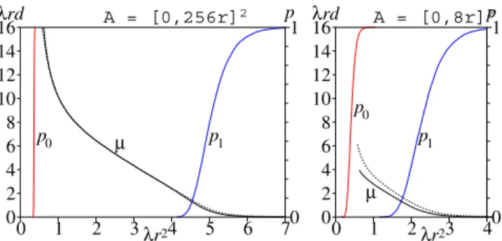
0 1 2 3 4 5 6 70 1 λr2 0 2 4 6 8 10 12 14 16 p0 μ p1 0 1 2 3 40 1 λr2 0 2 4 6 8 10 12 14 16 p0 p1 μ
Fig. 6. Mean size of largest hole (μ, left hand scale) together with estimate based on (9) and (10) (dotted line). Probability (right hand scale) that hole size becomes finite (p0), i.e., percolation occurs, and probability that holes cease to exist (p1), i.e., full coverage occurs.
1.) Validating the accuracy of our analytical estimates.
We show results of our simulation in Figures 6 and 7. We first explain our rationale for picking the various axis before explaining the results. For x-axis in Figure 6, we useλr2, a dimensionless parameter which indicates the level of coverage. (Each point is covered by an average ofπλr2sensing regions.) We have two parameters for the y-axis. On the left scale, we use λrd, a dimensionless quantity to measure the hole diameter, which also happens to be the x-axis in Figure 7. Since d decreases with an increase inλ or r, using this unit allows us to present the entire spectrum of variation in the hole diameter in one graph. The right scale of y-axis in Figures 6 and the left scale in Figure 7 are probabilities. Note that the only quantity fixed in Figure 6 is the size of Arelative tor. We observe that the mean value of the maximum hole diameter observed in simulation (solid line) is mostly indis-tinguishable from our analytical estimates (dotted line) for 256r×256rregion and quite close even for the8r×8rregion, which is smaller than many real-life deployments.
In Figure 7, we show the entire probability distribution for hole diameters for some densities, which provides significantly more information than the mean values of diameter. This con-firms that our estimate of the probability distribution of hole diameters (to Poisson) and our estimation of the parameter of this distribution are highly accurate, making it quite useful in real-life deployments.
2.) Graphically demonstrating the new continuum from percolation to full coverage.
Figure 6 illustrates how the model of trap coverage fills the continuum between percolation and full coverage. The curve labeled p0 depicts the probability of percolation, i.e., largest hole diameters becoming smaller than the deployment region. As the density increases, hole diameter decreases. The curve labeled p1 depicts the probability of full coverage. As
this curve approaches 1, the expected largest hole diameter approaches zero. Note that the value ofλr2 corresponding to
p0 represents percolation threshold, while that corresponding
top1represents critical conditions for full coverage. Until this
result of ours, the behavior in between these two important values of λr2 was unknown. The introduction of the trap coverage model in this paper now explains the continuum
0 1 2 3 4 5 6 7 8 9 10 0 1 λrd p 1 2 3 4 5 6
Fig. 7. Cumulative probability distribution, P(hm ≥d), of largest
hole size for λr2 = 1, . . . ,6, together with estimate based on equation (9) and (10) (dotted line). For example, ifλ= 1, andr= 2 (so λr2 = 4), then from Figure 6, left side, we have λrd≈ 2on average (so d ≈ 1), however it can range between about 1 and 6 (d= 0.5to 3) with a probability distribution as shown here.
between these two important curves comprehensively, with the curve for the trap coverage diameter.
C. Extending to Non-disk Sensing Regions
The above analysis assumes that the sensing regions are disks. However, it is clear from the lower bound argument for P(hm ≥ d) that we can generalize this to other shapes of sensing region. To recall, for the lower bound we require that no sensing region intersects a lineL. The probability that this occurs can be calculated for any required (even probabilistic) model of the sensing region. The fact that the upper bound for disks is close to the lower bound suggests that this will also hold for most reasonably “disk-like” sensing regions. As an example, we consider the case of randomly oriented ellipses (to model biased gain along a randomly oriented axis).
Lemma 4.2: Suppose the sensing regions are ellipses, each with maximum and minimum radiirandαrrespectively, and with orientation that is random and uniform. Then the expected number of sensor regions meeting a fixed line L of length d
is given exactly by
λ(πr2α+ 2rdπ2E(1−α2)), (11) where E(m) =0π/2(1−msin2θ)1/2 is an elliptic integral.
Proof:Consider the sensors whose smaller radius lies in some small angle[θ, θ+dθ]from the direction of the lineL. These sensors occur as a Poisson process of intensity 2λπdθ. If we scale the plane by stretching by a factor 1/α in the direction of the smaller radius, the sensor regions become circular with radius r, while the density of sensors is now
αλ
2πdθ. The lineLis now also stretched, and has a new length
d=d(α−2cos2θ+ sin2θ)1/2. The expected number of these sensors meeting Lis therefore equal to
(πr2+ 2rd)α2λπdθ
= 2λπ(πr2α+ 2rd(1−(1−α2) sin2θ)1/2)dθ.
The result follows by integrating this from θ= 0 to2π. Note that since we are assuming Poisson deployment, the physical location of the sensor within the ellipse is irrelevant (as long as it is independent of the location and orientation
of the ellipse), so we may for example assume the sensor is at the center, or at a focal point, or at one end of the ellipse. The results will be identical in all cases. The lower bound argument forP(hm≥d)follows exactly as before, using (11) in place of the expression λ|R| = λ(πr2+ 2rd). Similarly, the upper bound argument also follows, except that the radii of curvature of the pathγmay need to be reduced, leading to worse constants in theO()term in (5) whenαis small.
Similar results can be shown for probabilistic sensing re-gions. For example, if the radii r varied randomly then one obtains the same results with λ|R| replaced with Eλ|R| =
λ(πE(r2)+2E(r)d)(for the disk model), provided the random radii ris is bounded, r1 < r < r2, and with the error terms depending on r1 andr2.
V. COMPUTING THETRAPCOVERAGEDIAMETER Even though we provide an accurate probabilistic estimate of the density needed to achieve trap coverage of a given diameter when deploying sensors randomly, it may be useful to ascertain deterministically whether a target hole diameter has been achieved after deployment, especially in the face of unanticipated and unknown deployment failures [5]. In order to determine whether a deployed network continues to provide trap coverage over time, efficient algorithms are needed to determine the largest hole diameter. In this section, we propose such algorithms.
Figure 8 shows a target region with several sensing coverage holes. Although the sensors are plotted as disks in the figure, we are not assuming a disk sensing model. Further, the sensing regions of different sensors may be different. Except in Section V-D, where sensing regions are assumed to be star convex, the only assumptions we make are: 1) Two sensor nodes are within the transmission range of each other if their sensing regions overlap; 2) The accurate positions of nodes can be determined; 3) The boundary ∂Aof the target region A is a simple polygon and is known.
To determine the largest diameter of coverage holes, the following two steps are applied. First, the boundary of each hole is found. Second, the diameters of these holes are com-puted based on their boundaries to obtain the largest diameter. The good news is that several ideas from existing work on discovering exact hole boundaries [6], [14], [22], [25], [28] can be applied here. However, the following challenges, which are critical to the trap coverage model, are not addressed there. 1) The boundary of a coverage hole may involve part of
∂A, such as hole H7 in Figure 8, so that it is hard to
discover the entire boundary.
2) In a realistic sensing model, the boundary of a coverage hole may have an arbitrary shape, which makes the computation of the accurate diameter non-trivial. 3) When the shapes of sensing regions are unknown
or uncertain (as in probabilistic sensing models), the boundaries of individual holes may not be accurately determined.
We describe in Sections V-B and V-C a modification to existing algorithms that computes an accurate diameter for
H1 H2 H3 H4 H5 H6 H7 H8
Fig. 8. An instance of deployment with eight coverage holes, H1 toH8. The rectangle shows the boundary of the target region. Note that only the holes within the target region are counted. The small disks are sensing regions.
convex sensing regions and approximate diameter for non-convex but known sensing regions. In Section V-D, we de-scribe an outline of a simpler algorithm that computes an ap-proximate diameter for both known and unknown (uncertain) sensing regions. We first review existing work in this area before describing our algorithms.
A. Related Work
Tools from both algebraic topology and computational ge-ometry have been used for detecting coverage holes. Most focus on coverage verification and boundary node detection without computing the exact hole boundaries [6], [10], [14], [23], [25], [28], and several of them assume a disk sensing model and an open target region [6], [10], [23], [25], [28].
In topology based approaches, certain criteria to detect holes or verify coverage [10], [23] are derived from the topology of the covered region without using the positions of nodes. However, these criteria are computed in a centralized way and the complexity is not well studied yet. In contrast, geometry based approaches assume the positions of nodes are known [14], [25], [28] or at least the accurate distances among neighboring nodes are known [6] and use certain locally computable geometric objects to detect nodes on a coverage boundary. The first localized approach is proposed in [14] where every node can locally determine whether it is on the boundary of ak-coverage hole by counting the coverage levels of its sensing perimeter, which is simplified in the case of 1-coverage in [29]. The location free version of [14] is proposed in [6]. Another geometric approach uses Voronoi diagrams [9], [25], [28], which is not applicable to non-convex or heterogeneous sensing regions.
Based on [14], [22] proposes an algorithm to determine exact boundaries of coverage holes. However, it can only find those boundaries with at most one piece from∂A, such asH5
andH6 in Figure 8, and it assumes a disk sensing model. An
algorithm to find the boundaries of routing holes is proposed in [9], and [27] proposes a method to determine the boundaries of communication holes using only the connectivity graph and a general sensing model. However, ∂A is not considered in either approach.
B. Discovering Hole Boundary
In this and the next section, we assume that each node knows the shape of its sensing region (not necessarily convex). The impact of sensing uncertainty is discussed in Section V-D.
Our algorithm first applies the perimeter coverage based approach [14] to detect nodes on the boundaries of coverage holes. The idea is that the sensing perimeter of one node is divided into one or more pieces by the sensing perimeters of the neighboring nodes. Every such piece is called a sensing segment. A node is on the boundary of a coverage hole iff it has a sensing segment that is not covered by other nodes.
The boundaries of coverage holes needed for diameter com-putation are then derived based on the following observations, which can be verified in Figure 8. First, the boundary of a coverage hole is composed of one or more closed curves, but its diameter is only determined by the outermost one, called the hole loop. For instance,H3in Figure 8 has two boundary
curves, but the inner one – the perimeter of the two overlapped sensing regions – can be safely ignored. Second, if a hole is completely contained in another hole, it can be ignored, such as H8 in Figure 8. Third, each curve is composed of sensing segments and (possibly) parts of∂A. If it is composed of only sensing segments, the entire curve can be found by traversing the nodes on it. Otherwise, each piece that is composed of only sensing segments on the curve can be found. Once all the pieces of hole boundaries are known, a polygon clipper algorithm [20] can be extended to find the hole loops by also taking ∂Ainto account. We defer the details to [4].
C. Diameter Computation
LetH denote a hole loop, andXH denote the set of cross-ings on that loop, where a crossing is defined as an intersection point of either two sensing perimeters, or a sensing perimeter with∂A, or a vertex of the simple polygon∂A. The following lemma states thatXH is indeed a good approximation ofHin terms of the diameters, even if sensing region is not convex.
Lemma 5.1: diamXH≤diamH ≤diamXH+2D, where
D is the maximum diameter of all sensing regions. Moreover, if the sensing regions are convex, then diamXH = diamH.
Proof: diamXH≤diamH follows sinceXH ⊆H. Let
xandy be two points onH with x−y = diamH, where · denotes the Euclidean distance. Let x be the crossing on H closest to x, and y the crossing closest to y. Then
x−y ≤ x−y + x−x + y−y ≤ x−y +2D. As
x−y ≤diamXH,diamH = x−y ≤diamXH+ 2D. If the sensing regions are convex, thenHis contained within the convex hull of XH. Since a point set and its convex hull have the same diameter, the result follows.
According to Lemma 5.1, when the sensing regions are all convex, it suffices to maintain the set of crossings on each hole loop instead of their accurate shapes in order to find the largest diameter D. For arbitrary sensing regions, this also gives a good approximation when D2D.
D. Coping with Sensing Region Uncertainty
Sensing regions show irregularity due to hardware cali-bration and obstacles and therefore are hard to characterize deterministically [15]. A more realistic way to characterize sensing regions is to use a sampling based approach, where the sensing region of a node is approximated by the discrete points
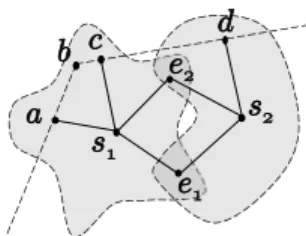
s1 s2 e1 e2 c d a b
Fig. 9. The approximation of covered region by a planar graph. The dashed lines show part of∂A. The dashed curves show the real sensing perimeters (unknown) of nodess1ands2.e1 ande2are two events detected by both of them.a,c, anddare points on the edges of∂Aintersecting the two sensing regions, andbis a vertex of∂A. Three faces,s1abcs1,s1e2s2e1s1, ands1cds2e2s1 are shown.
corresponding to the events detected by the node [15]. In this section, we consider how to compute the largest diameter of coverage holes if only a limited number of samples are known. To this end, we first construct a planar graph based on the samples observed. This graph is used to approximate the real covered region, that is, the union of all the sensing regions. We then show that under certain assumptions, the largest diameter of coverage holes can by estimated by the largest diameter of the faces of this graph.
LetBs denote the sensing region of nodes. We also use s to denote the position of nodes ande to denote the position where eventehappened. We make the following assumptions. 1) The positions of nodes and events observed are known. 2) Each Bs is a star convex subset of R2 with respect to
s, that is, any line segment joiningsto a pointt inBs, denoted asst, lies inBs. Figure 9 shows an example of two overlapped star-convex sensing regions.
3) For every connected component Ci ofBs1∩Bs2, s1=
s2, there is at least one event detected in each Ci, i.e., there is a point ei ∈ Ci known such that s1ei lies in Bs1 ands2ei lies in Bs2. For instance, the two sensing regions in Figure 9 intersect at two connected subregions, with one common event detected in each. 4) For each nodes, it is known whetherBs is completely
inside ofA, or is completely outside ofA, or intersects
∂A. In the last case, the set of edges of∂Athat intersect
Bsis known.
Let S denote the set of nodes whose sensing regions are within or intersect∂A, andEdenote the set of events observed by nodes inS . Let A denote the set of vertices of ∂A. For each node s ∈ S and each edge of ∂A that intersects Bs, pick an arbitrary point on that edge that is withinBs, such as points a,c, and din Figure 9. Name the set of such points
I. We construct a geometric graphG(V, E), whereV =S ∪ E ∪A∪I, and each edge in E corresponds to either a line segment joining a node s and an evente detected bys, or a line segment joining a nodesand a pointa∈Ion an edge of
∂A intersectingBs, or a line segment on ∂A joining points inAandI. See Figure 9 for reference. Notice that, the edges of Gmay intersect at points other than vertices. We makeG
planar by treating these intersections as vertices as well. We then observe thatGis a planar graph without open faces. LetD
andD denote the largest diameter of coverage holes and that of the faces of G, respectively. Then under the assumptions made above, we can observe that D≤D ≤D+ 2D, where
D is the maximum sensing diameter. We defer the proof of this statement to [4].
Notice that, the above approximation can also be applied to the case where all the sensing regions are known. It is not as accurate as the approach sketched in Section V-B, but more efficient since the faces ofGand their diameters can be easily computed. Ifd2D, the approximation may be desirable. In addition, if more events than required are detected, they can be used to improve the accuracy of the approximation.
VI. OPENPROBLEMS
Although we have addressed the problems of random de-ployment and algorithmic determination of the status of trap coverage, introduction of this new model of coverage opens up an opportunity to revisit several fundamental deployment and topology control problems afresh. First the problem of optimal deterministic deployment for various ranges of d
and r remains open. Second, the problem of joint coverage and connectivity (both from a deterministic deployment per-spective [2] and from an algorithmic perper-spective [12], [26]) remain open. Third is the problem of coverage restoration upon sensor failures [17]. Finally, the problem of sleep-wakeup [7], [13], [18], [29] which has traditionally assumed full coverage model or the barrier coverage model [19], also needs to be reinvestigated for this new model.
VII. CONCLUSION
This paper generalizes the traditional model of full coverage by allowing systematic holes of bounded diameter. With this new model, deterministic guarantees on detection, particularly tracking can be maintained even if not all points in the region are covered, whether due to failure of deployed sensors or due to the expense of deploying sensors to cover every point in a large region. Trap coverage thus makes sensor deployment scalable. Of independent interest is also the fact that the trap coverage model bridges the long-standing gap between the thresholds for percolation and for full coverage.
ACKNOWLEDGMENT
This work was sponsored partly by NSF Grants CNS-0721983, CNS-0721817, CCF-0728928, NIH Grant U01DA023812 from National Institute for Drug Abuse (NIDA), and FIT at the University of Memphis. The content is solely the responsibility of the authors and does not necessarily represent the official views of the sponsors.
REFERENCES
[1] R. Arratia, L. Goldstein, and L. Gordon, “Two Moments Suffice for Poisson Approximations: The Chen-Stein Method,”Annals of Probabil-ity, vol. 17, pp. 9–25, 1989.
[2] X. Bai, S. Kumar, D. Xuan, Z. Yun, and T. H. Lai, “Deploying Wireless Sensors to Achieve Both Coverage and Connectivity,” inACM MobiHoc, 2006.
[3] P. Balister, B. Bollob´as, A. Sarkar, and S. Kumar, “Reliable Density Estimates for Coverage and Connectivity in Thin Strips of Finite Length,” inACM MobiCom, 2007.
[4] P. Balister, Z. Zheng, S. Kumar, and P. Sinha, “Trap Coverage: Allowing Holes of Bounded Diameter in Wireless Sensor Networks,” University of Memphis, CS-09-001, Tech. Rep., 2008.
[5] S. Bapat, V. Kulathumani, and A. Arora, “Analyzing the Yield of ExScal, a Large Scale Wireless Sensor Network Experiment,” inIEEE ICNP, Boston, MA, 2005.
[6] Y. Bejerano, “Simple and Efficient k-Coverage Verification without Location Information,” inIEEE INFOCOM, 2008.
[7] M. Cardei, M. Thai, and W. Wu, “Energy-Efficient Target Coverage in Wireless Sensor Networks,” inIEEE INFOCOM, Miami, FL, 2005. [8] O. Dousse, C. Tavoularis, and P. Thiran, “Delay of intrusion detection
in wireless sensor networks,” inMobiHoc, 2006.
[9] Q. Fang, J. Gao, and L. J. Guibas, “Locating and Bypassing Routing Holes in Sensor Networks,” inProceedings of INFOCOM, 2004. [10] R. Ghrist and A. Muhammad, “Coverage and Hole-detection in Sensor
Networks via Homology,” inIPSN, Los Angeles, California, 2005. [11] C. Gui and P. Mohapatra, “Power Conservation and Quality of
Surveil-lance in Target Tracking Sensor Networks,” inACM MobiCom, 2004. [12] H. Gupta, S. Das, and Q. Gu, “Connected Sensor Cover:
Self-Organization of Sensor Networks for Efficient Query Execution,” in ACM MobiHoc, 2003.
[13] T. He and et al, “Energy-Efficient Surveillance System Using Wireless Sensor Networks,” inACM Mobisys, 2004.
[14] C. Huang and Y. Tseng, “The Coverage Problem in a Wireless Sensor Network,” inACM WSNA, 2003.
[15] J. Hwang, T. He, and Y. Kim, “Exploring in-situ sensing irregularity in wireless sensor networks,” inSenSys, 2007.
[16] V. Kulathumani, M. Demirbas, A. Arora, and M. Sridharan, “Trail: A Distance Sensitive Wireless Sensor Network Service for Distributed Object Tracking,” inEWSN, 2007.
[17] N. Kumar, D. Gunopulos, and V. Kalogeraki, “Sensor Network Coverage Restoration,” inDCOSS, Los Angeles, CA, 2005.
[18] S. Kumar, T. H. Lai, and J. Balogh, “On k-Coverage in a Mostly Sleeping Sensor Network,” inACM MobiCom, 2004.
[19] S. Kumar, T. H. Lai, M. E. Posner, and P. Sinha, “Optimal Sleep-Wakeup Algorithms for Barriers of Wireless Sensors,” inIEEE BROADNETS, 2007.
[20] M. Leonov, “Comparison of the different algorithms for Polygon Boolean operations,” http://www.complex-a5.ru/polyboolean/comp.html. [21] C. Sharp, S. Schaffert, A. Woo, N. Sastry, C. Karlof, S. Sastry, and D. Culler, “Design and Implementation of a Sensor Network System for Vehicle Tracking and Autonomous Interception,” inEWSN, 2005. [22] B. Tong and W. Tavanapong, “On Discovering Sensing Coverage Holes
in Large-Scale Sensor Networks,” Technical Report TR 06-03, Computer Science, Iowa State University, 2006.
[23] V. De Silva and R. Ghrist, “Coordinate-free Coverage in Sensor Net-works with Controlled Boundaries via Homology,”International Journal of Robotics Research, vol. 25, pp. 1205–1222, Dec. 2006.
[24] P. Wan and C. Yi, “Coverage by Randomly Deployed Wireless Sensor Networks,”IEEE/ACM Transactions on Networking (TON), vol. 14, pp. 2658–2669, 2006.
[25] G. Wang, G. Cao, and T. L. Porta, “Movement-Assisted Sensor Deploy-ment,” inIEEE INFOCOM 2004, Hong Kong, China, 2004.
[26] X. Wang, G. Xing, Y. Zhang, C. Lu, R. Pless, and C. Gill, “Integrated Coverage and Connectivity Configuration in Wireless Sensor Networks,” inACM SenSys, 2003.
[27] Y. Wang, J. Gao, and J. S. Mitchell, “Boundary Recognition in Sensor Networks by Topological Methods,” inACM MOBICOM, 2006. [28] C. Zhang, Y. Zhang, and Y. Fang, “Localized Algorithms for Coverage
Boundary Detection in Wireless Sensor Networks,”Wireless Networks, Feb. 2007.
[29] H. Zhang and J. Hou, “Maintaining Sensing Coverage and Connec-tivity in Large Sensor Networks,” in NSF International Workshop on Theoretical and Algorithmic Aspects of Sensor, Ad Hoc Wirelsss, and Peer-to-Peer Networks, 2004.
[30] ——, “On Deriving the Upper Bound ofα-Lifetime for Large Sensor Networks,” inACM MobiHoc, 2004.