ANDES: an ANalysis-based DEsign tool for
wireless Sensor networks
Vibha Prasad
∗, Ting Yan
∗, Praveen Jayachandran
†, Zengzhong Li
∗, Sang H. Son
∗, John A. Stankovic
∗,
J¨orgen Hansson
‡and Tarek Abdelzaher
†∗Department of Computer Science, University of Virginia, Charlottesville, VA 22904 †Department of Computer Science, University of Illinois Urbana-Champaign, Urbana, IL 61801
‡Software Engineering Institute, Carnegie Mellon University, Pittsburgh, PA 15213
Email:{vibha, ty4k, zl5r, son, stankovic}@cs.virginia.edu,{pjayach2, tarek}@cs.uiuc.edu, [email protected]
Abstract— We have developed an analysis-based design tool, ANDES, for modeling a wireless sensor network system and analyzing its performance before deployment. ANDES enables designers to systematically develop a model for the system, refine it iteratively by tuning the system parameters based on existing analysis techniques, and resolve key design decisions according to the required system performance. We also present a real-time communication schedulability analysis for sensor networks based on exact characterization which utilizes information regarding network topology and workload characteristics to analyze the schedulability of a set of periodic streams with real-time constraints. We further demonstrate the use of ANDES for the designers through detailed case studies where we design wireless sensor network applications (for target detection and environmental monitoring) using ANDES and validate the results through simulations.
Currently, ANDES supports communication schedulability analysis, target tracking analysis and real-time capacity analysis which work on system models with differing levels of detail. ANDES has been developed by extending the AADL/OSATE framework which has been used extensively for real-time and embedded systems. Based on key insights gained from the development of this analysis tool, we address issues in AADL for its use in the field of wireless sensor networks. We have developed a plug-in for ANDES, called ModelGeneration, which bridges the gap between the semantics needed for sensor networks and the syntax supported by AADL. This makes it easy for sensor network designers to build system models that are intuitive to them. Furthermore, ANDES is extensible and new analysis techniques can be easily incorporated into the toolset.
I. INTRODUCTION
Wireless sensor networks (WSNs) have recently gained a lot of attention because of their potential to have a huge impact on the way we live and society in general. WSNs are used for a variety of applications such as environmental monitoring, chemical plants, vehicle tracking, and smart healthcare. WSNs are composed of a large number of nodes, each of which have limited capability for sensing, processing, and communication. These nodes are deployed in real-world environments. Properly designing the WSN before deploy-ment is crucial and involves resolving trade-offs between many competing objectives. For example, increasing the number of nodes up to some density limit usually improves the performance of the system, but at the same time increases the cost of the system. Moreover, the system requirements
vary vastly from one application to another. For example, the main constraints in a military application [9] may be lifetime and real-time constraints, whereas in a healthcare application [21], privacy may have higher priority than lifetime.
There is a growing need for tools that aid system de-signers in performance tuning before system deployment. We propose an analysis-based design tool ANDES, which relies on offline analysis of the system model to help resolve design decisions. Theoretical analysis techniques are used to estimate key performance metrics (such as lifetime, sensing coverage, real-time capacity and reliability) of the system model based on a set of system parameters (such as the number of nodes, duty cycle, sensing range of nodes, and the available bandwidth). During the design process, these analysis techniques can be applied iteratively to tune various system parameters based on the desired performance and the performance estimated by the analyses. System param-eter tuning using theoretical analysis techniques have the attractive benefits of being inexpensive in terms of time and resources, better suited to large scale systems, and having a wider applicability and reusability across multiple deployments, as opposed to using simulation tools or system prototypes. Currently, ANDES supports target tracking anal-ysis, real-time communication schedulability analanal-ysis, and real-time capacity analysis, and we envision a larger suite of analysis techniques to be incorporated into ANDES in the future.
Our main contribution lies in introducing a design tool to a field like WSN where few existed, and providing a convenient mechanism for the designers to use theoretical analyses for design. Secondly, we develop a new real-time communication schedulability analysis which accurately determines the set of end-to-end streams that are schedulable within their dead-lines. Many WSN applications, especially those concerned with military surveillance, rescue squads, or fire detection systems have real-time constraints and would benefit from such an analysis. This new analysis models itself after the exact characterization schedulability analysis found in real-time computing. Finally, we present a case study to illustrate the use of analysis techniques in ANDES in the design of a sensor network, and validate the results obtained through simulations.
The remainder of the paper is organized as follows. We discuss the related work and the motivation for this work in Section II. In Section III, we explain our novel real-time communication schedulability analysis. In Section IV, we explain the other analysis techniques taken from the literature but implemented in ANDES, namely, target tracking analysis [3] and real-time capacity analysis [1]. The implementation of ANDES and the ModelGeneration plug-in support is discussed in Section V. In Section VI, we perform detailed case studies to demonstrate how ANDES can be useful for designers. We design a tracking-based application and an environmental monitoring application, and validate the results obtained from ANDES through simulations. We conclude and discuss future work in Section VII.
II. MOTIVATION ANDRELATEDWORK
Generally, designers of a WSN carry out simulations or evaluate the performance of a small prototype before developing the system. Various tools and services have been proposed in the literature to aid in-field testing and debugging [12], or performing simulation and emulation [7], [2], [18]. However, in-field testing requires at least a prototype system to be deployed and compared to simulations and prototyping, conducting offline analysis is inexpensive in terms of time and resources. At the same time, the accuracy of theoretical analyses depends on its assumptions and on how close the mathematical models assumed by the analysis are to the actual real-world scenario. Generally, simulators allow the designers to tune many different parameters and provide a fairly good resemblance of the real environment. Thus, theoretical analysis provides an alternate method of designing systems with lower cost and accuracy as compared to detailed simulation. Analysis-based design can be used along with simulation to evaluate trade-offs involved during system design.
Although theoretical analysis of WSNs is a relatively new area, there is a growing interest and new types of analysis are continuously being developed [3], [11], [23], [22], [1]. We believe that the attractive benefits of theoretical analysis towards system design will foster the development of a much needed theoretical foundation in the field of WSNs. Adding analysis techniques to design tools further has the advantage of providing the designers with the familiar and easy-to-use interface of the design tool while providing the benefits of theoretical analysis.
With respect to WSN systems, an analysis technique can be classified as an application level analysis or a system level analysis. Application level analysis techniques are specific for an application and assume a global view of the system, where the internal details of the WSN, such as the routing protocol, the energy level at each node etc., are hidden from the analysis and thus can be considered to be a part of the assumptions. System level analysis techniques operate at the system level and consider issues such as routing, communication model, group management protocols etc., depending on the level of abstraction provided by the system model.
From a designers’ point of view, it is desirable to start from a high-level model and incrementally add complexity to the model. Based on the results obtained from higher level analyses, the designers can fix certain system parameters (such as the node density, the duty cycle of the sensor nodes and the network topology) and move on to system level analyses. The designers can continue to choose other analysis techniques that focus on different sets of input sys-tem parameters and performance metrics. Suppose initially the designers want an estimate of the number of nodes to adequately cover a given area or to meet the desired quality of tracking (in a tracking-based application). After deciding on the no. of nodes and the topology of the network, the designers may be interested in estimating the capacity of the network or evaluating various routing protocols. At a lower level, the system model can further be integrated with an energy model, which considers transmission cost, reception cost and computation cost, to determine the expected lifetime of the system. Using this energy model, the system designers may further want to understand the effect of data aggregation on schedulability or estimate the reliability of the current system. Note that at each step we are getting closer to the actual implementation of the WSN. Thus, the system model can be refined iteratively by performing analysis at each level of abstraction/granularity. Ideally, the final model should cover as many design decisions as possible using the available analyses.
We used the AADL/OSATE framework for ANDES. AADL/OSATE has been widely used for real-time and em-bedded systems and provides a component-based framework for modeling hardware and software components as well as the interaction between these components. More importantly, AADL/OSATE offers several analysis plug-ins for embedded and real-time systems which can be used for WSNs. Some examples of the available analyses and consistency checks are required connection checking (which ensures that some ports are always connected), flow latency analysis (which checks the latency of flow implementations with respect to the flow specifications) and resource allocation and budget analysis (which allows users to perform resource budgeting for processors, memory and network bandwidth and analyze whether the capacity is exceeded by the budgets). Thus, AADL/OSATE is an ideal platform for WSN systems which involve a very close interaction between the hardware and software components and can benefit from the existing sup-port offered by AADL/OSATE.
Design frameworks other than AADL/OSATE could be used, but using AADL has several advantages over other existing design tools such as the following. Tools like VEST [16] and Cadena [8] have been developed in academia, but are not as widely used nor as mature as AADL. There are several UML-based tools like Rhapsody [15], but UML [10] does not support precise semantics and is not used specifically for real-time and embedded systems. Tools like TimeWiz [19] and STOOD [17] are proprietary and MetaH [20], developed by Honeywell, is the predecessor of AADL.
There are a few other design tools for WSNs, but their motivation and approach is different from ANDES. Tinker [4] is a high-level design tool for sensor networks which uses actual data streams from the deployment site to decide on data processing algorithms. Various algorithms can be compared to find the one that gives the best result for the given application. Unlike Tinker, ANDES does not use data to guide its decisions. It uses an analysis-based design approach to decide on the system configuration. However, ANDES can be extended to include data-driven analysis where real-world deployment data is used to tune the system model. Integrating data processing algorithms with ANDES can be part of the future work. SensDep [14] is a design tool for WSNs which considers the trade-off between coverage and the cost of the system. This is closer to the work presented through ANDES. SensDep considers mobility and differential surveillance requirements. The optimal solution presented in the paper works for small scale systems only and is based on integer mathematical programming. The heuristic solutions work by generating a list of deployment patterns and matching the deployment patterns that perform well with devices. Currently, ANDES does not support such an analy-sis. However, such an analysis can be easily incorporated in ANDES.
Both the tools help the designers in understanding the system better and develop a model in a more informed manner. However, using ANDES has additional benefits. The AADL system model can be used as a document for inter-action among the designers, clients and developers through all phases in the software lifecycle. Building architectural models allows the designers to early on and throughout the development cycle establish assurance of a system design, and conduct impact and trade-off analysis, e.g., with respect to performance, security, and dependability. As the models are incrementally augmented with system details and pa-rameters, the designers can establish increased assurance of the quality attributes of the system design. In addition to improving the quality and predictability of the system design, this achieves a considerable reduction in the cost (time and money) of testing and maintenance.
The existing work on WSN analysis consists of isolated efforts and the analyses are usually geared towards a specific application. Our vision of ANDES consists of a design framework for WSNs that not only has the support provided by AADL/OSATE, but also integrates these isolated efforts into a repository of analyses which are at the designers’ disposal. This unified framework will provide the designers with ample choice which would not have been available otherwise. The designers can use the wealth of knowledge available in the AADL/OSATE framework and through the repository for modeling and validation of WSN systems. At the same time, it is crucial for the success of such a tool not to compromise on the convenient, easy-to-use and intuitive interface for the designers.
III. COMMUNICATIONSCHEDULABILITYANALYSIS
The main goal of the real-time communication schedu-lability analysis is to find out if a schedule for multi-hop end-to-end communication streams is able to meet the deadlines of all the streams in the system under given assumptions. This problem is NP-hard [11], we develop and evaluate three offline heuristic algorithms with different scheduling granularity and problem scale. We model our solutions after the exact characterization method employed in real-time scheduling theory. Although, many asymptotic throughput analyses for WSNs exist in the literature, they only consider the general throughput bounds and do not utilize information regarding the network configuration and the workload characteristics, if they are known beforehand. We assume complete knowledge of the network configu-ration and workload characteristics and focus on periodic streams with explicit time constraints, instead of dealing with bit-level workloads. In developing the communication schedulability analysis, we were motivated by the grow-ing number of WSN applications with real-time constraints (military surveillance systems, fire detection system, volcano monitoring etc. ) and the lack of analysis techniques on communication schedulability which take interference among sensor nodes into account. The communication schedulability analysis is especially suited for such applications where the throughput analysis may be too pessimistic in its evaluation. The designers can perform the throughput/capacity analysis to understand the communication capabilities of the system and refine the design to include information regarding the network topology and workload characteristics to analyze the system using the communication schedulability analysis. This information can come from constraints imposed by the application requirements (e.g. on the period of streams), or the deployment environment (e.g. on the network topology), or from previous experiences. In this section, we explain the three algorithms, Stream-Major, Link-Major and Time-Major algorithms and evaluate them in Section VI-D. For further details, the reader can refer to [11].
All communication links are assumed to be symmetric. For successful transmission, the receiver should lie within the sender’s radio range and no other sender should lie within the interference range of the receiver. It is also assumed that the receiver’s interference range is not less than the radio range of the receiver, which is true for most wireless scenarios.
The analysis defines streams as periodic end-to-end data transmissions which need to traverse from source sensors to destination sensors via multiple hops. Every stream is characterized by an ordered tuple, Stream Vector = (Deadline, Period, Start Time, Transmission Delay, Routing Path). The Deadline is the maximum duration of time starting from inception of a packet of the stream, within which the packet’s end-to-end transmission needs to be completed. The Period defines how frequently the stream regenerates. A new in-stance of the stream is generated after each period. The Start Time is the time when the timer starts counting down for the Deadline. The Transmission Delay is the time taken for
data sensor data end sensor data;
property set wsn property is
grid size: aadlinteger applies to (system); .
. .
node no: aadlinteger applies to (device); end wsn property;
device Node features
in port: in data port sensor data; out port: out data port sensor data; flows
flow source: flow source out port ; flow path: flow path in port−>out port; flow sink: flow sink in port;
end Node;
device implementation Node.node0 properties wsn property::node no=>0; end Node.node0; . . . system wsn end wsn; system implementation wsn.wsn1 subcomponents
node0: device Node.node0; .
. . connections
conn14: data port
node1.out port−>node4.in port; .
. . flows
stream1:
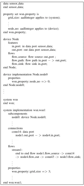
end to end flow node1.flow source ->conn14 ->node4.flow out ->conn43 ->node3.flow sink; . . . properties wsn property::grid size=>3; . . . end wsn.wsn1;
Fig. 1. A Simple AADL Program with streams
one hop transmission and is assumed to be the same for the entire path of the specific stream. The delay can be used to account for the unreliable nature of the wireless medium. The Routing Path is a list of communication links through which the data is transmitted in order to reach the destination node. An internal data structure called the link allocation table is used for the analysis, where the rows represent all the communication links in the network and the columns represent time slots. A time slot represents the number of time units for a single packet transmission. A table entry represents the status of the communication link (free, allocated, blocked) in a given time slot.
The basic scheduling strategy followed by the heuristic algorithms is as follows:
1) Find and choose the most important stream based on scheduling heuristics.
2) Find and allocate free link entries to the stream taking interference into account.
3) Update every stream’s importance upon the changes
made by the new allocation.
4) If there are streams waiting to be scheduled, return to step 1.
The scheduling heuristic determines which stream should be scheduled in the current scheduling step. The heuristic can be a static heuristic (based on deadline, period or total no. of transmission hops), that do not change during the scheduling process, or dynamic heuristics which may change in every scheduling step. Dynamic heuristics can further be divided into Urgency-First and Throughput-First heuristics. Urgency-First heuristics give higher priority to streams that are closer to their deadline. Throughput-First heuristics try to maximize the channel use. Furthermore, there are three urgency metrics of interest, earliest start time, laxity, and velocity, which reflect different properties of the network and the workload. Earliest start time (EST) is the earliest time slot which is available to the stream such that there are enough continuous unoccupied and non-interfered free entries in the link allocation table to be allocated for the stream’s next requested communication link. EST not only depends on the stream’s preceding state, but also on other streams’ states as one stream’s transmission interference may delay the other streams. Thelaxityof a stream represents the delay (in terms of time slots) it can tolerate in the remaining transmissions and it can be calculated as: Laxity = Start Time + Deadline - Remaining Hops × Transmission Delay - EST. Streams with lower value of laxity are more urgent. Adding EST to the calculation of laxity increases its accuracy.
Velocity indicates the stream’s required transmission speed and can be calculated as: Velocity = Remaining Hops/(Start Time + Deadline - EST). Thus, streams with larger velocities have higher urgency. A similar throughput heuristic is hard to quantify because of the NP-Hard nature of the problem. However, we can associate aninterference indexwith every requested communication link, which indicates the number of links with which this link interferes. A heuristic solution for the throughput optimization can be obtained by choosing the stream with the smallest interference index.
Scheduling the different streams in the network occurs in a sequence of scheduling steps, where each schedul-ing step represents a run of the schedulschedul-ing heuristic. The Stream-Major algorithm schedules one entire stream in every scheduling step using laxity as its urgency metric. The Link-Major algorithm schedules one individual link in every scheduling step using laxity as its urgency metric. Note that although laxity is being used as the urgency metric, EST has to be calculated in every scheduling step. The Time-Major algorithm allocates link entries for one time slot in every scheduling step. It is motivated by the Throughput-First heuristic which aims at scheduling multiple simultaneous transmissions. Among these three algorithms, Stream-Major has the least number of scheduling steps as it schedules all instances of a stream in each scheduling step. The scheduling granularity of Stream-Major algorithm is still coarse as compared to the other algorithms, as it does not consider the individual priority of the stream instance and schedules
the entire stream at once. The number of evaluations of the heuristic that are needed are of the order of O(N2), where N is the number of streams. In contrast, Link-Major has the maximum number of scheduling steps as it schedules one link of one active instance of a stream in each scheduling step. It is supposed to have the highest scheduling precision among these three algorithms as it schedules one transmission of one instance of a stream in every scheduling step. The total number of evaluations of the heuristic needed are of the order of O(N ×I×H2), where N is the number of
streams, I is the average number of instances per stream, and H is the average number of transmission hops per stream. The Time-Major heuristic involves fewer scheduling steps than the Link-Major heuristic as it schedules multiple transmissions in one scheduling step. For Time-Major, the total number of evaluations isO(SchedulingLength), where
SchedulingLengthis the number of columns needed in the
link allocation table.
The schedulability analysis is designed for cases where the designers have a detailed knowledge of the system. More specifically, the designers should have sufficient information about the expected workload in the system. This is dependent on the application. For example, suppose in a WSN fire alarm and rescue system, all the sensor nodes send data periodically back to the base station (and have a sleep cycle to conserve energy). However, in case of a fire, all nodes wake up and send data with a smaller period back to the base station. This data can be used to rescue people in the building. In those crucial moments, it is necessary that no data is lost in transition and the information reaches within a deadline. Using the communication schedulability analysis, the designers can evaluate the performance of the system for average as well as worst case workloads. Figure 1 shows the system model required for the communication schedulability analysis, which has much more detail than the tracking analysis (Figure 2). Note that a sensor node participating in a stream can either pass data or act as a source/sink of data (flows in device Node). One of the end-to-end streams, stream1, is shown, where the data flows from node1 to node3 via node4 (using conn14 and conn43).
IV. ANALYSISTECHNIQUES INANDES
Currently, we have developed plug-ins to support three analyses: target tracking analysis [3], real-time capacity anal-ysis [1] and real-time communication schedulability analanal-ysis (described in Section III). To fully understand the value of the tool, in the following subsections, we briefly explain the theory behind the tracking analysis and the capacity analysis implemented in ANDES. Since the tool is extensible, over time, key analysis techniques from the literature can be added. Including these two solutions here demonstrates this capability. Further, implementing these three analyses as plug-ins, enables us to compare the system models needed for these analyses and derive the issues that need to be addressed in AADL.
property set UVAWSN is
WSN Period: aadlreal applies to (system); WSN DutyCycle: aadlreal applies to (system); WSN SensingRange:
aadlreal applies to (system);
WSN Density: aadlreal applies to (system); TARGET Speed: aadlreal applies to (device); TARGET FromOutside:
aadlboolean applies to (device); end UVAWSN; system WSN end WSN; device TARGET end TARGET; system implementation WSN.WSN1 properties UVAWSN::WSN Period=>1.0; UVAWSN::WSN DutyCycle=>0.1; UVAWSN::WSN SensingRange=>10.0; UVAWSN::WSN Density=>0.016; end WSN.WSN1;
device implementation TARGET.TARGET1 properties
UVAWSN::TARGET Speed=>20.0; UVAWSN::TARGET FromOutside=>true; end TARGET.TARGET1;
. . .
Fig. 2. AADL system model for Tracking Analysis A. Tracking Analysis
The main goal of the tracking analysis [3] is to predict surveillance performance attributes, represented by the de-tection probability and average dede-tection delay of intruding targets, based on tunable system parameters, the node density and sleep duty cycle of the WSN. The analysis considers stationary, slow moving and fast moving targets through the network. The authors have also evaluated the sensing model and shown that the results are robust to a realistic sensing model.
The AADL system model needed for the tracking analysis is shown in Figure 2. There is one WSN system implemen-tation and several implemenimplemen-tations for external targets. This model needs a few properties: node density(d), period(T), sensing range(R) duty cycle (β, the fraction of the time period the nodes stay awake) and width(L, length of the target path in the network) to describe the WSN and speed(v) and direction of the target (whether the target is inside the network or is coming from outside the network) to describe the target.
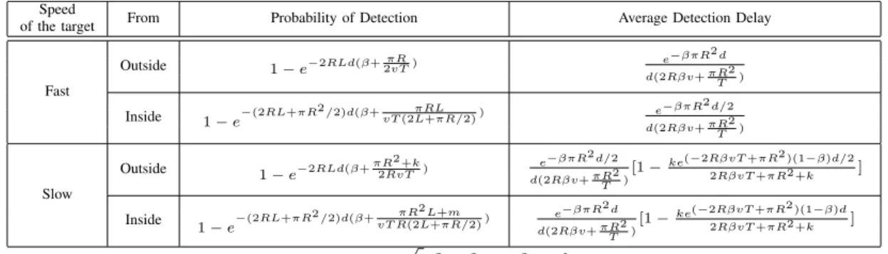
Table I summarizes the results obtained in the tracking analysis. For their derivations and further details, we refer the reader to [3]. The tracking analysis is very useful for the designers of a tracking-based applications as the sensing quality is directly related to deployment choices.
B. Real-Time Capacity Analysis
Real-time capacity for wireless sensor networks was first analyzed in [1], where real-time capacity of a sensor network is defined as the bit-distance product of all messages deliv-ered by the network, normalized by their relative deadlines. This definition is intuitive as it can be expected that the network can deliver more bits when the deadlines are larger,
Speed From Probability of Detection Average Detection Delay of the target Fast Outside 1−e−2RLd(β+2πRvT) e−βπR2d d(2Rβv+πRT2) Inside 1−e−(2RL+πR2/2)d(β+vT(2πRLL+πR/2)) e−βπR2d/2 d(2Rβv+πRT2) Slow Outside 1−e−2RLd(β+πR2+k 2RvT ) e−βπR2d/2 d(2Rβv+πRT2)[1− ke(−2RβvT+πR2)(1−β)d/2 2RβvT+πR2+k ] Inside 1−e−(2RL+πR2/2)d(β+ πR2L+m vT R(2L+πR/2)) e −βπR2d d(2Rβv+πRT2)[1− ke(−2RβvT+πR2)(1−β)d 2RβvT+πR2+k ] where a= (1−β)vT /2,k= 2a p (R2−a2)−2R2cos−1(a R),m= (L−a)k TABLE I
RESULTS OBTAINED FROMTRACKING ANALYSIS
and when the distance traversed by messages is shorter (exploiting spatial diversity). For a load-balanced sensor network, the real-time capacity was obtained as:
CRT =
nα
2mNW (1)
wherenis the number of nodes in the network,mis called the node density parameter defined as the average number of neighbors a node can transmit to, N is the maximum hop length of any message, W is the transmission rate, and
α is called the urgency inversion parameter defined as the minimum ratio of the deadline of a message to that of any higher priority message.
For more realistic multihop sensor network traffic patterns where a small number of sinks collect sensor readings from all the sensor nodes (also known as convergecast traffic), a real-time capacity expression is derived in [1] as:
CRT = αKNk
2 + lnNkW (2)
where K is the number of sinks, and Nk is the maximum
source-to-sink hop count.
In our implementation, the designer can either calculate the real-time capacity given the above system parameters, or conversely can estimate the number of sinks required to ensure a minimum specified capacity.
V. IMPLEMENTATION OFANDES
In this section, we describe how ANDES fits in the AADL/OSATE framework and discuss several issues in us-ing AADL for developus-ing WSN system models. We use the communication schedulability analysis to illustrate these shortcomings and suggest modifications to be included as part of ModelGeneration.
The SAE1AADL (Architecture Analysis and Design
Lan-guage2) is an international standard for predictable
model-based engineering of real-time and embedded computer sys-tems. AADL is very popular in industry as well as academia and many analysis tools for real-time embedded systems use AADL to conduct impact and trade-off analysis, e.g., with respect to performance, security, and dependability.
1Society of Automotive Engineers
2Formerly known as Avionics Architecture Description Language
AADL offers a set of predefined component categories [5] to represent real-time systems and it is capable of describing functional interfaces to components like dataflows and con-trol flows as well as non-functional aspects of components like timing properties.
OSATE (Open Source AADL Tool Environment) is an Eclipse-based open source framework that is a front-end AADL parser and generator. AADL models are developed in OSATE and an intermediate representation (an XML representation, AAXL) is generated. The XML representation allows interoperability and integration with other commercial and in-house tools. The interaction between the OSATE framework, the analysis plug-ins, ANDES, and the AADL system models is shown in Figure 3. The analysis plug-ins are written in Java and are built on top of the OSATE framework. ANDES is invoked as the runtime Eclipse application and AADL system models are built on the ANDES framework. Analysis techniques can be invoked from ANDES to analyze the system models. The plug-in nature of OSATE allows it to be extensible and hence ANDES can be easily extended to add other analysis techniques.
From a designers’ perspective, the learning curve involves learning AADL, which is a component-based modeling lan-guage with pre-defined components for modeling hardware, software and their interactions. From our experience, AADL has a clean syntax which is easy to learn. However, if the designers wish to add more analyses to ANDES, it involves more effort. In particular, it requires the designers to be familiar with the OSATE plug-in development environment and necessary support plug-ins. The plug-ins themselves are written in Java.
In our experience with AADL for WSNs, we encountered many instances where AADL did not have a convenient solution for modeling WSNs. The main challenges were in achieving scalability (sensor networks typically have hun-dreds or even thousands of nodes), specifying the connec-tivity among nodes, and the coverage shape of WSNs. We have addressed these issues in ANDES by developing a plug-in (ModelGeneration) which bridges the gap between the semantics needed for sensor networks and the syntax supported by AADL. We list the main issues with AADL faced by the system designers of WSN systems and the solution proposed by ModelGeneration as follows:
• Scalability: In real applications, it is not unusual for a
WSN system to have hundreds or thousands of nodes, thus it is essential for the interface of the design tool to be simple and easy-to-use, and scale well even for large-scale systems. To model a large-scale system with many nodes, currently3 the component implementation
of each of these nodes has to be defined individually. ModelGeneration Solution For Scalability:TheWSN coverage shapeis the shape of the deployment area. In ANDES, WSN coverage shapes such as grid, random, rectangular and T-shape can be expressed and we discuss their implementation later in this section. The number of nodes in the system is represented by using three
properties: grid deployment, grid size, and
active nodes. grid deployment is a boolean property which is true if the WSN coverage shape is a grid and false otherwise. grid size represents the size of the grid where the grid is a square of
edge length grid size. active nodes represent
the number of nodes active in the grid, and is useful when the nodes are distributed according to a WSN coverage shape other than a grid. For example, suppose the system model contains component implementations for m sensor nodes, such thatm≤active nodes, and the nodes are distributed according to a WSN coverage shape other than a grid. This means that the system contains (active nodes−m) more nodes which have not been declared in the system model and hence should be added by ModelGeneration according to the specified coverage shape.
• Connectivity: First, all the connections for each
node have to be explicitly laid out for the analysis. A connection is a communication link between two sensor nodes. If we consider an n×n grid, where each of the nodes is connected to its immediate neighbor on all four sides, the total number of connections in the network is Θ(n2). Secondly, there is no easy way of
specifying wireless connections based on a given radio range and interference range. It is not intuitive to use the component type bus, which is used extensively in AADL to allow access to processor, memory, devices
3It has been agreed by the AADL Subcommittee that AADL v2 will
include constructs for arrays and templates that support representation of multiplicity.
etc., for wireless systems. Finally, it is not possible for designers to specify the end points of the stream and determine the feasible set of routes for the streams in the WSN. In AADL, the details of the stream have to be specified by the designers as a flow path.
ModelGeneration Solution For Connectivity: For specifying connectivity between nodes, we use the
prop-erties radio range and interference range.
All nodes within the radio range of a node
are connected to it. Any transmission within the interference range of a node, interferes with transmissions to that node. The connections between nodes are calculated using these properties and added to the system.
Streams are represented by the keyword flows in AADL. ModelGeneration enables the user to specify a high-level description of end-to-end streams by using
the keyword device which has source node no
andsink node noas its properties. This is especially useful if the analysis can intelligently change the route of the streams based on the end points and the result of the analysis (i.e. if the streams are schedulable or not).
• WSN Coverage Shape:Specifying each node location
through the node numbers or grid positions is not intu-itive for the designers when the nodes are not deployed in a grid. It is much easier if there is a way to specify the WSN coverage shape (rectangular, circular, T-shaped etc.) as a whole and declare some special parameters associated with it which specify it completely.
ModelGeneration Solution For WSN Coverage Shape: Currently, we have support for modeling grid, randomly distributed, rectangular and T-shaped WSN coverage shapes. More WSN coverage shapes can be added to ANDES based on what is needed by the analysis. The WSN coverage shape is specified by the parameters topology, length, width and border. Each WSN coverage shape that is implemented is assigned a unique number to denote its topology. Length, width and border are specific to the WSN coverage shape. Although, AADL consists of a textual as well as a graphi-cal language for modeling the system architecture, currently, flows cannot be depicted graphically in OSATE. Since flows are an important aspect of the system models used in this paper, we were unable to illustrate graphical models of the system. This problem should be addressed by OSATE in future. Graphical AADL models improve the ease of use of ANDES.
VI. CASESTUDIES ANDEVALUATION
In this section, we design simple sensor network sys-tems using ANDES and validate the design decisions us-ing simulations. In Sections VI-A and VI-C, we design a target tracking application and an environmental monitoring application, respectively. We evaluate the design decisions for the application in case study 1 in Sections VI-B. The main motivation of such an evaluation is to demonstrate
(a) (b) Fig. 4. Designing a Tracking-based WSN System (node density = 0.015)
the usability of ANDES and quantify the accuracy of the recommendations made, which depend on the incorporated analyses. Due to lack of space, we have not included the evaluations for case study 2. In Section VI-D, we evaluate the communication schedulability analysis. We have also evaluated ANDES in terms of the convenience offered to the designer by comparing the lines of code (LOC) needed for the WSN system models. For further details, the reader is referred to [13].
A. Case Study 1: Designing a Tracking-based Application
In this section, we design a target tracking application. The task of the system designers is to design an application for the surveillance of a100m×100marea. The designers can use a maximum of200sensor nodes, each having a sensing range of 10m and a transmission range of 20m. The sensors are deployed in a uniform random manner, which is realistic for many surveillance applications. We make two assumptions in this scenario. Our first assumption is that only one message stream is generated per target. This can be implemented using an appropriate group management protocol. Among a group of nodes that detect the target, one node can be designated as the group leader and can communicate with the base station. Our second assumption is that after the target is detected, the group leader sends periodic messages (0.25Kbof data every half a second) until the target is out of its sensing range. At that time, a new group leader can be appointed. The sensor nodes can transmit at a rate of20Kbps.
The requirements for the system performance are as fol-lows. The system must be able to detect targets 99% of the time, for all mobile targets.The system is required to have a maximum average target detection delay of 1s for fast moving targets and2sfor slow moving targets. For the tracking analysis, we assume that we are interested in targets moving at speeds around 2.5m/s (which are considered to be slow moving targets) and those moving at speeds around 25m/s (which are considered to be fast moving targets). Moreover, the system should be able to support5concurrent targets in the average case and up to 20 concurrent targets in the worst case. Taking these constraints into account, our task as system designers is to design a sensor network to
meet these requirements.
As described in Section II, we start with an application level analysis (the tracking analysis) and then add sophis-tication to the design using a system level analysis (the capacity analysis). The system parameters that can be tuned using the tracking analysis are node density and duty cycle. Since we have a predetermined area, reducing the node density reduces the number of nodes and hence the cost of the system, but would negatively affect the target detection probability and detection delay. Likewise, reducing the duty cycle gives higher energy savings, but would decrease the detection probability and increase the detection delay. We therefore need to determine the minimum values for node density and duty cycle that would ensure that the performance requirements are satisfied. After identifying the required node density and duty cycle using the tracking analysis, we demonstrate how these values can be used by the capacity analysis to compute the minimum number of base stations that would be required to ensure enough capacity in the system to detect and report20concurrent targets.
In order to demonstrate how the performance requirements vary with the tunable system parameters, we show the varia-tion of the probability of detecvaria-tion and the average detecvaria-tion delay with duty cycle, when the node density is fixed at 0.015, in Figures 4(a) and 4(b). We can observe from these figures that the probability of detection increases monotonically with the duty cycle and the average detection delay decreases with increasing duty cycle. The probability of detection degrades faster with decreasing duty cycle for faster targets. For one case (slow targets coming from outside the sensor field), the detection delay is higher at low duty cycle as compared to others. This is due to the combination of two factors. Firstly, slower targets may move a very short distance in a sensing range, therefore, they may be go undetected for a longer time when the duty cycle is low. Moreover, there may be an added delay in the case of outside targets as the edges of the sensor field may not be covered that well. This becomes more pronounced in the case of slow targets. For a node density
of0.015, although the probability of detection is more than
99%, the average detection delay for slow moving targets coming from outside is not less than2sfor duty cycle<0.4.
This demonstrates that it is indeed quite difficult for the designer to manually adjust and estimate even near-optimal values for the node density and duty cycle, that would meet the performance requirements.
The analyses described in this paper estimate some per-formance metric given values for various system parameters. However, typically the designers are interested in estimat-ing suitable values for tunable system parameters, given minimum (or maximum) performance requirements. This functionality has been added for target tracking analysis and real-time capacity analysis. Instead of manually adjusting the tunable system parameters and getting values of the performance metrics for every system configuration, the designers can alternatively specify the desired performance requirements. In that case, ANDES determines values for the tunable system parameters that best satisfy the requirements and displays them in a tabular form. This is an efficient mechanism to obtain an estimate of the system parameters. For this case study, we obtained results for targets with velocities between5m/sand25m/sentering the sensor field from outside. For different values of node duty cycle, these results provide the minimum density of node deployment required to satisfy the performance requirements. We see that the slow target from outside can not be detected within the desired performance criteria for duty cycle lesser than 0.4 (the tool returns “No Solution” for these values). From these results, the designers may select the values of duty cycle as 0.4 and node density as0.015 nodes/sq. meter and obtain results4. This functionality, where the designers can
obtain an initial estimate of the system design parameters from the desired system performance, enables the designers to use ANDES efficiently.
A node density of 0.015 nodes/sq.meter in a100m×100m
field implies a deployment of 150 nodes. Based on our assumptions that nodes are deployed uniformly at random and each node has a transmission radius of 20m, it is reasonable to assume that the maximum number of hops from any node to a centrally located base station is 6.
We now conduct the capacity analysis to compute the number of base stations needed by the system to support 20 concurrent targets, with each target generating 0.5Kbps
of data. As each stream needs to be carried for a maximum of 6 hops, the total required capacity of the system can be calculated as 20×0.5×6 = 60Kb−hops/sec. With a capacity requirement of60Kb−hops/secand a transmission rate of 20Kbps, ANDES estimates the required number of sinks (K) as 2 using the capacity analysis (the result can be determined using Equation 2).
Using this case study, we have shown how designers can use ANDES to get recommendations based on analysis of the system model. While the actual performance of the system depends on external factors and the accuracy of the assumptions made, going through this process is extremely
4When the duty cycle and node density values are fixed at0.4and0.015
nodes/sq.m respectively, the probability of detection and average detection delay for a target with velocity25m/sis0.999and0.059srespectively.
valuable for the designers in understanding the impact of the system parameters on the performance. We validate this design in the next subsection.
B. Evaluation of Design Decisions: Case Study 1
In this section, we evaluate the design decisions obtained for case study 1 (tracking and capacity analysis) through simulations. We used a C++ based simulator obtained from
Cao et al. [3].
Fig. 5. Comparison of Tracking Analysis and Simulation results
Figure 5 shows the results obtained from analysis and those obtained from simulation for the average detection delay with varying target velocity. We conducted 100 rounds of simulations. In each of these rounds, the locations for 150 nodes and20targets are generated. The detection delay was measured for every target and Figure 5 shows the average detection delay for 100 rounds of simulation with the 95% confidence level. In our simulations, the sensing range is not uniformly circular. It is based on actual readings from the PIR sensors [3]. From the graph, we observe that the detection delay meets the original performance requirements, as it is less than 2s for target velocities varying from 2.5m/s to 10m/s (slow targets) and less than 1s for target velocities varying from 10m/sto30m/s(fast targets).
10 20 30 40 50 60 70 80 90 100 30 25 20 15 10 5
Real-Time Capacity (Kbit-hops/s)
Transmission rate (Kbps) Simulation
Analysis
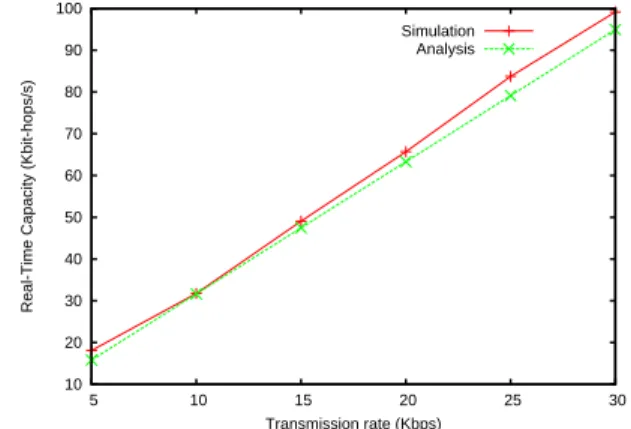
Fig. 6. Comparison of real-time capacity obtained from analysis and simulations for different values of transmission rate
As in [1], we used a customized simulator to study the capacity of wireless sensor networks. Nodes were assumed to be placed uniformly within the field and flows were generated
by choosing sources uniformly at random and transmitting packets to the nearest of two sinks. Prioritized scheduling was implemented within each node, such that packets belonging to a flow of higher priority would always be transmitted ahead of packets of a lower priority flow. Since we are interested in the maximum sustainable capacity, a lossless MAC layer was assumed. For the scenario described, the minimum capacity of the network at which a deadline miss was observed was noted as65.70Kbit−hops/second (this was the minimum from 50 randomized runs). In Figure 6, we plot the capacity of the network obtained from simulations and analysis for different transmission rates ranging from5Kbpsto30Kbps. The actual maximum capacity of the network is expected to be better than this value as the routing used for this simulation was shortest-path routing, and if the intended recipient of a message is blocked due to another transmission, the packet was not scheduled until that transmission was over. With smarter routing protocols, it is possible to transmit the packet to an alternate free node so that progress can be made towards the sink node without being blocked.
C. Case Study 2: Designing an Environmental Monitoring Application
In this section, we use ANDES to design an environmental monitoring application. For this application, the sensors are deployed in a 5 ×5 grid, with a grid spacing of 10m. Each sensor node is equipped with many sensors such as temperature, humidity, and light. All the sensor nodes send data from its sensors (of message length0.5Kb) periodically every minute to the base station. The radio range of the sensor nodes is12mand the interference range is25m. In a grid, this means that every node has four neighbors, and the maximum number of hops from any node to a centrally located base station is 4. We assume that the nodes can transmit at a rate of25Kbps. Our main assumption in this case study is that the data are not aggregated at any point. Each node is a source of a stream of data to the base station.
We first use the capacity analysis to find the number of base stations required to support concurrent streams from all the nodes in the system. The number of hops that each message traverses before reaching the destination varies between 1 and 4, and the average number of hops can be taken as 2.5. The maximum required capacity is therefore
24×2.5×0.5Kbps= 30Kb−hops/s (at least one node
would act as a base station, and would therefore not create any traffic). With a maximum of 4 hops from any node to a base station, and nodes transmitting at 25Kbps, from the capacity analysis we find that one sink is sufficient for this network.
The schedulability analysis uses more detailed knowledge of the system to compute if the streams are schedulable within their deadline. We place the base station at the center of the 5×5 grid. With the given specifications, 24streams were generated from all the sensor nodes to the base station. The period and deadline were set at60s. The schedulability analysis reported that all streams will be schedulable within
their deadlines. Due to lack of space, we have not included the evaluation of this case study using simulations in this paper. Instead of evaluating schedulability analysis for this specific case, we discuss a more general evaluation for schedulability analysis in Section VI-D.
D. Evaluation of Communication Schedulability Analysis
In this section, we evaluate the three heuristic algorithms Stream-Major, Link-Major and Time-Major, for a more gen-eral design. The performance of these algorithms is evaluated with respect to the workload (number of streams) and the network size. We have evaluated the algorithms using MatLab and used “Fraction of Streams Scheduled” as the evaluation metric. The WSN topology is assumed to be a10×10grid of nodes with a grid spacing of 10m. Ten pairs of source and sink locations are generated randomly and twenty routes are generated for every pair constituting the twenty sets of streams. For all the streams, the deadline is equal to the period and the period is the same for all (20s). The radio range is 12mand the interference range is25m.
Fig. 7. Schedulability Analysis Results: Effect of Stream Workload
Figure 7 shows the variation of the fraction of scheduled streams with the number of streams. The performance de-grades quickly as all streams have the same periods and there is a higher probability of the streams getting delayed because of interference. We can see that despite its coarse granularity Stream-Major is able to keep up with Link-Major. Time-Major has the lowest fraction of scheduled streams among the three, however, it catches up when the number of streams becomes larger. The reason for this could be that Time-Major is not able to schedule many links simultaneously in a dense network due to interference.
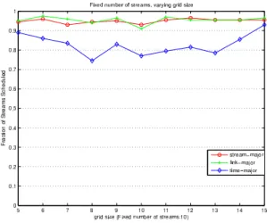
Figure 8 shows the variation of the fraction of scheduled streams with the grid size. The number of streams is fixed
at10. Time-Major performs the worst among the three and
it shows the highest variance. Stream-Major and Link-Major consistently perform above90%. The results show that Time-Major is the most sensitive to the location of streams in the workload.
Fig. 8. Schedulability Analysis Results: Effect of Grid Size
VII. CONCLUSIONS ANDFUTUREWORK
In this paper, we have presented an analysis-based design tool, ANDES, for WSNs with the AADL/OSATE framework. We have highlighted a few issues with AADL syntax that does not adequately cater to semantics needed for WSN modeling. We have developed a new real-time communi-cation schedulability analysis that accurately determines the set of end-to-end streams that are schedulable within their deadlines. In addition to the communication schedulability analysis, we have also implemented a tracking analysis and a real-time capacity analysis in ANDES. Finally, we demon-strate the usage of ANDES through detailed case studies.
An important open research question is determining the proper set of analysis techniques that must be developed together with an understanding of their interactions in order to make design tools like ANDES sufficient for designing WSNs. We believe that for completeness the analytical toolset should at least cover lifetime, reliability, sensing coverage, real-time capacity, scheduling, quality of service, and security issues.
ACKNOWLEDGMENTS
We thank Aaron Greenhouse for his timely help with AADL/OSATE. This work was supported in part by SEI 06-00423 and NSF grants CNS 0614886, CCR 0329609, CNS 06-26342 and CNS 06-13665.
REFERENCES
[1] T. F. Abdelzaher, S. Prabh, and R. Kiran. On Real-Time Capacity Limits of Multihop Wireless Sensor Networks. InProceedings of the 25th IEEE International Real-Time Systems Symposium(RTSS), 2004. [2] atemu - sensor network emulator/simulator/debugger.
http://www.hynet.umd.edu/research/atemu/.
[3] Q. Cao, T. Yan, J. Stankovic, and T. Abdelzaher. Analysis of Target Detection Performance for Wireless Sensor Networks. InProceedings of the International Conference on Distributed Computing in Sensor Networks (DCOSS 2005), pages 84–89. TeX Users Group, June 2005. [4] J. Elson and A. Parker. Tinker: A Tool for Designing Data-Centric Sensor Networks. InProceedings of the Fifth Information Processing in Sensor Networks, Track on Sensor Platform, Tools and Design Methods for Networked Embedded Systems (IPSN SPOTS), April 2006. [5] P. H. Feiler, D. P. Gluch, and J. J. Hudak. The Architecture Analysis and Design Language (AADL): An Introduction. Technical Re-port CMU/SEI-2006-TN-011, Software Engineering Institute, Carnegie Mellon University, February 2006.
[6] N. Fournel, A. Fraboulet, G. Chelius, E. Fleury, B. Allard, and O. Brevet. Worldsens: from lab to sensor network application de-velopment and deployment. In Proceedings of the 6th international conference on Information processing in sensor networks, pages 551– 552. ACM Press, 2007.
[7] L. Girod, J. Elson, A. Cerpa, T. Stathopoulos, N. Ramanathan, and D. Estrin. EmStar: a Software Environment for Developing and Deploying Wireless Sensor Networks. In USENIX General Track, 2004.
[8] J. Hatcliff, W. Deng, M. Dwyer, G. Jung, and V. Prasad. Cadena: An Integrated Development, Analysis, and Verification Environment for Component-based Systems. In Proceedings of the International Conference on Software Engineering (ICSE), May 2003.
[9] T. He, P. Vicaire, T. Yan, Q. Cao, G. Zhou, L. Gu, L. Luo, R. Stoleru, J. A. Stankovic, and T. F. Abdelzaher. Achieving Long-Term Surveil-lance in VigilNet. InProceedings of the IEEE INFOCOM, April 2006. [10] B. Henderson-Sellers et al. UML - the Good, the Bad or the Ugly? Perspectives from a panel of experts. Software and System Modeling, 4(1):4–13, February 2005.
[11] Z. Li. Communication and Schedulability Analysis in Wireless Sensor Network. Master’s project report, University of Virginia, 2004. [12] L. Luo, T. He, G. Zhou, L. Gu, T. A. Abdelzaher, and J. A. Stankovic.
Achieving Repeatability of Asynchronous Events in Wireless Sensor Networks with EnviroLog. InProceedings of the IEEE INFOCOM, April 2006.
[13] V. Prasad. ANDES: an ANalysis-based DEsign tool for wireless Sensor networks. Master’s thesis, University of Virginia, August 2007. [14] R. Ramadan, K. Abdelghany, and H. El-Rewini. SensDep: A Design
Tool for the Deployment of Heterogeneous Sensing Systems. In Proceedings of the Second IEEE Workshop on Dependability and Security in Sensor Networks and Systems (DSSNS), pages 44–53, April 2006.
[15] Rhapsody. http://www.ilogix.com/sublevel.aspx?id=53.
[16] J. A. Stankovic. VEST: A Toolset for Constructing and Analyzing Component Based Embedded Systems. Lecture Notes in Computer Science, 2001.
[17] STOOD. http://www.ellidiss.com/stood.shtml.
[18] The network simulator ns-2. http://www.isi.edu/nsnam/ns/ns-documentation.html.
[19] TimeWiz Model and Analyze System Performance. http://www.bitpipe.com/detail/res/1103108790 56.h-tml.
[20] S. Vestal. MetaH Support for Real-Time Multi-Processor Avionics. In Proceedings of the Joint Workshop on Parallel and Distributed Real-Time Systems (WPDRTS/ OORTS), 1997.
[21] A. Wood, G. Virone, T. Doan, Q. Cao, L. Selavo, Y. Wu, L. Fang, Z. He, S. Lin, and J. Stankovic. ALARM-NET: Wireless Sensor Networks for Assisted-Living and Residential Monitoring. Technical Report CS-2006-11, University of Virginia, 2006.
[22] T. Yan. Analysis Approaches for Predicting Performance of Wireless Sensor Networks. PhD thesis, University of Virginia, August 2006. [23] T. Yan, T. He, and J. A. Stankovic. Differentiated Surveillance for
Sensor Networks. InProceedings of the First ACM Conference on Embedded Networked Sensor Systems (SenSys 2003), November 2003.