E-ISSN 2308-9830 (Online) / ISSN 2410-0595 (Print)
Coverage Aware Battery Regression Curve Node Scheduling in
Wireless Sensor Networks
Avinash More
School of Technology, Management and Engineering, NMIMS University, Mumbai, India
ABSTRACT
In energy-limited wireless sensor networks (WSN’s), optimized node scheduling is an important technique for maximizing coverage and network lifetime. Existing coverage protocols present periodical, random and conditional node scheduling based on some coverage metrics. However, these scheduling techniques causes the frequent and un-necessary wake-ups of sleeping nodes which would increase the energy consumption and reduced network lifetime. In this paper, we propose Coverage Aware Battery Regression Node Scheduling (CABR) algorithm using battery discharge curve. In CABR, the coverage computation test determines that there are adequate numbers of sensing nodes in the network field while battery curve regression decides an optimal wakeup rate of sleeping nodes. The coverage computation test ensures minimum coverage redundancy within the network and optimal backoff sleep time derived from regression fit to the battery curve avoids unnecessary, random and frequent wake-ups of sleeping nodes. Due to this, sleeping nodes wake-up only close to the death of sensing node. In addition, coverage computation test maintains adequate/sufficient number of sensing nodes which would reduce energy consumption and maximize the coverage and network lifetime in the WSN. Simulation results show that, CABR achieves lesser energy consumption and longer network coverage lifetime as compared to RBSP and PEAS.
Keywords:
Optimal node scheduling, Battery discharge curve, Polynomial regression, Coverage area.
1 INTRODUCTION
Wireless Sensor Networks (WSNs) have been widely considered as one of the most important technologies for the twenty-first century [1], [2]. A typical Wireless Sensor Network (WSN) [1], [3], [4] consists of a large number low cost, multi-functional sensor nodes which operate on limited battery power and could be deployed in an area of interest. These sensor nodes are typically small in size with inbuilt microcontrollers and radio transceivers. Therefore, sensor nodes not only have sensing ability to sense the external event, but also it can process and communicate data efficiently. Thus, a typical Wireless Sensor Network (WSN) is an adhoc network composed of small battery power sensor nodes for monitoring the physical environment. A WSN has the following characteristics:
Dense Node Deployment: Sensor nodes are usually densely deployed in a network field. The number of sensor nodes in a
sensor network is usually higher than that of a MANET [5], [6].
Limited Energy Resources: Sensor nodes are usually
powered with small batteries. In certain applications, they are deployed in a harsh or hostile environment, where it would be very difficult or even impossible to replace or recharge the node batteries.
Self and Auto-Configuration of Nodes: Sensor nodes could be randomly deployed without careful planning. Once deployed, sensor nodes configure autonomously within the network.
Application Specific Nodes: Sensor networks are usually application specific. Sensor nodes are designed and deployed for a specific application. Thus, the design requirements of a sensor network could change based on the application requirement.
due to node failure, energy depletion or channel fading.
Coverage Area and Data Redundancy: In most sensor network applications, sensor nodes are densely deployed in a region of interest. Therefore, there might be a possibility that more than one sensor node is monitoring a sensing area. Thus, the data sensed by multiple sensor nodes may have some amount of correlation or redundancy.
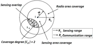
In a WSN, each sensor node has a sensing area coverage [7], [8], [9] based on its sensing range (Rs). The sensing area coverage is the region that a node can observe or monitor within its sensing range as shown in figure 1. The collective coverage of all the SENSing nodes, called as network coverage [7], [8], [9] in WSN. Similarly, each sensor node has a radio coverage [7], [8], [9] based on its communication range (Rc). The radio coverage bounded by Rc, is the region or area within which an SENSing sensor node can communicate with at least one other sensor node. Sensing coverage ensures the event monitoring within the sensing area while radio coverage [7], [8], [9] ensures error free data transmission within communication range of WSN as shown in figure 1. The sensor nodes in a WSN may be deployed such that multiple nodes can monitor an area. Thus, coverage degree (k) refers to multiple sensor nodes monitor common sensing area. K = n means n sensors are actively monitoring an area.
Fig. 1. Sensing and communication range of node
Most of the existing work [10], [11], [12], [13], [14], for energy efficient coverage, obtained by node scheduling, do not consider the residual energy of the nodes. For example, PEAS [10] is used to maximize network coverage and connectivity by maintaining adequate number of active nodes within the network field.. However, in PEAS, the wake-up rate is randomized within the desired value based on application requirement. Due to this, sleeping nodes unnecessary enter into
probing and waking mode. Therefore, the energy consumption increases and network lifetime decreases in PEAS. Random Backoff Sleep Protocol(RBSP)[15], based on backoff mechanism used for medium access in data link layer. RBSP utilizes the residual energy of the active nodes for determining the sleeping time of neighbor nodes using a dynamic sleeping window. Based on residual energy level and its associated sleeping window active node can computes the scheduling of neighbor sleeping nodes. In RBSP, the neighbor sleeping nodes wakeup very frequently when the residual energy of the current SENSing node is very less. In order to avoid this, unnecessary frequent wake-ups of sleeping nodes, at lower residual energy level, we propose Coverage Computation Based Polynomial Regression Node Scheduling (CABR) algorithm.
CABR mechanism is divided into two phases. First phase performs, Coverage Redundancy Test and second phase determines the Backoff Sleep Time (BST) using Polynomial Regression fitted for battery discharge curve. We have used the actual battery discharge pattern to computes the sleeping time duration or BST of sleeping nodes. The battery discharge curve is based on data sheet [16]. CABR uses this battery discharge curve, which is mapped with residual energy level of current ACTIVE node. Due to coverage computation test and polynomial regression, the neighbor sleeping nodes wake-up only at required instant of time or close to the death of current ACTIVE node. This leads to lesser energy consumption and increased network lifetime in CABR as compared to RBSP and PEAS. The rest of the paper is organized as follows: In section II, we review some energy efficient coverage protocols used in wireless sensor networks. We explained the computation of Coverage Computation Test and Backoff Sleep Time (BST) using battery discharge curve in section III. Section IV describes performance evaluation using simulations. Finally, we conclude our paper in section V.
2 RELATED WORK
to this, DCCA could lead to energy wastage which reduces network lifetime. Nam-Tuan et al. have presented CESS[17] protocol for energy efficient area coverage. CESS determines redundant WORKING nodes similar to DCCA [12] while maintaining sufficient coverage in the network. However, CESS provides full coverage in case of dense deployment. At the same time, there is the possibility of coverage redundancy due to coverage calculation test.
Jiguo Yu et al. have presented CTCk[13] for energy efficient coverage and connectivity in heterogeneous wireless sensor networks. CTCk is further classified as Centralized Connected Target k-Coverage algorithm (CCTCk) and Distributed Connected Target k-Coverage algorithm (DCTCk). In CCTCk and DCTCk the neighboring relay node can be used for connectivity. However, for monitoring k-coverage, multiple ACTIVE sensor nodes along with relay nodes for connectivity may increase energy consumption and reduced network lifetime. In CTCk, if the central entity (sink node) fails, it can cause a communication gap within the network.
Nam et al. have proposed a BECG [18] for energy balanced coverage within the network. In BECG protocol, the periodical node scheduling is used to exchange the node duties with neighboring sleeping nodes and vice-versa. The coverage void could be avoided however, there is possibility of coverage redundancy due to higher count of working nodes. Xink et al. presented the ECDC [14] protocol. ECDC handles the sensing area/point coverage for computation of redundant node. ECDC protocol uses randomized rotation of cluster head within the clusters for each round. In ECDC, the cluster heads are elected based on random probabilities without considering the residual energy. Due to this, ECDC does not maintained energy balanced within the network.
Mishra et al. have proposed a mechanism for monitoring the Area of Interest (AoI) [19] in the network. AoI maintains the sufficient count of active nodes in the subset. The division of network field create subsets within which set of active nodes can monitored the area of interest. Therefore, there is a possibility of incomplete coverage or coverage void in the network. Thus, full coverage, over the entire network, may not be maintained by subset. In addition, communication between multiple subsets may leads to energy consumption.
RBSP [15] is a location unaware, residual energy based distributed protocol. The random node scheduling is used in RBSP. The node scheduling mechanism is based on sleeping window which is associated with current active
node’s residual energy levels. The neighboring sleeping nodes wake-up frequently when the residual energy of the current ACTIVE node is very low. This random and frequent wake-up of a sleeping node, causes energy wastage and reduces the network lifetime. Akhlaq et al. have presented an integrated and energy-efficient protocol for Coverage, Connectivity and Communication (C3) [20]. C3 protocol is based on triangular tessellation which identify the neighbor active nodes at required position for full coverage. However, C3 does not guarantee full area coverage due to unavailability of nodes at required position (triangular tessellation). Further, the death of cluster heads could cause connectivity and communication gap in the network.
Kijun et al.[21] have proposed MAC protocol, based on a backoff algorithm, for wireless sensor networks. It used dynamic contention period based on residual energy at each node. In case of reference [21] the residual energy is considered for medium access and not for planning the coverage. In Discharge Curve Backoff Sleep Protocol (DCBSP) [22], the battery curve is used to determine the sleep time. However, the battery curve is segmented and interpolation is used. This increases the possibility of inaccurate sleep time estimates.
3 PRELIMINARIES AND ASSUMPTIONS
In this section, we describe different sensing models, which are widely used in WSNs based on application requirements [23], [24], [25]. The sensing ability of a sensor node decreases as the distance from a point of interest increases. Due to this, node can only sense a certain amount of area within the network. Thus, the sensing models can be classified as deterministic or probabilistic in nature. These sensing models have an impact on sensing area coverage, active node count and coverage lifetime within the WSN. Once the sensor nodes are deployed in the field, an algorithm is used to determine whether sufficient coverage exists in the network. Centralized or distributed algorithms could be used for this purpose. The centralized algorithms have a central entity which performs all network-related operations. However, the central entity is a single point of failure. In the cluster based algorithm, the transmission from cluster heads farther away from the base station, as well as communication between multiple cluster heads, requires higher power than single hop
communication. This increased energy
network. A distributed algorithm on another hand is run on each node within the network. In this algorithm, each node has the capability to decide its working mode with the help of neighboring ACTIVE nodes’ information. compared to centralized algorithms, distributed algorithms would tend to have uniform energy consumption which would lead to increased network lifetime and coverage. In this paper, we have design and proposed a distributed mechanism for energy efficient coverage in wireless sensor networks.
3.1 Assumption
We state our assumptions before describing the Coverage Computation Based Polynomial Regression Node Scheduling (CABR) mechanism. The communication range (Rc) is twice of sensing range (Rs). Here, Rs is the sensing range as shown in figure 1. We have used Deterministic Sensing Model, here node can sense the target upto Rs only. The sensor nodes can determine their location information using localization techniques [26]. Polynomial regression is used for discharge curve line of fit. In this battery discharge curve does not generally pass through all data points values. This may not be the correct measure which may create the measuring error between the regression predictions of a data values. However, we have tried to fit the best degree (5) of polynomial where standard error = 6:36 for 95% confidence level and correlation coefficient is (r) = 0:97.
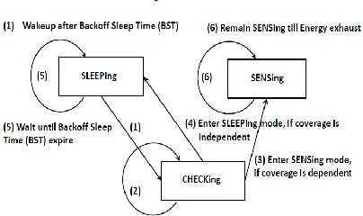
3.2 State transition of CABR
Fig. 2. State transition of CABR
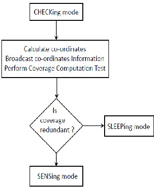
Each node in CABR works in three operating modes similar to RBSP [15]. However, we have modified the initial node scheduling as compared to RBSP. CABR has SLEEPing, CHECKing and SENSing modes and the state transition diagram for all three modes is shown in figure 2. In SLEEPing mode, a node turns its transceiver off to conserve energy. Each node in CHECKing mode broadcasts coordinates information within its communication range Rc, where Rc is the maximum radio range. The SENSing node continuously senses the physical environment for event detection and communicates with neighboring sensor nodes. In CABR, nodes are initially in the CHECking mode. By using localization techniques, all nodes can determine their location information based on distance estimation with the help of reference coordinates. After the nodes exchange their location coordinates, each node performs coverage computation test for their coverage contribution within the sensing area by identifying their neighboring nodes. If its coverage is independent (not required) of its neighbor sensor nodes, it will broadcast redundant messages to inform the neighboring nodes and enters into SLEEPing mode. Else, the node enters into SENSing mode for sensing and monitoring the field.
Fig. 3. Initial operation of CABR
3.3 Details of coverage computation test
Fig. 4. Coverage computation based on DCCA [12]
The coverage computation test of CABR is similar to DCCA [12]. CABR, uses the node coordinate (x and y) information to identify redundant sensor nodes. The coverage computation test consist of perimeter, center and distance measurement which is applied to neighboring nodes. The computation of coverage test can be explained with the help of a suitable example. Figure 4 (a) shows the coverage computation test to identify redundant nodes. There are five nodes (1,2,3,4,5), node 1 is redundant node as it is coverage by its neighbor active nodes (2,3,4,5). Therefore, node 1 can goes to SLEEPing state for the duration of Backoff Sleep Time (BST). The computation of BST is explained in the next section.
The details of coverage computation test is explained with the help of an example as follows: A node 1 uses the perimeter-test to check whether its entire perimeter is covered by other neighboring nodes. Figure 4 (b) shows, the node 1 perimeter is covered by neighbor nodes (2,3,4,5). However, the center area of node 1 is not covered by any of its neighbor nodes. Therefore, the center test determines whether the center of node 1 is covered by at least one of its perimeter neighbor node. Hence, figure 4 (c) shows, based on center test node 3 covers the center of node 1. This center test ensures that the entire sensing area of node 1 is coverage by its neighboring nodes (2,3,4,5). Finally, the distance-test, ensures that the there is no uncovered area or coverage void inside the sensing region of node 1. Hence, the distance-test as shown in figure 4 (d), must satisfy the condition: d(3; n) < d(3; 1) + Rs where n is 2, 4, 5 [12]. In this way, CABR determines the redundant nodes in order to maintained the sufficient count of SENSing nodes in the network. Further, the redundant node enters into SLEEPing state for the time duration of Backoff Sleep Time using polynomial regression on battery discharge curve. In the next section, we discussed the computation of BST.
Fig. 5. Battery discharge curve pattern [27]
3.4 Computation of Backoff Sleep Time(BST)
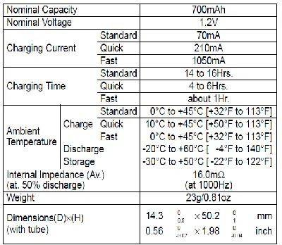
Fig. 6. Battery discharge curve of N-700AAC [16]
The technical data sheet of battery N-700AAC is shown in figure 7. To determine an accurate fit to the battery discharge curve, we first determine 10 data points from the data sheet of the battery discharge curve. The Y axis of battery discharge curve represents the nominal voltage or cell voltage whereas X axis represent the discharge time of battery. Thus, we can compute the cell voltage with respect to discharge time as y= f(x). However, we have to compute the battery discharge time with respect to cell voltage, hence we have interchange the axis (x-axis as y-axis and y-axis as x-axis) so that we can compute the battery full discharge time as y =f(x). Where, x maximum nominal voltage and y is the cutoff nominal voltage of the battery at a particular residual energy level which is computed as follows: We computed the relative voltage (Vrel) in OBSP [28]. However, in OBSP we used the different discharge curve for computation of BST.
Fig. 7. Battery specification of N-700AAC
VNominal = (1:3v - 0:9v)* (b%/100) + 0:9v ….. (1) Here, b is the battery level (Residual Energy) of node in percentage. VNominal is the nominal battery voltage. 1.3V is the maximum operating
voltage, we called this as maximum nominal voltage (VNmax) and 0.9v is cut-off voltage of battery, we called this as minimum nominal voltage VNmin is as shown in figure 6.
Fig. 8. Polynomial regression for N-700AAC
Discharge curve parameters using polynomial regression (Degree 5)
Name: Polynomial regression (Degree 5) Kind: Regression
Family: Linear Regression
Equation: y = a + bx2 + cx3 + …… No of independent variable: 1 Standard error: 6.365744
Correlation coefficient (r) = 0.9706 Coefficient of determination (r2) = 0.9421 DOF : 14
AICC: 81.89
Fig. 9. Regression analysis for standard error
coefficient of polynomial regression (degree = 5) for battery discharge curve. We have used MATLAB [29] for determining the curve fits. The Regression Analysis is used for constructing a mathematical equation of battery discharge curve. Therefore, the Backoff Sleep Time (BST) derived from Polynomial Regression for N-700AAC is shown as:
BST=a+bVNominal+cV2Nominal+dV3Nominal (2)
Here, a, b, c, d, e and f are polynomial coefficients as shown in figure 9, BST is the Backoff Sleep Time and it indicates that after BST minutes of operation, the battery will be fully discharged. In the next section, we evaluate the performance of CABR and compare it with RBSP and PEAS.
4 PERFORMANCE EVALUATIONS
We have implemented CABR, RBSP and PEAS in NS- 2 [30]. The energy model in this protocol is similar to RBSP [15] and PEAS[10], where
Sleep:Idle:Tx:Rx as
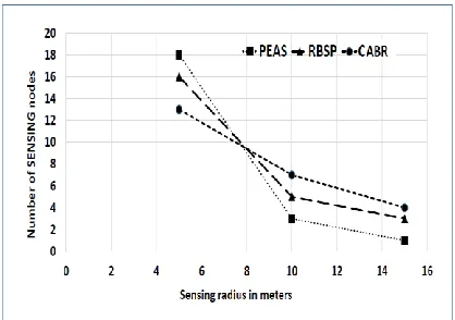
0.03mW:12mW:60mW:12mW. We assume that the maximum sensing range is 5 meters and the transmission range is twice of sensing range. The initial energy of each node is set at 1 Joules. We run the simulation for 150 sec. The packet size of HELLO and REPLY messages are 25 bytes each. We set node density as 100 nodes in the network field of 50*50m2. Nodes are randomly deployed using inbuilt random generator function in the field and nodes remain static after deployment. Figure 10 shows the number of SENSing nodes with respect to sensing range. As sensing range increases, the sensing area per node may also increases. Thus, we have varied the sensing range in meters as shown in figure 11. We can see that, the average Number of SENSing nodes in case of CABR is higher compared to RBSP and PEAS due to optimal wakeups of sleeping nodes based on coverage computation based polynomial regression for battery discharge curve.
Fig. 10. Number of SENSing nodes with respect to time
Fig. 11. Effect of sensing radius on SENSing node count
percentage in terms on number SENSing nodes present in the network for monitoring the field. The maximum network field is about 50*50meter2 and
maximum coverage area per node is about
∏(Rs)2. Therefore, we can compute the maximum number of SENSing node present in the network for monitoring an area which can be represented as coverage area as 50*50/(5)2 = 32, which indicate that at least 32 nodes are required to cover the entire network field. In figure 13, we can see the area coverage percentage for CABR for a longer as
Fig. 12. Total energy consumption wrt. Time
Fig. 13. Coverage are percentage wrt. Time
compare to RBSP and PEAS. In addition, CABR protocol provides approximately 16% and 12% of higher coverage as compared to PEAS and RBSP. Hence, CABR maintains adequate number of nodes in SENSing mode for a longer period of time as compared other protocols.
5 CONCLUSION AND FUTURE WORK
We have proposed Coverage Computation Based Polynomial Regression Node Scheduling (CABR) algorithm using battery discharge curve. CABR ensures minimal coverage redundancy by executing coverage computation test and optimal sleep time derived from polynomial regression for node
scheduling. The coverage computation test determines the adequate number of SENSing nodes while polynomial regression maintains optimal wakeup rate within the SLEEPing nodes. CABR avoid random and unnecessary frequent wake-up of sleeping node. This leads to lesser energy consumption and increased coverage and network lifetime as compared to other protocols.
Simulation results show that, CABR, RBSP and PEAS maintain adequate number of SENSing nodes for maintaining sufficient sensing area coverage. Total energy consumption of CABR is lesser compared to that of RBSP and PEAS. The total energy consumption of CABR is lesser than that of RBSP by 15% and lesser by 32% as compared to PEAS. CABR protocol provides approximately 100% sensing area coverage upto 60 seconds while RBSP and PEAS provide up to 30 and 40 seconds of network lifetime. In our future work, we will extend our protocol to handle coverage voids and maintain certain percentage of area coverage by SENSing nodes within the networks.
6 REFERENCES
[1] J. Zheng and A. Jamalipour, Wireless Sensor Networks A Networking Perspective. Hoboken, New Jersey: A JOHN WILEY and SONS, 2009.
[2] C.-Y. CHONG and S. P. KUMAR, “Sensor networks: Evolution, opportunities, and challenges,” in Proceedings of the IEEE, vol. 91, no. 8, August 2003, pp. 1247–1256. [3] V. Raghavendra, K. R., F. A., and V. G.,
“Computational intelligence in wireless sensor network: A survey,” IEEE Communication Surveys and Tutorials, vol. 13, no. 1, 2009, pp. 68–96
[4] K. Akkaya and M. Younis, “A survey on routing protocols for wireless sensor networks,” Science Direct, Ad Hoc Networks, vol. 3, 2005, pp. 325–349.
[5] [5] J. J.-N. L. Imrich Chlamtac, Marco Conti, “Mobile ad hoc networking: imperatives and challenges,” Ad Hoc Networks, vol. 1, no. 1, 2003, pp. 13–64.
[6] B. D.-P. D. Jeroen Hoebeke, Ingrid Moerman, “An overview of mobile ad hoc networks: applications and challenges,” Journal of the Communications Network, vol. 3, no. 3, Sep. 2004, pp. 60–66.
[8] A. I. F., S. W, S. Y, and C. E., “Wireless sensor networks: A survey,” Elsevier, Computer Networks, vol. 38, no. 4, march 2002, pp. 393–422.
[9] G. Amit and D. Sajal, “Coverage and connectivity issues in wireless sensor networks: A survey,” Science Direct, Pervasive and Mobile Computing, vol. 4, 2008, pp. 303– 334.
[10]Y. Fan, Z. Gary, C. Jesse, L. Sungwu, and Z. Lixia, “Peas: A robust energy conserving protocol for long-lived sensor networks,” 23rd International Conference on Distributed Computing Systems (DCS’ 02), May 2002, pp.28–37.
[11]G. Chao and M. Prasant, “Power conservation and quality of surveillance in traget tracking sensor networks,” in Proceedings of 10th Annual International Conference on Mobile Computing and Networking (ACM MobiCom’ 04), Pennsylvania, USA, Sep. 2004, pp. 129– 143.
[12]T. Nurcan and W. Wenye, “Effective coverage and connectivity preserving in wireless sensor networks,” in IEEE WCNC, March 2007, p. 3388 -3393.
[13]J. Jiguo Yu, Y. Chen, L. Ma, B. Huang, and X. Cheng, “On connected target k-coverage in heterogeneous wireless sensor networks,” Sensors Journal, vol. 16, no. 104, January 2016, pp. 1–21.
[14]G. Xin, Y. Jiguo, Y. Dongxiao, W. Guanghui, and L. Yuhua, “Ecdc: An energy and coverage-aware distributed clustering protocol for wireless sensor networks,” Computer and Electrical Engineering, Elsevier, vol. 40, September 2014, pp. 384–398.
[15]M. Avinash and R. Vijay, “Random backoff sleep protocol for energy efficient coverage in wireless sensor networks.” Smart Innovation, System and Technology, Springer, Varlag, vol. 28, no. 2, May 2014, pp. 323–331.
[16]“N-700AAC data sheet - sanyo inc,” Cadnica. [17] L. Nam-Tuan and J. Y. Min, “Energy-efficient
coverage guarantees scheduling and routing strategy for wireless sensor networks,” International Journal of Distributed Sensor Networks, vol. 2015, May 2015, pp. 1–12. [18] N. Le, N. Saha, R. Mondal, S. Chae, and Y.
Jang, “Balanced energy and coverage guaranteed protocol for wireless sensor networks,” International Conference on Electrical Information and Communication Technology (EICT), Feb. 2013.
[19] M. Sudip, M. P. Kumar, and M. S. Obaidat, “Connectivity preserving localized coverage
algorithm for area monitoring using wireless sensor networks,” Computer Communication, Elsevier, vol. 34, no. 00, March 2011, pp. 1484–1496,.
[20] A. Muhammad, S. T. R., and S. E. M., “C3: an energy-efficient protocol for coverage, connectivity and communication in wsn’s,” Pers Ubiquit Computing, Springer-Verlag., vol. 18, November 2014, pp. 1117–1133,.
[21] C. Chiwoo, P. Jinsuk, K. Jinnyun, L. Icksoo, and H. Kijun, “A random backoff algorithm for wireless sensor networks.” Next Generation Telegraphic and wired/wireless Advanced Networking,LNCS, Springer, vol. 4003, no. 5, Sep. 2006, pp. 108–117,.
[22] A. More and V. Raisinghani, “Discharge cuve backoff sleep protocol for energy efficient coverage in wireless sensor networks,” in Procedia computer science, Elsevier, vol. 57, Sep. 2015, pp. 1131–1139.
[23]S. C. Ashraf Hossain and P. Biswas, “Impact of sensing model on wireless sensor network coverage,” IET Wireless Sensor Systems, vol. 2, no. 3, January 2012, pp. 272–281.
[24] S. Kumar and D. K. Lobiyal, “Sensing coverage prediction for wireless sensor networks in shadowed and multipath environment,” The Scientific World Journal, Hindawi Publishing Corporation, vol. 2013, , September 2013, pp. 1–11.
[25] S. Bhowmik and C. Giri, “A novel fuzzy sensing model for sensor nodes in wireless sensor network,” Advances in Intelligent Systems and Computing, vol. 182, no. 3, August 2013, pp. 365–371.
[26]S. J. A., “Radiometry and friis transmission equation,” American journal of physics, vol. 81, no. 1, Jan. 2013, pp. 1–33,.
[27]M. Crompton., Battery Reference Book. Linacre House, Jordan Hill, Oxford OX2 8DP 225 Wildwood Avenue, Woburn, MA 01801-2041: Reed educational and professional publishing ltd, 2000.
[28]M. Avinash and sharad wagh, “Energy efficient coverage using optimized node scheduling in wireless sensor networks,” 1st International Conference on Next Generation Computing Technologies (NGCT), Sep. 2015, pp. 291 – 295,.
[29] MATLAB-2013b, “Matlab simulink,” http://www.mathworks.com/matlab, 2013, [Online; accessed 21-Aug-2014].
[30]Ns 2, “Network simulator,”