http://wrap.warwick.ac.uk
Original citation:
Ogden, Helen E.. (2015) A sequential reduction method for inference in generalized
linear mixed models. Electronic Journal of Statistics, Volume 9 . pp. 135-152.
Permanent WRAP url:
http://wrap.warwick.ac.uk/66254
Copyright and reuse:
The Warwick Research Archive Portal (WRAP) makes this work of researchers of the
University of Warwick available open access under the following conditions.
This article is made available under the Creative Commons Attribution 2.5 Generic (CC
BY 2.5) license and may be reused according to the conditions of the license. For more
details see:
http://creativecommons.org/licenses/by/2.5/
A note on versions:
The version presented in WRAP is the published version, or, version of record, and may
be cited as it appears here.
Vol. 9 (2015) 135–152 ISSN: 1935-7524 DOI:10.1214/15-EJS991
A sequential reduction method for
inference in generalized linear mixed
models
Helen E. Ogden
Department of Statistics, University of Warwick Coventry, CV4 7AL, United Kingdom
e-mail:[email protected]; url:warwick.ac.uk/heogden
Abstract: The likelihood for the parameters of a generalized linear mixed model involves an integral which may be of very high dimension. Because of this intractability, many approximations to the likelihood have been pro-posed, but all can fail when the model is sparse, in that there is only a small amount of information available on each random effect. The sequential re-duction method described in this paper exploits the dependence structure of the posterior distribution of the random effects to reduce substantially the cost of finding an accurate approximation to the likelihood in models with sparse structure.
MSC 2010 subject classifications:Primary 62F10; secondary 62J15. Keywords and phrases:Graphical model, intractable likelihood, Laplace approximation, pairwise comparison, sparse grid interpolation.
Received August 2014.
Contents
1 Introduction . . . 136
2 The generalized linear mixed model . . . 136
2.1 The model . . . 136
2.2 Example: Pairwise competition models . . . 137
2.3 The likelihood . . . 137
2.4 Existing approximations to the likelihood . . . 138
2.5 Bayesian inference . . . 139
3 The sequential reduction method . . . 139
3.1 Conditional independence structure . . . 139
3.2 Exploiting the clique factorization . . . 140
3.3 The sequential reduction method . . . 141
3.4 A specific clique factorization . . . 142
3.5 Approximate function representation . . . 142
3.6 Computational complexity . . . 145
3.7 An R package for sequential reduction . . . 146
4 Examples . . . 146
4.1 Tree tournament . . . 146
4.2 An animal behavior “tournament”: Augrabies Flat lizards . . . . 148
4.3 A three-level model . . . 149
5 Conclusions . . . 150
Acknowledgements . . . 150
Supplementary Material . . . 150
References . . . 151
1. Introduction
Generalized linear mixed models are a natural and widely used class of models, but one in which the likelihood often involves an integral of very high dimension. Because of this intractability, many alternative methods have been developed for inference in these models.
One class of approaches involves replacing the likelihood with some approxi-mation, for example using Laplace’s method or importance sampling. However, these approximations can fail in cases where the structure of the model is sparse, in that only a small amount of information is available on each random effect, especially when the data are binary.
The likelihood may be written as an integral over the random effects. If there are a large number of random effects, then it will be computationally infeasible to obtain an accurate approximation to this integral by direct numerical inte-gration. However, it is not always necessary to compute this high-dimensional integral to find the likelihood. In a two-level random intercept model, indepen-dence between clusters may be exploited to write the likelihood as a product of one-dimensional integrals, so it is relatively easy to obtain a good approxi-mation to the likelihood, even if there are large number of random effects. In more complicated situations it is often not immediately obvious whether any such simplification exists.
The ‘sequential reduction’ method developed in this paper exploits the struc-ture of the integrand to simplify computation of the likelihood, and as a result allows a fast and accurate approximation to the likelihood to be found in many cases where existing approximation methods fail. Examples are given to demon-strate the new method, including pairwise competition models and a model with nested structure.
2. The generalized linear mixed model
2.1. The model
A generalized linear mixed model allows the distribution of a response Y = (Y1, . . . , Ym) to depend on observed covariates through a linear predictor η. Conditional onη, the distribution ofY is assumed to have exponential family form, with meanµ=E(Y|η) =g−1(η), for some known link functiong(.). We model
where β = (β1, . . . , βp) are fixed effects, with fixed design matrixX, andu= (u1, . . . , un) are random effects, with design matrix Z(ψ) whose entries may depend on a parameter ψ. We assume that the ui are independent standard normal variables. At first sight, this assumption of independent and identically distributed random effects appears restrictive, but by suitable choice of Z(ψ), we may let Z(ψ)uhave any multivariate normal distribution with mean zero, to coincide with the standard parameterization of a generalized linear mixed model (as in Breslow and Clayton,1993, for example).
For each item i, we define the ‘active’ set Ai={j :Zji(ψ)6= 0}to describe which components of the response involve the random effectui. We will say the generalized linear mixed model has ‘sparse structure’ if this active set is small for most items. These sparse models are particularly problematic for inference, especially when the data are binary, because the amount of information available on each random effect is small.
2.2. Example: Pairwise competition models
Consider a tournament among n players, consisting of contests between pairs of players. For each contest, we observe a binary outcome: either i beats j
or j beats i. We suppose that each player i has some ability λi, and that conditional on all the abilities, the outcomes of the contests are independent, with distribution depending on the difference in abilities of the players i and
j, so that Pr(ibeatsj|λ) = g−1(λ
i −λj) for a link function g(.) such that
g−1(−t) = 1−g−1(t). If g(.) = logit(.), then this describes a Bradley-Terry model (Bradley and Terry, 1952). If g(.) = Φ−1(.) (the probit link), then it describes a Thurstone-Mosteller model (Thurstone,1927; Mosteller,1951).
If covariate informationxi is available for each player, then interest may lie in the effect of the observed covariates on ability, rather than the individual abilitiesλi themselves. We allow the ability of playerito depend on the covari-ates xi through λi = βTxi+σui, where ui are independent N(0,1) samples. This gives a generalized linear mixed model, depending on a linear predictor
η with components ηr = λp1(r)−λp2(r), where p1(r) and p2(r) are the first
and second player involved in matchr. The active set for each player is the set of matches that player competes in, so the model will have sparse structure if each player competes in only a small number of matches, a common scenario in practice.
2.3. The likelihood
Let f(.|ηi) be the density of Yi, conditional on knowledge of the value of ηi, and writeθ= (β, ψ) for the full set of model parameters. Conditional onη, the components of Yare independent, so that
L(θ) = Z
Rn m Y
i=1
f yi|ηi=XiTβ+Zi(ψ)Tu n Y
j=1
where Xi is the ith row of X, and Zi(ψ) is the ith row of Z(ψ). Unless n is very small, it will not be possible to approximate the likelihood well by direct computation of thisn-dimensional integral.
2.4. Existing approximations to the likelihood
Pinheiro and Bates (1995) suggest using a Laplace approximation to the inte-gral (1). Write
g(u1, . . . , un|y, θ) = m Y
i=1
f yi|ηi=XiTβ+Zi(ψ)Tu n Y
j=1
φ(uj)
for the integrand of the likelihood. This may be thought of as a non-normalized version of the posterior density foru, givenyandθ. For each fixedθ, the Laplace approximation relies on a normal approximation to this posterior density. To find this normal approximation, letµθmaximize logg(u|y, θ) overu, and write Σθ = −Hθ−1, where Hθ is the Hessian resulting from this optimization. The normal approximation tog(.|y, θ) will be proportional to aNn(µθ,Σθ) density. Writinggna(.|y, θ) for the normal approximation tog(.|y, θ),
gna(u|y, θ) = g(µθ|y, θ)
φn(µθ;µθ,Σθ)
φn(u;µθ,Σθ),
where we writeφn(.;µ,Σ) for theNn(µ,Σ) density. When we integrate overu, only the normalizing constant remains, so that
LLaplace(θ) = g(µθ|y, θ)
φn(µθ;µθ,Σθ)
= (2π)−n2(det Σθ)−12g(µθ|y, θ).
In the case of a linear mixed model, the approximating normal density is precise, and there is no error in the Laplace approximation to the likelihood. In other cases, and particularly when the response is discrete and may only take a few values, the error in the Laplace approximation may be large. In the case that n is fixed, and m → ∞, the relative error in the Laplace approximation may be shown to tend to zero. However, in the type of model we consider here,
In cases where the Laplace approximation fails, Pinheiro and Bates (1995) suggest constructing an importance sampling approximation to the likelihood, based on samples from the normal distribution Nn(µθ,Σθ). Writing
w(u;θ) = g(u|y, θ)
φn(u;µθ,Σθ)
,
the likelihood may be approximated by LIS(θ) = PN
i=1w(u(i);θ)/N, where u(i)∼N(µθ,Σθ).
Unfortunately, there is no guarantee that the variance of the importance weights w(u(i);θ) will be finite. In such a situation, the importance sampling approximation will still converge to the true likelihood as N → ∞, but the convergence may be slow and erratic, and estimates of the variance of the ap-proximation may be unreliable.
2.5. Bayesian inference
From a Bayesian perspective, Markov chain Monte Carlo methods could be used to sample from the posterior distribution. However, such methods are compu-tationally intensive, and it can be difficult to detect whether the Markov chain has converged to the correct distribution. Rue, Martino and Chopin (2009) sug-gest the Integrated Nested Laplace Approximation (INLA) to approximate the marginal posterior distribution of each parameter. INLA is computationally ef-ficient, but Fong, Rue and Wakefield (2010) note that the approximation may perform poorly in models for binary data. In situations where the Laplace ap-proximation to the likelihood fails, INLA may be also unreliable.
We do not consider these methods further, and instead focus on those meth-ods which provide a direct approximation to the marginal likelihood (1).
3. The sequential reduction method
3.1. Conditional independence structure
We now consider the distribution of the unknown random effectsugiveny, at fixed parameter valueθ, which has density proportional to the integrand of the likelihood g(u|y, θ). We will refer to this distribution as the posterior distribu-tion ofugivenyandθ. Despite this terminology, our aim is to approximate the likelihood, which is the normalizing constant associated with this distribution, rather than to conduct Bayesian inference.
Recall that for each item i we define the active set Ai to be the indices of the non-zero components of the ith column ofZ(ψ). If the active sets Ai and
Aj are disjoint, ui and uj will be conditionally independent in the posterior distribution, given the values of all the other random effects.
1. A vertex for each random effect
2. An edge between two verticesiandj ifAi∩Aj6=∅.
If there is no edge betweeniandjinG,uiandujare conditionally independent in the posterior distribution, given the values of all the other random effects, so the posterior distribution of the random effects has the pairwise Markov property with respect to G. We call G the posterior dependence graph for u giveny.
In a pairwise competition model, the posterior dependence graph simply con-sists of a vertex for each player, with an edge between two vertices if those players compete in at least one contest. For models in which each observation relies on more than two random effects, an observation will not be represented by a single edge in the graph.
The problem of computing the likelihood has now been transformed to that of finding a normalizing constant of a density associated with an undirected graphical model. In order to see how the conditional dependence structure can be used to enable a simplification of the likelihood, we first need a few definitions. A complete graph is one in which there is an edge from each vertex to every other vertex. A clique of a graphG is a complete subgraph of G, and a clique is said to be maximal if it is not itself contained within a larger clique. For any graphG, the set of all maximal cliques ofG is unique, and we write M(G) for this set.
The Hammersley-Clifford theorem (Besag,1974) implies thatg(.|y, θ) factor-izes over the maximal cliques ofG, so that we may write
g(u|y, θ) = Y C∈M(G)
gC(uC)
for some functions gC(.). A condition needed to obtain this result using the Hammersley-Clifford theorem is that g(u|y, θ) > 0 for all u. This will hold in this case because φ(ui) > 0 for all ui. In fact, we may show that such a factorization exists directly. One particular such factorization is constructed in Section 3.4, and would be valid even if we assumed a random effects density
fu(.) such thatfu(ui) = 0 for someui.
3.2. Exploiting the clique factorization
Jordan (2004) reviews some methods to find the marginals of a density factorized over the maximal cliques of a graph. While these methods are well known, their use is typically limited to certain special classes of distribution, such as discrete or Gaussian distributions. We will use the same ideas, combined with a method for approximate storage of functions, to approximate the marginals of the distribution with density proportional tog(.|y, θ), and so approximate the likelihoodL(θ) =R
Rng(u|y, θ)du.
factorization of g(.|y, θ) over the maximal cliques of the posterior dependence graph of {u1, . . . , un}, and the idea will be to write the marginal posterior density of{u2, . . . , un}as a product over the maximal cliques of a new marginal posterior dependence graph. Once this is done, the process may be repeated n
times to find the likelihood. We will writeGifor the posterior dependence graph of {ui, . . . , un}, so we start with posterior dependence graph G1 = G. Write
Mi=M(Gi) for the maximal cliques of Gi.
Factorizingg(.|y, θ) over the maximal cliques ofG1 gives
g(u|y, θ) = Y C∈M1
g1C(uC),
for some functions {g1C(.) :C∈M1}. To integrate overu1, it is only necessary to integrate over maximal cliques containing vertex 1, leaving the functions on other cliques unchanged. Let N1 be the set of neighbors of vertex 1 in G (including vertex 1 itself). Then
Z
g(u|y, θ)du1= Z
Y
C∈M1:C⊆N1
gC1(uC)du1 Y
˜
C∈M1: ˜C6⊆N1
g1C˜(uC˜)
= Z
g1N1(u1,uN1\1)du1 Y
˜
C∈M1: ˜C6⊆N1
gC1˜(uC˜).
Thus g1
N1(.) is obtained by multiplication of all the functions on cliques which are subsets ofN1. This is then integrated overu1, to give
gN21\1(uN1\1) =
Z
g1N1(u1,uN1\1)du1.
The functions on all cliques ˜C which are not subsets ofN1 remain unchanged, withg2
˜
C(uC˜) =g1C˜(uC˜).
This defines a new factorization ofg(u2, . . . un|y, θ) over the maximal cliques
M2of the posterior dependence graph for{u2, . . . , un}, whereM2containsN1\1, and all the remaining cliques in M1 which are not subsets of N1. The same process may then be followed to remove eachuiin turn.
3.3. The sequential reduction method
We now give the general form of a sequential reduction method for approxi-mating the likelihood. We highlight the places where choices must be made to use this method in practice. The following sections then discuss each of these choices in detail.
1. Theui may be integrated out in any order. Section3.6 discusses how to choose a good order, with the aim of minimizing the cost of approximat-ing the likelihood. Reorder the random effects so that we integrate out
2. Factorize g(u|y, θ) over the maximal cliques M1 of the posterior depen-dence graph, as g(u|y, θ) = Q
C∈M1g1C(uC). This factorization is not unique, so we must choose one particular factorization{g1
C(.) :C∈M1}. Section 3.4gives the factorization we use in practice.
3. Once u1, . . . , ui−1 have been integrated out (using some approximate method), we have the factorization ˜g(ui, . . . , un|y, θ) = QC∈MigCi(uC), of the (approximated) non-normalized posterior for ui, . . . , un. Write
gNi(uNi) = Y
C∈Mi:C⊂Ni
gCi (uC).
We then integrate overui(using a quadrature rule), and store an approx-imate representation ˜gNi\i(.) of the resulting functiongNi\i(.). In Section 3.5we discuss the construction of this approximate representation. 4. Write
˜
g(ui+1, . . . , un|y, θ) = ˜gNi\i(uNi\i) Y
C∈Mi:C6⊂Ni
giC(uC),
defining a factorization of the (approximated) non-normalized posterior density of {ui+1, . . . , un}over the maximal cliques Mi+1 of the new pos-terior dependence graphGi+1.
5. Repeat steps (3) and (4) fori= 1, . . . , n−1, then integrate ˜g(un|y, θ) over
un to give the approximation to the likelihood.
3.4. A specific clique factorization
The general method described in Section3.3is valid for an arbitrary factoriza-tion ofg(u|y, θ) over the maximal cliquesM1of the posterior dependence graph. To use the method in practice, we must first define the factorization used.
Given an ordering of the vertices, order the cliques in M1 lexicographically according to the set of vertices contained within them. The observation vector y is partitioned over the cliques inM1 by including inyC all the observations only involving items in the cliqueC, which have not already been included in yB for some earlier clique in the ordering,B. Writea(C) for the set of vertices appearing for the first time in cliqueC. Let
g1
C(uC) =f(yC|uC) Y
j∈a(C)
φ(uj).
Theng(u|y) =Q C∈M1g
1
C(uC), sogC1(.) does define a factorization ofg(.|y).
3.5. Approximate function representation
3.5.1. A modified function for storage
evaluate gNi\i(.), and a method of interpolation between those points, which will be used later in the algorithm if we need to evaluate gNi\i(uNi\i) for some
uNi\i6∈Si.
We would like to minimize the size of the absolute error in the interpolation for those points uNi\i at which we will later interpolate. The quality of the interpolation may be far more important at some pointsuNi\i than at others. We will transform to a new function rNi\i(uNi\i) = gNi\i(uNi\i)hNi\i(uNi\i), where we choose hNi\i(.) so that the size of the absolute interpolation error for
rNi\i(.) is of roughly equal concern across the whole space. Given an interpo-lation method for rNi\i(.), we obtain interpolated values for gNi\i(.) through
ginterpN
i\i (uNi\i) =r
interp
Ni\i (uNi\i)/hNi\i(uNi\i), so we must ensure that hNi\i(.) is easy to compute.
Recall that we may think of the original integrand g(.|y, θ) as being the non-normalized posterior density foru|y, θ. The region where where we will in-terpolate a large number of points corresponds to the region where the marginal posterior density ofuNi\i|y, θis large. Ideally, we would choosehNi\i(.) to make
rNi\i(.) proportional to the density ofuNi\i|y, θ, but this density is difficult to compute.
To solve this problem, we make use of the normal approximation tog(.|y, θ) used to construct the Laplace approximation to the likelihood, which approx-imations the posterior distribution u|y, θ as Nn(µ,Σ). The marginal posterior distribution of uNi\i|y, θ may therefore be approximated as Nd(µNi\i,ΣNi\i), whered=|Ni\i|. We choosehNi\i(.) to ensure that the normal approximation to rNi\i(.) (computed as described in Section 2.4) is Nd(µNi\i,ΣNi\i). That is, we choose loghNi\i(.) to be a quadratic function, with coefficients chosen so that ∇loghNi\i(µNi\i) = −∇loggNi\i(µNi\i) and ∇
T∇logh
Ni\i(µNi\i) = −Σ−1N
i\i− ∇
T∇logg
Ni\i(µNi\i).
3.5.2. Storing a function with a normal approximation
Suppose that f(.) is a non-negative function on Rd, for which we want to store an approximate representation, and that we may approximate f(.) with
fna(x) ∝ φ
d(x, µ,Σ), for some µ and Σ. In our case, the function f(.) which we store isrNi\i(.), of dimension d=|Ni\i|, and with normal approximation
Nd(µNi\i,ΣNi\i).
We transform to a new basis. Letz=A−1(x−µ), whereAis chosen so that
AAT = Σ. More specifically, we choose A =P D, where P is a matrix whose columns are the normalized eigenvectors of Σ andDis a diagonal matrix with di-agonal entries the square roots of the eigenvalues of Σ. Writefz(z) =f(Az+µ), and letc(z) = logfz(z)−logφd(z,0, I), so thatc(.) will be constant if the normal approximation is precise. We storec(.) by evaluating at some fixed points forz, and specifying the method of interpolation between them. The choice of these points and the interpolation method is discussed in the next section. Given the interpolation method for c(.), we may definefinterp(x) = exp{cinterp(A−1(x−
If g(u|y, θ)∝φn(u, µ,Σ), there will be no error in the Laplace approxima-tion to the likelihood. In this situaapproxima-tion,c(.) will be constant, and the sequential reduction approximation will also be exact. In situations where the normal ap-proximation is imprecise,c(.) will no longer be constant, and we may improve on the baseline (Laplace) approximation to the likelihood by increasing the number of points used for storage.
3.5.3. Sparse grid interpolation
In order to store an approximate representation of the standardized modifier function c(.), we will compute values of c(.) at a fixed set of evaluation points, and specify a method of interpolation between these points. We now give a brief overview of the interpolation methods based on sparse grids of evaluation points. Some of the notation we use is taken from Barthelmann, Novak and Ritter (2000), although there are some differences: notably that we assumec(.) to be a function on Rd, rather than on the d-dimensional hypercube [−1,1]d, and we will use cubic splines, rather than (global) polynomials for interpola-tion.
First we consider a method for interpolation for a one-dimensional function
c:R→R. We evaluatec(.) atmlpointss1, . . . , sml and write
Ul(c) = ml X
j=1
c(sj)alj,
where theal
j are basis functions. The approximate interpolated value ofc(.) at any pointxis then given byUl(c)(x).
Here l denotes the level of approximation, and we suppose that the set of evaluation points is nested so that at levell, we simply use the first ml points of a fixed set of evaluation pointsS={s1, s2, . . .}.We assume thatm1= 1, so at the first level of approximation, only one point is used, andml = 2l−1 for
l > 1, so there is an approximate doubling of the number of points when the level of approximation is increased by one.
The full grid method of interpolation is to take mlj points in dimensionj, and compute at each possible combination of those points. We write
(U1⊗ · · · ⊗ Ud)(c) = ml1 X
j1=1
. . .
mld X
jd=1
c(sj1, . . . , sjd)
al1
j1⊗ · · · ⊗a
ld jd
,
where
(al1
j1⊗ · · · ⊗a
ld
jd)(x1, . . . , xd) =a l1
j1(x1)× · · · ×a
ld jd(xd). Thus, in the full grid method, we must evaluatec(.) atQd
j=1mlj =O(
Qd
j=12lj) =
O(2Plj) points. This will not be possible ifPd
In order to construct an approximate representation of c(.) in reasonable time, we could limit the sumPd
j=1lj used in a full grid to be at mostd+k, for somek≥0. If k >0, there are many possibilities for ‘small full grids’ indexed by the levelsl= (l1, . . . , ld) which satisfy this constraint. A natural question is how to combine the information given by each of these small full grids to give a good representation overall.
For a univariate functionc(.), let
∆l(c) =Ul(c)− Ul−1(c) = ml−1
X
j=1
c(sj) h
ajl−ajl−1i+ ml X
j=ml−1+1
c(sj)ajl,
forl >1, and ∆1=U1. Then ∆l gives the quantity we should add the approx-imate storage of c(.) at levell−1 to incorporate the new information given by the knots added at level l.
Returning to the multivariate case, the sparse grid interpolation of c(.) at levelk is given by
cinterpk = X
l:|l|≤d+k
(∆l1⊗ · · · ⊗∆ld)(c).
To store c(.) on a sparse grid at level k, we must evaluate at O(dk+1) points, which allows approximate storage for much larger dimension dthan is possible using a full grid method.
Barthelmann, Novak and Ritter (2000) use global polynomial interpolation for a function defined on a hypercube, with the Chebyshev knots. We prefer to use cubic splines for interpolation, since the positioning of the knots is less critical. Since we have already standardized the function we wish to store, we use the same knots in each direction, and choose these standard knotsslat level
lto bemlequally spaced quantiles of aN(0, τk2) distribution. Askincreases, we choose largerτk, so that the size of the region covered by the sparse grid increases with k. However, the rate at whichτk increases should be sufficiently slow to ensure that the distance between the knots sk decreases with k. Somewhat arbitrarily, we choose τk = 1 + k2, which appears to work reasonably well in practice.
3.5.4. Bounded interpolation
To ensure that gNi(.) remains integrable at each stage, we impose an upper boundM on the interpolated value ofc(.). In practice, we chooseM to be the largest value ofc(z) observed at any of the evaluation points.
3.6. Computational complexity
The random effects may be removed in any order, so it makes sense to use an ordering that allows approximation of the likelihood at minimal cost. This problem may be reduced to a problem in graph theory: to find an ordering of the vertices of a graph, such that when these nodes are removed in order, joining together all neighbors of the vertex to be removed at each stage, the largest clique obtained at any stage is as small as possible. This is known as the triangulation problem, and the smallest possible value, over all possible orderings, of the largest clique obtained at some stage is known as the treewidth of the graph.
Unfortunately, algorithms available to calculate the treewidth of a graph on
n vertices can take at worst O(2n) operations, so to find the exact treewidth may be too costly for n at all large. However, there are special structures of graph which have known treewidth, and algorithms exist to find upper and lower bounds on the treewidth in reasonable time (see Bodlaender and Koster,
2008,2010). We use a constructive algorithm for finding an upper bound on the treewidth, which outputs an elimination ordering achieving that upper bound, to find a reasonably good (though not necessarily optimal) ordering.
3.7. An R package for sequential reduction
The sequential reduction method is implemented in R (R Core Team, 2014) by the package glmmsr, included as supplementary material (Ogden, 2015). The code for sparse grid interpolation is based on the efficient storage schemes suggested by Murarasu et al. (2011). Code to reproduce the examples of Section
4is also provided.
4. Examples
We give some examples to compare the performance of the proposed sequential reduction method with existing methods to approximate the likelihood. The first two examples here are of pairwise competition models (a simple tree tournament with simulated data, and a more complex, real-data example); the third is a mixed logit model with two nested layers of random effects.
4.1. Tree tournament
Consider observing a tree tournament, with structure as shown in Figure 1a. Suppose that there is a single observed covariatexi for each player, whereλi=
βxi+σuiandui∼N(0,1). We consider one particular tournament with this tree structure, simulated from the model withβ= 0.5 andσ= 1.5. We suppose that we observe two matches between each pair of competing players. The covariates
xi are independent draws from a standard normal distribution.
reduc-(a) Tree tournament (b) Lizards tournament
. . .
100 times
(c) Three-level model
[image:14.612.119.441.118.244.2]Fig 1. The posterior dependence graphs for the examples.
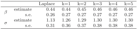
Table 1
The parameter estimates and standard errors for the tree tournament
Laplace k=1 k=2 k=3 k=4 k=5
β estimate 0.44 0.44 0.45 0.46 0.46 0.46 s.e. 0.26 0.27 0.27 0.27 0.27 0.27
σ estimate 1.13 1.26 1.29 1.30 1.30 1.30 s.e. 0.31 0.36 0.37 0.38 0.38 0.38
tion method with sparse grid storage at levelk, the cost of approximating the likelihood at each point will be O(n4k). In reality, the computation time does not quadruple each time kis increased, since the computation is dominated by fixed operations whose cost does not depend onk. To compute the approxima-tion to the likelihood at a single point took about 0.02 seconds for the Laplace approximation, 0.22 seconds fork= 1, 0.24 seconds fork= 2, 0.24 seconds for
k= 3, 0.27 seconds fork= 4 and 0.30 seconds fork= 5.
Table1gives the estimates ofβ andσresulting from each approximation to the likelihood. The estimates ofβ are similar for all the approximations, but the estimate ofσfound by maximizing the Laplace approximation to the likelihood is smaller than the true maximum likelihood estimator.
[image:14.612.159.398.301.352.2]1 10 100 1000 10000
1.0
1.2
1.4
1.6
1.8
2.0
Time (seconds)
D
iff
er
en
ce
in
L
og
lik
elih
o
o
d
s
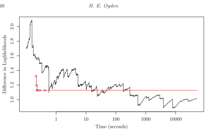
Fig 2. Importance sampling and sequential reduction approximations to ℓ(0.46,1.30)− ℓ(0.60,2.00), plotted against the time taken to find the approximation, on a log scale. The sequential reduction approximation converges in less than a second, but the importance sam-pling approximation has still not converged after over 14 hours.
4.2. An animal behavior “tournament”: Augrabies Flat lizards
Whiting et al. (2006) conducted an experiment to determine the factors affecting the fighting ability of male Augrabies flat lizards,Platysaurus broadleyi. They captured n = 77 lizards, recorded various measurements on each, and then released them and recorded the outcomes of fights between pairs of animals. The tournament structure is shown in Figure1b. The data are available in R as part of the BradleyTerry2 package (Turner and Firth,2012).
There are several covariates xi available for each lizard. Turner and Firth (2012) suggest to model the ability of each lizard as λi =βTxi+σui, where
ui∼N(0,1). The data are binary, and we assume a Thurstone-Mosteller model, so that Pr(ibeatsj|λ) = Φ(λi−λj).
In order to find the sequential reduction approximation to the likelihood, we must first find an ordering in which to remove the players, an ordering which will minimize the cost of the algorithm. Methods to find upper and lower bounds for the treewidth give that the treewidth is either 4 or 5, and we use an ordering corresponding to the upper bound.
[image:15.612.166.498.88.299.2]0.0 0.5 1.0 1.5 2.0 2.5 3.0
-7
0
-6
5
-6
0
-5
5
-5
0
σ
A
p
p
ro
x
im
at
ed
L
og
lik
elih
o
o
d
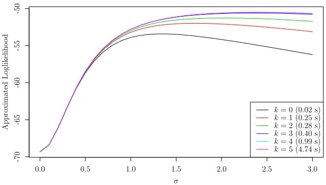
k= 0 (0.02 s) k= 1 (0.25 s) k= 2 (0.28 s) k= 3 (0.40 s) k= 4 (0.99 s) k= 5 (4.74 s)
Fig 3. Sequential reduction approximations to ℓ(β = 0, σ), for various values of k. The curve for k= 0(the Laplace approximation) is the lowest line, and the lines get higher ask increases. The curves fork= 4andk= 5are indistinguishable.
If we include all covariates suggested by Turner and Firth (2012) in the model, the maximum likelihood estimator is not finite. A penalized version of the likelihood could be used to obtain a finite estimate. In a generalized linear model, the bias-reduction penalty of Firth (1993) may be used for this purpose. Further work is required to obtain a good penalty for use with generalized linear mixed models.
4.3. A three-level model
Rabe-Hesketh, Skrondal and Pickles (2005) note that it is possible to simplify computation of the likelihood in models with nested random-effect structure. Using the sequential reduction method, there is no need to treat nested models as a special case. Their structure is automatically detected and exploited by the algorithm.
We demonstrate the method for a three-level model. Observations are made on items, where each item is contained within a level-1 group, and each level-1 group is itself is contained in a level-2 group. The linear predictor is modeled as ηi=α+βxi+σ1ug1(i)+σ2vg2(i),whereg1(i) andg2(i) denote the first and
second-level groups to whichibelongs. We consider the case in which there are 100 second-level groups, each containing two first-level groups, which themselves each contain two items. The posterior dependence graph of this model is shown in Figure 1c, and has treewidth 2. The treewidth of the posterior dependence graph for a similarly defined L-level model isL−1.
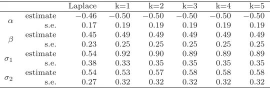
[image:16.612.114.444.111.299.2]Table 2
The parameter estimates and standard errors for the three-level model
Laplace k=1 k=2 k=3 k=4 k=5
α estimate −0.46 −0.50 −0.50 −0.50 −0.50 −0.50 s.e. 0.17 0.19 0.19 0.19 0.19 0.19
β estimate 0.45 0.49 0.49 0.49 0.49 0.49 s.e. 0.23 0.25 0.25 0.25 0.25 0.25
σ1 estimates.e. 0.540.38 0.920.33 0.900.35 0.890.35 0.890.35 0.890.35
σ2 estimates.e. 0.540.27 0.530.32 0.570.32 0.580.32 0.580.32 0.580.32
values found using the sequential reduction method with various different values of k are shown in Table 2. The parameter estimates found from the Laplace approximation to the likelihood are some distance from the maximum likelihood estimator, especially for the variance parameter of the level-1 group.
5. Conclusions
Many common approaches to inference in generalized linear mixed models rely on approximations to the likelihood which may be of poor quality if there is little information available on each random effect. There are many situations in which it is unclear how good an approximation to the likelihood will be, and how much impact the error in the approximation will have on the statistical properties of the resulting estimator. It is therefore very useful to be able to obtain an accurate approximation to the likelihood at reasonable cost.
The sequential reduction method outlined in this paper allows a good approx-imation to the likelihood to be found in many models with sparse structure — precisely the situation where currently-used approximation methods perform worst. By using sparse grid interpolation methods to store modifications to the normal approximation used to construct the Laplace approximation, it is pos-sible to get an accurate approximation to the likelihood for a wide range of models.
Acknowledgements
I am grateful to David Firth for useful discussions, and to a referee for helpful comments that improved the paper. This work was supported by the Engineer-ing and Physical Sciences Research Council [grant numbers EP/P50578X/1, EP/K014463/1].
Supplementary Material
R code for sequential reduction
References
Barthelmann, V., Novak, E. and Ritter, K. (2000). High Dimensional Polynomial Interpolation on Sparse Grids.Advances in Computational Math-ematics12 273–288. MR1768951
Besag, J. (1974). Spatial Interaction and the Statistical Analysis of Lat-tice Systems. Journal of the Royal Statistical Society: Series B 36192–236.
MR0373208
Bodlaender, H.and Koster, A.(2008). Treewidth Computations I. Upper Bounds Technical Report, Department of Information and Computing Sci-ences, Utrecht University.
Bodlaender, H.andKoster, A.(2010). Treewidth Computations II. Lower Bounds Technical Report, Department of Information and Computing Sci-ences, Utrecht University. MR2829452
Bradley, R. A. and Terry, M. E. (1952). Rank Analysis of Incomplete Block Designs: I. The Method of Paired Comparisons. Biometrika 39 324– 345. MR0070925
Breslow, N. E.andClayton, D. G.(1993). Approximate Inference in Gen-eralized Linear Mixed Models.Journal of the American Statistical Association 889–25.
Firth, D. (1993). Bias Reduction of Maximum Likelihood Estimates. Biometrika80 27–38. MR1225212
Fong, Y.,Rue, H.andWakefield, J.(2010). Bayesian Inference for Gener-alized Linear Mixed Models. Biostatistics11 397–412.
Jordan, M. I. (2004). Graphical Models. Statistical Science 19 140–155.
MR2082153
Mosteller, F. (1951). Remarks on the Method of Paired Comparisons: I. The Least Squares Solution Assuming Equal Standard Deviations and Equal Correlations.Psychometrika163–9.
Murarasu, A., Weidendorfer, J., Buse, G., Butnaru, D. and
Pfl¨uger, D. (2011). Compact Data Structure and Scalable Algorithms for the Sparse Grid Technique. SIGPLAN Notices4625–34.
Ogden, H. E. (2015). Supplement to “A sequential reduction method for in-ference in generalized linear mixed models”. DOI:10.1214/15-EJS991SUPP.
Pinheiro, J. C. and Bates, D. M. (1995). Approximations to the Log-Likelihood Function in the Nonlinear Mixed-Effects Model.Journal of Com-putational and Graphical Statistics 412–35.
Rabe-Hesketh, S.,Skrondal, A.andPickles, A.(2005). Maximum Like-lihood Estimation of Limited and Discrete Dependent Variable Models With Nested Random Effects.Journal of Econometrics128301–323. MR2189555
Rue, H., Martino, S.andChopin, N. (2009). Approximate Bayesian Infer-ence for Latent Gaussian Models by Using Integrated Nested Laplace Ap-proximations. Journal of the Royal Statistical Society: Series B71319–392.
MR2649602
Shun, Z.andMcCullagh, P.(1995). Laplace Approximation of High Dimen-sional Integrals.Journal of the Royal Statistical Society: Series B57749–760.
R Core Team (2014). R: A Language and Environment for Statistical Com-puting R Foundation for Statistical ComCom-puting, Vienna, Austria.
Thurstone, L. L. (1927). A Law of Comparative Judgment. Psychological Review34273–286.
Tierney, L. and Kadane, J. B. (1986). Accurate Approximations for Pos-terior Moments and Marginal Densities.Journal of the American Statistical Association8182–86. MR0830567
Turner, H. L. and Firth, D. (2012). Bradley-Terry Models in R: The BradleyTerry2 Package.Journal of Statistical Software48.