Possible strain scaling relation for YBCO superconductors?

Possible strain

scaling relation

for YBCO

superconductors?

Bachelor assignment report

Tim Mulder and Melanie Ihns

Guidance by Dr. M. Dhallé

Research Group EMS (Energy, Materials and

Systems)

Bachelor Applied Physics

[1]

Abstract

Superconductors have been investigated for a long time. But since the discovery of high temperature superconductors first in 1986, there has been done more research on low temperature superconductors than on HTS. So the behavior in the low temperature region of superconductors is already well known, but because industry aims to work with superconductors with increasing temperatures now high temperature superconductors have to be investigated.

For high temperature superconductors there is up to now no widely accepted theory how superconductivity occurs. There is no cooling of the atoms which reduces the lattice oscillations as in the case of low temperature superconductors and so it shouldn‟t be possible for electrons to follow all the same path and so having no resistance in the superconductor. Adding strain to a superconductor causes another change in the crystal lattice. The aim of this bachelor assignment is to explore whether it is possible to find a strain scaling relation for yttrium barium copper oxide (YBCO) superconductors.

When a material becomes mechanically strained, the crystal lattice becomes distorted. This influence is directly observable in the superconducting properties. These properties are best described with the so called critical surface of a superconductor. Not only the temperature is a critical parameter for superconductivity, but also the current and the applied magnetic field. This so-called critical surface will be constructed for the high temperature region of YBCO, which will be from 89K to 92K, for different magnetic fields (from 0T to 0.3T) and different values of strain.

The critical current and critical temperature found for different values of magnetic field in both the compressive and tensile strain region show non-linear behavior, peaking in both the compressive and tensile strain region. These finding match the finding of other groups researching the strain behavior of YBCO.

[2]

Acknowledgements

Hereby we would like to take the opportunity to thank the research chair Energy, Materials and Systems (EMS) for the support during this Bachelor assignment. In the first place we would like to thank Dr. Marc Dhallé who helped us to solve every problem and who worked several hours overtime to make everything working for our measurements. He helped us to find the right way through all the measurements and also during the phase of writing to select which datasets were more or less important and how to combine them. With his commitment he gave us a strong impetus when measurements were not working or long time had to be spent on preparation for the following experiment. In the surrounding of scientific research we could learn what working in the lab really implies. It‟s not just

[3]

Table of Contents

Abstract ... 1

Acknowledgements ... 2

1. Introduction ... 4

1.1 – Assignment ... 4

1.2 – Motivation ... 6

1.3 – State-of-the-art... 8

2. Experimental aspects ... 11

2.1 – Sample description ... 12

2.2 – Experimental strategies... 12

2.3 – Experimental Setup ... 13

2.4 – Data Processing ... 17

3. Results ... 18

3.1 – Critical temperature in dependence of applied magnetic field ... 18

3.2 – Critical current in dependence of applied magnetic field and temperature ... 21

3.3 – Construction of the critical surface ... 23

4. Discussion ... 25

4.1 – The scaling ... 25

4.2 – Data analysis for scaling relation ... 27

4.3 – Is it possible to scale? ... 30

5. Conclusion and recommendations ... 31

5.1 – Conclusion ... 31

5.2 – Recommendations ... 32

5.3 – Points of improvement ... 32

6. Nomenclature and Abbreviations ... 33

7. References ... 35

[4]

1. Introduction

1.1 – Assignment

The aim of this bachelor assignment is to explore whether it is possible to find a strain scaling relation for yttrium barium copper oxide (in the following referred to as YBCO) superconductors. The different aspects of this assignment will be now clarified one-by-one. Superconductivity can be described by the fact that below a critical temperature the magnetic field is repelled out the bulk material and only covers its surface. It means also, that there is instantly no electrical resistance in the material anymore when the temperature is beneath a critical value and so then there is no loss of energy. Here we distinguish between high- and low temperature superconductors (HTS and LTS), where the first already become superconducting at temperatures around 77K, the latter only in the neighborhood of 4.2K. The probably best known HTS is yttrium barium copper oxide which has a critical temperature of 93K. It is a copper-oxide

superconductor with a crystal structure as can be seen in figure 1. The whole structure represents one unit cell of YBCO where there is only one yttrium atom in the middle. Polycrystals of YBCO cannot sustain a high current density which is due to the grain boundaries in the material. If the angle between different crystals is larger than 5°, the supercurrent cannot cross the boundary and so superconductivity gets lost. In such a case only with single YBCO crystals superconductivity can be achieved for higher currents. This problem has been overcome essentially

by implementing epitaxial thin film technology on km-long substrates [1]. The resulting flat tapes are called “coated conductors” and are nowadays produced commercially. In this assignment such a commercial tape is studied, which is described in more detail in section 2.1 of this report.

How superconductivity occurs is for low temperature superconductors described by the BCS-theory, developed by John Bardeen, Leon N.

Cooper and John R. Schrieffer in the year 1957. However, for high temperature superconductors there is up to now no such widely accepted theory. The BCS-theory claims that the crystal lattice of the superconductor changes when the first conduction electron moves through it. With the change of the crystal lattice while electrons are moving along, there are phonons (oscillations) created, which produce a majority of positive charge in the distorted area. Due to electromechanical attraction

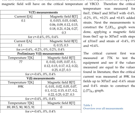
Figure 2 Cooper Pair [3]

Figure 1

[5]

the subsequent electrons are now more likely to follow the first one on the same path by which there are electron pairs formatted, so called cooper pairs (see figure 2). These cooper pairs are in the lowest possible energy state due to which they couldn‟t transfer energy to atoms they could impinge with. The atoms on the other hand also have to less energy to transfer it to the electron. The low energy of the atoms comes due to the low temperature at which the material becomes superconducting. Eventually electrons and atoms cannot exchange energy and so don‟t clash with each other, because then there would have to be energy exchange. We can imagine this low energy with a minimization of atom oscillations by cooling the superconductor down to almost absolute zero. Because the electrons all follow the same path, which is “prepared” for them by the first electron and because they do not scatter in the lattice, there is no resistance which else arises due to scattering of the electrons in the lattice [4]. But the low energy of the atoms gives exactly the critical point for high temperature superconductors, because here we have due to the higher temperature a higher energy and energy exchange to the electrons would be possible, so that there would have to be a resistance and the formation of cooper pairs shouldn‟t be possible; but still this is the case.

Although it is clear that this co called electron-phonon picture is not capable of explaining the occurrence of superconductivity in HTS materials [5], here it has been described mainly to show the basic origin of strain-dependence of the superconducting properties. When a material becomes mechanically strained, on a microscopic level the crystal lattice becomes distorted. This will have an influence on the behavior and energy of both phonons and electrons. As will be discussed in section 3.1 this influence is directly observable in the superconducting properties.

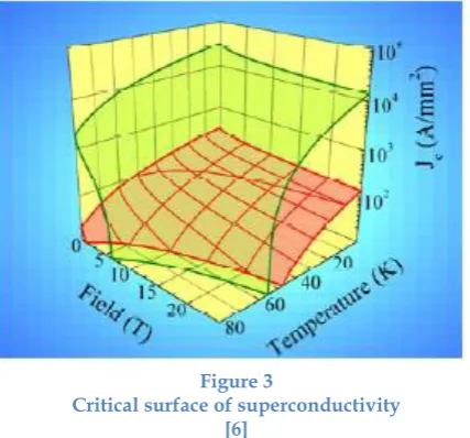
These properties are best described with the so called critical surface of a superconductor. Not only the temperature is a critical parameter for superconductivity, but also the current and the applied magnetic field. With this threefold dependence a critical surface can be drawn which shows the interface between superconductivity and non-superconductivity (see figure 3). Note that instead of current, one usually cites the so-called critical current density, where the cross sectional area over which the current is running is taken into account. Depending on the value of the applied magnetic field, the current density and the temperature we can say if the material will be superconducting or not. As long as the combination of B, J and T remains below the surface, the material is in the superconducting state. As soon as one of these three parameters becomes too large, we cross the surface and a transition to the normal state occurs. If there is strain applied on the material, the crystal lattice will change and so possibly also the superconducting properties. Whether the strain is stress, compression, torsion or bending is not important for the essence of the matter, only the critical values may change differently

Figure 3

[6]

depending on the kind of strain.1 _{Depending on the amount of strain the critical values of} temperature, magnetic field and current density also may change, so that under strain the needed temperature lowers even more or may be even higher than without strain. The critical surface and the reaction to applied strain of course depend on the crystal lattice of the material, so for all materials these values differ because of differences in the crystal lattice. There is also internal strain which occurs for example due to change in temperature that is thermal strain.2

It is important to know how materials react when applying strain. This can be done by measuring the critical values for different temperatures, magnetic fields and strain with a high data density, but that would represent a laborious and costly research effort. A better option is trying to “scale” all the data, so that the critical values are described by a single expression including the critical current, temperature, magnetic field and strain.

The term scaling refers to the shape of the critical surface under strain. If this shape remains essentially unchanged, i.e. if strain causes the surface to expand or to shrink in such a way that it retains its form, the superconducting properties are said to scale with strain and the description of strain effects becomes straightforward. This will be illustrated in a more quantitative fashion in section 1.3 below.

Strain scaling is known to hold in other superconductors, such as Nb3Sn and MgB2, which are BCS-like electron-phonon superconductors.

In HTS materials such as YBCO, however, the possible existence of scaling behavior has not yet been established. And this is precisely the starting point of this Bachelor assignment. The task was to make preliminary measurements to see if such a scaling relation can be constructed for YBCO.

In this Bachelor assignment the critical values of a thin piece of YBCO tape is measured. Critical surfaces will be constructed and if possible the results will be used to find a strain scaling relation as for other superconductors, in which a systematic and universal change in the critical current due to changes in external applied strain, temperature and magnetic field will be expressed.

1.2 – Motivation

Before getting into the details, however, let‟s consider why the presence or absence of scaling relations is important. In other words, what is the motivation behind this research assignment? Strain scaling is important both for fundamental scientists and for application-oriented engineers.

From a fundamental point of view, as mentioned before, for high temperature superconductors there is up to now no widely accepted theory how superconductivity

1 _{If the strain is too large, there is too much pressure on the crystal lattice, so crystal defects and}

eventually microscopic cracks will arise, which cannot be restored when returning the strain to zero. These are called irreversible strain effects. This assignment does not consider this “damage” regime, but limits itself to relatively low strain levels, where all effects are reversible.

2 _{But in this assignment it will be disregarded because it cannot be determined for our type of samples}

[7]

occurs. Here we don‟t have cooling of the atoms which reduces the lattice oscillations in the case of low temperature superconductors and so it shouldn‟t be possible for electrons to move in pairs and follow all the same path. Adding strain to a superconductor will also change its lattice constant, so then there are different formations in which the electrons can behave differently. Although a proper description of strain effects will not automatically lead to a better understanding of the interactions leading to superconductivity in HTS materials, it will provide a clear „test case‟ for the theoretical solid-state physicists. In order to be valid, any theory should be able to explain the observed experimental strain behavior satisfactorily. What‟s more, lattice deformation effects may even provide an intuitive guide to formulate theoretical explanations. Indeed, the discovery of superconductivity in YBCO itself is claimed to originate in considerations of lattice strain.

From a practical point of view, it hardly needs explaining why a concise description of strain-induced changes in the critical surface (i.e. a strain scaling relation) is important. HTS materials are being applied in an increasing number of devices, and all of them involve some level of mechanical loading (Lorentz forces) under widely varying operational conditions J, B and T.

Before getting into the details, however, let‟s consider why the presence of absence of scaling relations is important. In other words, what is the motivation behind this research assignment?

Strain scaling is important both for fundamental scientists and for application-oriented engineers. Superconductivity was discovered in 1911 by Heike Kamerlingh Onnes. In that time it could only be reached at temperatures under 4.2K. Around 1986 another type of superconductor was found, the ceramic high temperature superconductor (HTS) which already became superconductive at temperatures round the boiling point of nitrogen, 77K. These superconductors are better applicable for daily purpose because liquid nitrogen is a lot cheaper and easier to make than liquid helium, which was needed for low temperature superconductors. Superconducting materials with critical temperatures near room temperature are still a vision of the future and therefore the uses of superconducting materials are limited. The main use of superconductors today is its use in high field magnets, like the one in a MRI scanner, but also in bigger magnets like those in CERN and ITER.3 These electromagnets can produce strong magnetic field without any energy dissipation as heat, but need to be cooled to their critical temperatures with liquid nitrogen or liquid helium. As cooling systems are becoming much smaller and cheaper, superconductivity can be used easier for more applications. An important application for the future could be sustainable energy as for example in windmills. These are more and more set in the sea and therefore have to work reliably, because their maintenance is difficult. For this reason they have to be built with “direct drive” technology, what means, that the generator has to be connected directly to the blade axis. Right now this is realized with permanent magnets, but with superconductive magnets the same power could be reached within a much smaller volume [8].

3 _{Note, as an illustration of the importance of strain in applications, that the Lorentz force on the}

[8]

An important condition that has to be fulfilled is that a superconductor must not be brittle. Taking for example a superconducting generator for a wind converter, the superconducting wires have to be tightly wound into compact coils and are thus subjected to bending stress. Furthermore, in operation the coils in the generator windings are subjected to sizeable magnetic forces, which will again strain the material. If the superconducting attributes would disappear under strain the material would not be useful.

Fields produced by MRI scanners are relatively low and will not have much effect on the wire in the magnetic coil. But powerful particle accelerators, for example the Large Hadron Collider (LHC) at CERN, that is used to accelerate particles sufficient to cause a nuclear reaction, use high current magnets. The Lorentz forces created by the strong magnetic field from these electromagnets will exert radial force on each winding, pushing the wire outward adding strain on the wire. Also the cooling needed to reach the critical temperature of the wires in de magnetic coils adds thermal strain.

Another up and coming technology using superconductive wire is superconducting magnetic energy storage (SMES); this system can store energy in the magnetic field created by the flow of direct current in a superconducting coil. Storing energy in a SMES system has some advantages; it can output high power for short amounts of time and because of the zero resistance of the superconducting coil the SMES system is also highly efficient. These SMES system are currently used to maintain the stability of the power grid. By choosing HTS material for this device a few problems would appear. First of all the critical current and field of HTS are relatively low in the region of their critical temperature compared to those for LTS. So a HTS SMES system cooled with liquid nitrogen cannot store high currents, therefore sometimes it is chosen to cool the SMES system with liquid helium, making it far more expensive then a LTS SMES system. The second problem is that the strain tolerance of a HTS is less than that of a LTS; this is also restricting the use of a HTS. In the design of these devices using superconducting wires, mechanics should take into account that the critical surface of the superconductor will shift with added strain. Doing research on these critical surfaces is important for the optimal use of superconductors.

1.3 – State-of-the-art

Superconductors have been investigated for a long time. But since the discovery of high temperature superconductors first in 1986, there has been done more research on low temperature superconductors than on HTS. So the behavior in the low temperature region of superconductors is already well known, but because industry aims to work with superconductors with increasing temperatures now high temperature superconductors have to be investigated.

[9]

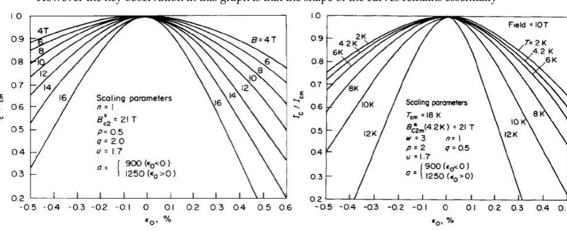
As the magnetic field B becomes higher, the curves become steeper and steeper.

However the key observation in this graph is that the shape of the curves remains essentially

unchanged. Mathematically this can be expressed by writing:

Where represents the shape of the master curve.

Figure 4b) reproduced also from [9], shows that a similar behavior was observed for the temperature dependence. Also here the curves become steeper and steeper as the temperature increases, but by normalizing T with a strain-dependent scaling temperature

, all curves can be made to collapse again.

Basically, this is the idea behind strain scaling of the whole critical surface: the surface may change more or less depending on temperature and magnetic field, but these variations are accounted for if we know how the 3 “corner points” of the surface with strain, i.e. if we know the scaling parameters , and . Details have been evolved since then, but the

essence of this description has been remained unchanged. The most recent published version of the strain scaling relations for Nb3Sn have been published by the ITER organization, who use the following relation for the design of their fusion magnets:

But this is only found valid for temperatures between 4.2K and the critical temperature, magnetic fields between 1 and 13T and strain values between -0.7 and 0.1% [10].

Using the same philosophy, the Low Temperature group in Twente where this assignment was carried out demonstrated scaling behavior in the most recently discovered technical

Figures 4 a) and b)

Relative critical current Ic/Icm of Nb3Sn as a function of intrinsic strain ε for different magnetic fields(left) and temperatures(right).

[10]

superconductor magnesium diboride MgB2 [11]. We will use the notation of this paper to extend the three-dimensional J-B-ε expression (1) to a more general four-dimensional J-B-T-ε formulation.

There is a general equation relating the change in critical current Jc to the change in applied

strain ε. This is a function of the current in dependence of the temperature T, magnetic field B

and strain, see equation (3).

The change in critical temperature and critical magnetic field due applied strain is simply the derivative of the dimensionless quantities and with respect to ε, see equations (4.a) and (4.b).

The change in critical current depends on the change of the critical temperature and critical magnetic field, see equation (5).

Filling equations (4.a) and (4.b) in into equation (5) gives the critical current dependence of the change in critical temperature and the change in critical magnetic field due strain, see equation (6).

For HTS, the available data are extensive but mostly do not focus on the strain-dependence of the critical current density at different

temperatures and different magnetic fields in both the tensile and compressive strain region.

Previously done measurements [12] have shown the behavior of YBCO for torsion and bending which yielded a symmetric relation of the irreversible current for positive and negative strain. Recently, Sugano [13], Cheggour [14] and Osamura [15] regarded the uniaxial strain effect and found for a

Figure 5

[11]

temperature of 77K a positive relation between low fields and the critical current in the positive strain region due to flux pinning. Flux pinning is “the phenomenon where a magnet‟s lines of force (called flux) become trapped or “pinned” inside a superconducting material” [16]. This is desired in high temperature superconductors because it prevents a pseudo-resistance to be created. But these experiments have mostly been done in the positive strain region, e.g. for stress on the YBCO tape. Sugano is the only one who also reported investigated effects for negative strain, i.e. compression and there he found in the high temperature region a second maximum of the critical current with respect to strain in the case of an applied magnetic field (see figure 4). The largest critical temperature up to now is found for mercury barium calcium copper oxide (HgBa2Ca2Cu3O9) at 138K and under pressure even at 160K [17].

For YBCO a scaling relation taking applied strain not into account is known from the master assignment of Frederik van Hövell [18] as:

[12]

2. Experimental aspects

2.1 – Sample description

The YBCO coated conductor used in this research is a commercial tape produced by SuperPower, that is 4mm wide, 35mm long and 0.095mm thick [7]. It is constructed in different layers including a copper stabilizer at the outside (see figure 6) in a continuous process using thin film

deposition techniques. The grain boundaries are aligned so that there are almost no obstructions for the current. The 50µm thick substrate is a high-strength Hastelloy substrate which makes the sample better appropriate for mechanical distortions. It also helps to prevent ferromagnetic current losses because the substrate is non-magnetic [7]. The actual YBCO layer is only 1µm thick, but the copper stabilization layers amount 40µm of the whole sample thickness. The YBCO tape is soldered on the u-shape sample holder described below, with also on the top a layer of SnPb solder to prevent oxidation. From the literature the largest possible strain that can be applied before crystal defects occur, is 0.52% tension and even -0.95% compression [20].

2.2 – Experimental strategies

To fully construct the critical surface two different measurement methods have to be used. The first method is to measure the

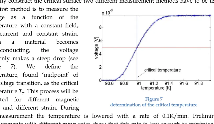
voltage as a function of the temperature with a constant field, low current and constant strain. When a material becomes superconducting, the voltage suddenly makes a steep drop (see figure 7). We define the temperature, found „midpoint‟ of the voltage transition, as the critical temperature . This process will be repeated for different magnetic fields and different strain. During

the measurement the temperature is lowered with a rate of 0.1K/min. Preliminary measurements with different ramp rates show that this rate is low enough to minimize the uncertainty in the temperature to ∆T ≈ 20mK.

Figure 6

YBCO coated conductor [19]

Figure 7

[13]

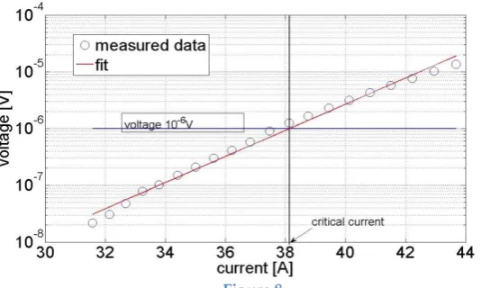
The second method is to measure the voltage as a function of the current through the sample, with constant magnetic field, temperature and strain. The current through the sample when the voltage over the sample reaches _{is defined as the}

critical current. This process will be repeated for different magnetic fields, different temperatures and different strain.

The data collected from these measurements will be enough to construct the critical surface for different values of strain. First the line will be constructed from the critical

temperature measurements. Next the line will be constructed and finally the line will be constructed from the critical current measurements. A few extra critical current measurements in the middle of the surface will be added to be able to fully construct the critical surface.

2.3 – Experimental Setup

The most important device for the measurements was the so called u-shaped sample holder (see figure 9), on which a piece of YBCO tape is soldered. Strain can be applied on the sample holder from outside the cryostat by a long rod which has to be turned to apply positive of negative stress on the legs of the sample holder (figure 10). This way the spring legs are either clenched, so that there is tension on the YBCO tape, or pushed apart, so that

Figure 9

Schematic drawing of the U-shaped sample holder [21] Figure 10

Photo of the U-shaped sample holder Figure 8

[14]

there is compression on the YBCO tape. On the sample holder there are strain gauges which measure the applied strain resistively. One is located on the outside of the u-shape and one on the inside of the u-shape, so that one of the two resistance values grows with increasing strain and the other will get lower (figure 9, bottom right).

The sample strain is described as a linear function of the measured strain values

.

The strain in both strain gauges is calculated with the following equation:

To determine the approximate gauge resistance needed to establish the desired strain in the sample the following equation is used:

The value of ε2, that is the value for zero strain at 92K, is equal to . The difference in resistance of strain gauge ε2 for a desired strain on the sample of -0.4%, -0.2%, +0.2% and +0.4% could be determined as , , and respectively.

The strain in the YBCO tape conductor was then later determined more precisely by filling the strain in both strain gauges in equation (8) after adding strain to the sample until the calculated resistance of strain gauge was reached.

Given the values for the two resistances,

and (the difference in

decimals is because of the use of two different

Figure 12 Cryostat that was used Figure 11

[15]

multimeters), the precise strain on the sample could be determined as , , and .

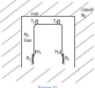
On top of the u-shaped sample holder two temperature sensors (T1&T2) are placed to measure the temperature of the sample. To raise the temperature of the material to its critical temperature the sample holder is partially insulated from the surrounding liquid nitrogen bath and two heaters (H1&H2) are placed on the sample holder, for each sensor one. The sample is insulated from the liquid nitrogen by shielding it with pieces of wool and a solid cup (figure 11). The cup is not only for heat shielding, but also so that a gas bubble can be created inside, allowing the temperature to go higher than 77K. The balance power between the heating power (PH) developed with the heaters and the cooling power

determines the sample temperature. The thermal resistances (R1&R2) are mainly determined by the current leads that feed the measuring current into the sample. Since these two leads are never perfectly balanced, an extra eternal variable resistor is placed in series with one of the heaters to lower its thermal output, so that the temperatures measured by the two temperature sensors on

both sides of the sample are equal (figure 13). For the first method of measuring (measuring the electrical resistance as a

function of the

temperature), low currents are used. Two small wires are soldered on the sample for applying current and two small wires for measuring the

voltage over the sample. With the second method high currents are applied on the sample, the two small wires are now replaced by placing two conducting “legs” on the sample holder, enabling higher currents to the sample. These two conducting legs are in direct contact to the liquid nitrogen, making them a larger thermal leak to the gas bubble inside the cup. This leads to a less stable temperature inside the cup.

The sample holder is placed inside a copper coil; this coil produces a magnetic field of 3.07mT per ampere, which is oriented perpendicular to the sample. In the experiment a maximum of 100A is used, producing a magnetic field of 307mT. The current through the coil is measured with a “zero-flux” device and is stable within 0.01 ampere. The coil is not made of superconducting material, so it produces a lot of heat when in use.

For the first method of measuring, the temperature is measured and controlled with a temperature controller, the voltage over the sample is measured with a nanovoltmeter, a small current is applied using a low-current source and both resistances from the strain gauges are measured with multimeters. The current for the magnet is provided with a high current source. To remove to offset from the nanovoltmeter, each measurement will be done

Figure 13

[16]

twice, once with a positive sample current and once with a negative sample current. Adding the resulting sample voltage values and then dividing them by two removes the offset from the measured voltage. The difference in between both measured temperatures (T1 and T2) is added as a measurement uncertainty in the temperature.

For the second method of measuring instead of a low current source, a high current source is used. The current is controlled by a computer program and measured with a second zero flux measuring system. Other measuring equipment is the same as in the first method. With this setup it is not possible to do the same trick used in the first method of measuring, sending positive and negative current through the sample. To remove to offset in this setup a few extra measurement without any current are needed. The mean offset measured is extracted from the values measured with current. There is still a small error in the temperature; it is not possible keep the temperature exactly stable at the temperature of choice, .

The critical temperature was measured for fields between 0mT and 307mT and strain from -0.4% to -0.4%. In this low field region the critical temperature will vary in the range of 89-92K. The first measurements were measurements to determine what impact strain and an applied magnetic field will have on the critical temperature of YBCO. Therefore the critical temperature was measured for 0mT, 154mT and 307mT with -0.4%, -0.2%, 0%, +0.2% and +0.4% added strain. Next the measurements to construct the graph were

done, applying a magnetic field from 0mT up to 307mT with steps of ±31mT and strain of -0.4%, 0% and +0.4%.

The critical current first was measured at 77K to test the equipment and see if the values measured are equal to the values found in literature, then the critical current was measured at 89K for fields up to 307mT and -0.4% strain and 0.4% strain to construct the

graph.

Table 1

Overview over all measurements

V(T) measurements

Current I[A] Magnetic field B[T] 0.1 0, 0.015, 0.03, 0.045, 0.06, 0.09, 0.12, 0.15, 0.18, 0.21, 0.24, 0.27,

0.3 for ε=-0.4%, 0%, 0.4%

Current I[A] Magnetic field B[T]

0.1 0, 0.15, 0.3

for ε=-0.4%, -0.2%, 0%, 0.2%, 0.4% Preliminary V(I) measurements

Temperature T[K] Magnetic field B[T] 77 0, 0.02, 0.05, 0.07, 0.1,

0.12, 0.15, 0.17, 0.2, 0.22, 0.25, 0.27, 0.3 for ε=-0.4%, 0%, 0.4%

V(I) measurements

Temperature T[K] Magnetic field B[T] 89K 0, 0.01, 0.02, 0.05, 0.07,

0.1, 0.12, 0.15, 0.17, 0.2, 0.22, 0.25, 0.27, 0.3 for ε=-0.4%, 0%, 0.4%

Temperature T[K] Magnetic field B[T] 89, 89.5, 90, 90.5, 91 0

[17]

After that the graph was constructed measuring the critical current for temperatures

between 89K and 92K at zero field. A few measurements between 89.5K and 90K and fields up to 200mT were done in all three strain states for the construction of the critical surfaces. Table 1 gives an overview of all measurements that were performed.

2.4 – Data Processing

The measurement data collection for the critical temperature was achieved with a LabView script that reads the temperature from the temperature controller and the voltage measured for each temperature value. For the critical current the data was measured with a Pascal based program “VI.exe”. With this application the data from all devices could be read and at the end of each separate measurement the data of mean temperature of both temperature-sensors, the magnetic field, the applied current, applied strain and the voltage over the sample were given.

As shown in figure 7, we define “the” critical temperature as the midpoint of the voltage transition. In order to determine this midpoint as accurately as possible, the curves for the voltage as function of the temperature were processed with Origin and fitted with the expression:

From this fit the critical temperature and the error in the critical temperature can be found. The curves for the current J versus the voltage V were processed with Matlab4 _{and linear} fitted with the expression:

From the fitted line through the measured data points the value for the critical current could be found as the point, where the curve crosses the voltage of _{. A Matlab script fits}

the data points and calculates the critical current automatically for all data in one datafile. With all data for the critical temperature, the critical current and the magnetic field the three critical surfaces for the different strain states could be found by generating x- and y-arrays for the plot of T and B, transforming the z-column (that is the critical current) into a matrix and plotting this against the values for critical temperature and magnetic field in Matlab.

[18]

3. Results

3.1 – Critical temperature in dependence of applied magnetic field

In first instance the critical temperature was determined in zero applied magnetic field from measurements of the voltage vs. temperature for different strain states from -0.4% to +0.4%. In a second step then these measurements were repeated at magnetic fields of 154 and 307mT. The resulting V(T) curves are shown in figure 14.

Figure 14

curves for critical temperature measurement

[19]

To compare these results in more detail, the critical temperature was extracted as the „midpoint‟ of the voltage transition, as described in paragraph 2.2. The resulting Tc(ε) values are plotted against strain for each of the three magnetic field values in figure 15. The error bars indicating the uncertainty of the Tc values are obtained from the fitting procedure

described in paragraph 2.4. All curves show a clear non-monotonic behavior. The „simplest‟ curve is measured at B=0 and shows one single maximum, the critical temperature with -0.2% strain applied is the highest in that curve. Further compression of the sample to -0.4% strain decreases the critical temperature again. Positive strain clearly has a negative effect on the critical temperature at zero magnetic field. In a magnetic field of 154mT the applied negative strain (-0.2% and -0.4%) clearly has a positive influence on the critical temperature, raising the critical temperature compared to that measured without any strain applied. In comparison to the values of the critical temperature without magnetic field, at 154mT the compressive -0.4% applied strain has a larger positive effect on the critical temperature than zero applied strain. The critical temperature measured with positive strain applied at 154mT still are lower than without any strain, but relatively got raised in comparison with the critical temperature measured at zero magnetic field. At 307mT however, these effects are significant and the Tc(ε) curve at this field shows the “richest” behavior with a local maximum at and a local minimum at . For negative strain, Tc increases monotonically.

Figure 15

[20]

Summarizing the Tc(ε) data at zero magnetic field the critical temperature has a peak around -0.2% strain. This peak shifts to the more negative strain region when applying magnetic fields of 154mT and 307mT. Also a second peak forms around the +0.2% applied strain. This peak is not as high as the peak in the negative strain region. In figure 16 in principle the same edge of the critical surface can be seen, the critical temperature is plotted against the

magnetic field with a high data density.

This relatively complex strain dependence contrasts with the situation in Nb3Sn (figure 4) and MgB2 (figure 17), where either a global

maximum or a monotonic dependence respectively is measured. To the best of our knowledge, there are no equivalent Tc(ε) data available in literature. However, there is one report about the in-field of strain dependence of Jc(ε) that shows similar features. Our results found with the critical temperature match the results found with the critical current by Michinaka Sugano [13]. Why the behavior of the critical temperature is like this couldn‟t be worked out in this bachelor assignment, because a lot more measurements at different strain states would have been necessary. Nevertheless Sugano suggests that the second

peak is caused by a flux pinning mechanism which only occurs at low magnetic fields,

Figure 16

critical temperature vs. magnetic field for three different strain states

Figure 17

[21]

because he measured also at higher magnetic field where the second peak diminishes more and more (see figure 5).

The insert of figure 16, 18, 19 and 20 schematically shows which part of the four-dimensional critical surface these experiments are probing, which will be further explored below in paragraph 3.3.

3.2 – Critical current in dependence of applied magnetic field and temperature

From the measurements with higher currents, two curves are constructed, one showing the dependence of the critical current on the applied magnetic field and one showing its dependence on the temperature.

Figure 18

[22]

Figure 18 shows the field-dependence of the critical current density at T=89K in

logarithmical scale, measured at three different strain levels. The Jc(B) values have been normalized with the value of Note that these curves show similar features as the Tc(ε) data reported in figure 15. Without any magnetic field the normalized critical current with applied strain starts around 0.60 with -0.4% and 0.36 with +0.4% strain (see figure 17). The critical current decreases logarithmical when applying a magnetic field. At a magnetic field of 154mT the critical current under applied strain of -0.4% is greater than the critical current without strain. For increasing magnetic field the critical current measured without any applied strain approaches the critical current measured for

0.4% applied strain. The critical current with zero strain does not get lower than the critical current measured with 0.4% strain for the different fields applied in this experiment, but we expect that by increasing the magnetic field further than 307mT there is a high probability that it will get lower.

Next we explore the behavior of the critical current with temperature, measured at zero magnetic field (figure 19). Once more, the data has been normalized with Je(B=0;ε=0;T=89K). It can be seen that the critical current decreases with negative as well as positive strain in all temperature regions. However, for zero applied strain the drop of critical current is much larger than that with applied strain. Compressive strain has a smaller negative influence on the critical current than tensile strain, so at 90.5K the sample has almost zero critical current at both states (0% and -0.4%), while under tensile strain this value is already reached at 90.0K.

Figure 19

[23]

3.3 – Construction of the critical surface

With the dependence of the critical temperature on the applied magnetic field (figure 16), the dependence of the critical current on the applied magnetic field (figure 18) and the dependence of the critical current on the temperature (figure 19) the edges of the critical surfaces of superconductivity for the three different strain values can be drawn. To determine the whole surface there were done some measurements of points within the three surrounding edges of the critical surface (see figures 20 and 21). With this data the entire critical surface can be constructed. Note that in the surface plot the critical current is not the normalized current anymore.

Figure 20

measurement of critical current at 89.5K

Figure 21

[24]

As can be seen in figure 22, at low magnetic fields and T=89K there is a relative big gab between the surface for 0% strain and the strained surfaces. When increasing the magnetic field, the surfaces approach eachother and the surface of -0.4% strain eventually even crosses the surface of 0% strain. The surface for 0.4% strain is the lowest surface in the measured region But by looking at the found data, decreasing the temperature further and raising the magnetic field it is probable the 0% strain surface also crosses the 0.4% surface and has the lowest critical current density in that region.

By looking at the the low magnetic field region between 89K and 91K, it looks like the surface of -0.4% strain crosses the surface of 0% two times. This is because of the surface fitting procedure, by looking at the raw data this overlap should only occur after 0.1T. Better surface fitting is possible with a higher data density, for this more measurements are needed.

Figure 22

[25]

4. Discussion

4.1 – The scaling

In the preceding chapter we have shown the results of the done measurements for the critical current and temperature for different strain states and the magnetic fields. All data has been combined to the surface plot for the three different strain states. The question of this bachelor assignment was whether this data could be translated into a mathematical strain scaling relation, i.e. whether the critical current can be determined as function of the three other parameters, the temperature, magnetic field and strain (equation 14).

If this can be expressed in the normalized relation (15), there can be spoken of scaling, because then the actual shape of the surface of the critical current in dependency on the temperature and the magnetic field remains the same for all strain states.

This hypothesis will be tested by looking on the behavior of the critical current for several values of the temperature and the magnetic field at different strain states.

As mentioned above the critical current is a function of all three parameters, with

The change in critical current in dependence on strain is directly related to the change in critical temperature, critical magnetic field and critical current, seen in (15). Mathematically this can be expressed in the partial derivative of JC (16) for strain with fixed values of

temperature and magnetic field. This results in the following equation:

The three derivatives to ε in (17) are the change in the critical parameters of the material and are key to the scaling process (figure 23). The solid black lines represent data of

measurements with MgB2 for zero applied strain. The arrows represent the change of the critical values due to strain.

[26]

Another important part of equation (17) is the shape of the critical surface j(b,t). The

normalized critical current j(b,t) for YBCO has been evaluated in the master thesis of Frederik van Hövell (see equation 7) [18] and serves as passable description of the dependency of the critical current on temperature and magnetic field without any strain applied.

with

and

with the fitting parameters:

[18]

The critical current is given here as a function of only temperature and magnetic field. The temperature is however also a variable for the pinning force and the irreversible magnetic field. The first brackets of equation (7) give again the normalized magnetic field above mentioned as b, but now not normalized with respect to zero strain, but with respect to temperature. It turns up again in the second brackets. In the first term of equation (7) there is the pinning force Fp0, which occurs due to crystal defects.

Note that the critical temperature used in these equations is 87.5K; this is even lower than then the used temperatures in our experiments. Trying to fit this function, of course with a higher value for the critical temperature parameter, did not give a good fit of the surface found in this experiment; possibly because this function was created from values found in

Figure 23

[27]

literature and a few extra measurements at low temperature. The high temperature region has not been accounted for when creating this function.

In paragraph 4.2 the measured data will be analyzed for a scaling relation and compared to the literature.

4.2 – Data analysis for scaling relation

To begin to find an answer to the question if there is a strain scaling relation there will be looked at equation (17) to find the dependence of the critical temperature and current on applied strain. The values of the critical magnetic field are not directly measured, but can be obtained by evaluating the Tc(B) and Ic(B) measurements.

Starting with the critical temperature, according to figure 24 where the dependence of the critical temperature on the applied strain can be seen it will be difficult to find a general relation because there is no linear behavior of the critical temperature.

Comparing the measured values for the critical temperatures with the data of Sugano for the critical current (figure 25) we will assume that the

Figure 25

Critical current dependency on strain [13] Figure 24

[28]

critical current and the critical temperature behave similar under strain. In both curves with applied magnetic field there appear two peaks at strain non-zero values and the value without strain tends to be a minimum even if this is quite close to the value for positive strain for a magnetic field of 0.15T in the measured data. The data without magnetic field applied shows a quadratic behavior, but even here the maximum isn‟t at zero applied strain but for the measured graph at -0.2% and in Sugano‟s data at about 0.1%. The difference of the absolute value could be because here there were only measured values for 0, ±0.2 and ±0.4% for applied strain and maybe with smaller steps the curve would have a different shape. Next in line is the critical currents, starting to look at the preliminary measurements for the critical current (figure 26) big differernces can be found when compating it with literature (figure 27).

In both the compressive strain and tensile strain region the values for the critical current are the highest with a magnetic field 0.05T giving at -0.4% strain and at 0.4% strain. When the measured graph is compared with the results found by Sugano, the first difference that is noticed the graph Sugano got is precisely mirror-inverted with respect to the y-axis. Sugano found higher values for in the tensile strain region, where in our result the highest result are in the compressed

Figure 26

Critical current dependency on strain at 77K [measured]

Figure 27

[29]

strain region. Sugano‟s finding with the same magnetic fields as in this experiment are in overall agreement with the values found with -0.4% strain, while with 0.4% strain they are totally off.

Now going on with critical current the measurements at 89K (figure 28). The same kind of shape can be seen as in figure 26.

Figure 28

Critical current dependency on strain at 89K [measured]

In both the compressive strain and tensile strain region the values for the critical current are the highest with magnetic fields between 0.2T and 0.3T (figure 28). The best value for was got with an applied magnetic field of 0.25T when applying -0.4% strain, giving . In the tensile strain region the best value for was got with an applied magnetic field of 0.3T when applying 0.4% strain,

giving . _{Figure 29}

[30]

Comparing the values from figure 28 with the results found in Sugano‟s measurements at 83K (figure 29) big differences can be seen, keeping in mind the measurements in this experiment were done at 89K. Where Sugano found peaks around in the compressive strain region and peaks around tensile strain region, in this experiment peaks of with compressive strain and with tensile strain were found. It was expected to find higher values for when raising the temperature, as has been done at -0.4%, but finding such low values with 0.4% was quite unexpected.

From the shape of our measured data for the critical current, no conclusions can be drawn. Comparing it with the data with the data found by Sugano, it is probable the shape will be the same as the shape of his Jc(ε) curves if more measurements at more different values of strain would have been done. Now looking at both figure 26 and figure 28 where the dependence of the critical current on the applied strain can be seen it will be difficult to find a general relation because there is no linear behavior of the critical current. The critical magnetic field is assumed also to be non-linear, because being dependant on the current and temperature.

4.3 – Is it possible to scale?

[31]

5. Conclusion and recommendations

5.1 – Conclusion

The change in critical current and critical temperature of a uniaxially strained Cu coated YBCO tape conductor was measured for low magnetic fields in its high temperature region. A few conclusions are drawn from the results:

1. The critical temperature as a function of compressive and tensile strain with a constant magnetic field shows non-linear behavior in its low strain region; giving a peak value in both the compressive and tensile strain region. Because of this non-linear behavior, it was not possible to fit the data with the non-linear equation generally used for fitting LTS. The non-linear behavior of the values for the critical temperature matches the behavior of the values for the critical current found by Sugano.

2. The critical current found for different values of magnetic field and strain at 77K also shows non-linear behavior. This was expected, because the same measurements were done by Sugano. But the values found in the present experiments differ from the values found by Sugano. It is possible that the difference in results is caused by a different kind of coating applied on the YBCO layer.

3. The critical current found for different values of magnetic field in the three different strain states, i.e. -0.4%, 0% and +0.4% at 89K also shows non-linear behavior.

[32]

5.2 – Recommendations

In this bachelor assignment it was chosen to only construct the critical surface for three different values of strain: -0.4%, 0% and 0.4%. This gave a basic, but not profound insight into the effect of strain on the superconductive properties of YBCO. For a more profound insight into the strain dependence of the superconducting properties of YBCO more measurements with additional values of strain are needed. This was not done in this bachelor assignment, simply because there was limited time for measuring. Also, for deriving a strain scaling relation more measurements are needed. Given only the data from the done measurements no accurate relation can be derived. For further research on the scaling relation of YBCO it is also important not only to measure in the high temperature region, but also in the low temperature region. This will not only require the use of liquid helium, if measuring below 77K, but also the use of a superconducting magnet.

5.3 – Points of improvement

The high current source used for the measurements of the critical current in the high temperature region was not able to provide small current changes when working with low currents. For measurements at 77K there were no problems controlling the current source, because of the high critical current. But around 90K the critical current was so small ( ), that the current source did not react to the small difference in input voltage provided by a voltage source which was controlled by the computer. This resulted in a lot of measurements measured at the same current, while trying to change the current.

[33]

6. Nomenclature and Abbreviations

b [] dimensionless quantity for the value of the magnetic field with respect to the critical value

B [T] magnetic field

, Birr [T] critical magnetic field

Birr,0 [T] critical magnetic field for zero strain

BCS-theory theory developed by Bardeen, Cooper and John about superconductivity at low temperatures

CERN European Organization for Nuclear Research

ε [%] applied strain with respect to the zero state

ε1 [%] measured strain at the side of the U-shape

ε2 [%] measured strain at the bottom of the U-shape

εsample [%] resulting strain on the sample

EMS Energy, Materials and Systems

f(x) master curve

F0 [A*T*m-2_{] pinning force for zero strain}

Fp0 [A*T*m-2_{] pinning force at zero magnetic field} HgBa2Ca2Cu3O9 mercury barium calcium copper oxide

HTS high-temperature superconductor

ITER International Thermonuclear Experimental Reactor

JCo [A] current for zero strain

JC[A] critical current

[] normalized critical current

LHC Large Hadron Collider

LTS low-temperature superconductor

MgB2 magnesium diboride

[34]

Nb3Sn niobium tin

offset [V] offset voltage without current

R0 [Ω] sample resistance without strain

∆R [Ω] change in resistance due to applied strain

SMES Superconducting Magnetic Energy Storage

t [] dimensionless quantity for the value of the temperature with respect to the critical value

T [K] temperature

Tc [K] critical temperature

Tc,0 [K] critical temperature with zero strain

V [V] measured voltage

Vc [V] critical voltage

Vcorr [V] corrected voltage without offset Voffset [V] offset voltage for zero current

w0 [K] length of curvature at low temperature w1 [K] length of curvature at high temperature xc0 [K] point of curvature at low temperature xc1 [K] point of curvature at high temperature

[35]

7. References

[1] D. Larbalestier et al., High-TC superconducting materials for electric power applications,

nature, 2001, Volume 414, 368-377

[2] http://de.wikipedia.org/wiki/Yttrium-Barium-Kupferoxid, consulted on 20-05-2011 [3] http://www.ornl.gov/info/reports/m/ornlm3063r1/fig5.gif, consulted on

25-05-2011

[4] V. L. Ginzburg, Superconductivity, 1st ed., World Scientific Publishing Co. Pte. Ltd., Singapore, 1994

[5] D. Zaanen, High-temperature superconductivity: The secret of the hourglass, nature, 2011, Volume 471, 314-316

[6] M. Dhallé, A strain scaling relation for YBCO superconductors, description of the bachelor assignment

[7] http://www.superpower-inc.com/content/2g-hts-wire, consulted on 09-06-2011 [8] P. de Kuyper, „Prijs van supergeleiding is de koeling‘, UTNieuws, 19-05-2011, number 15,

5

[9] J.W. Ekin, Strain scaling law for flux pinning in practical aupersonductors. Part 1: Basic relationships and application to Nb3Sn conductors, Cyrogenics, 1980, Volume 20, 611-624

[10] A. Godeke et al., Experimental Verification of the Temperature and Strain Dependence of

the Critical Properties in Nb3Sn Wires, IEEE Transactions on Applied

Superconductivity, 2001, Vol. 11, 1526-1529

[11] M. Dhallé et al., Scaling the reversible strain response of MgB2 conductors, Supercond. Sci.

Technol., 2005, 18, 253-260

[12] T. Takao, Influence of Bending and Torsion Strains on Critical Currents in YBCO Coated Conductors, IEEE Transactions on Applied Superconductivity, 2007, Vol. 17, 3513-3516 [13] M. Sugano et al., The reversible strain effect on critical current over a wide range of temperatures and magnetic fields for YBCO coated conductors, Supercond. Sci. Technol., 2010, 23, 085013(1-9)

[14] N. Cheggour et al., Reversible axial-strain effect in Y-Ba-Cu-O coated conductors, Supercond. Sci. Technol., 2005, 18, 319-324

[15] K. Osamura et al., Force free strain exerted on a YBCO layer at 77K in surround Cu stabilized YBCO coated conductors, Supercond. Sci. Technol., 2010, 23, 045020(1-7) [16] http://www.superconductors.org/terms.htm, consulted on 25-05-2011

[17] R. van der Heijden, ‘Ijskoud het beste, de fascinerende toepassingen van supergeleiding’, Kijk, 2010, 1, 34-39

[18] F. van Hövell, Design estimates for a medium-sized SMES system based on different superconducting materials, Master thesis, Enschede, The Netherlands (2008)

[19] D.C. van der Laan et al., Large intrinsic effect of axial strain on the critical current of high-temperature superconductors for electric power applications, Applied Physics Letters, 2007, 90, 052506(1-3)

[36]

Appendix A

Mfile for reading and plotting the labview data of critical temperature

measurements

%% zonder veld %% compressie

close all; clear all; clc;

%e=-0.4%

x43=importdata('meting43.csv'); waarden43=x43./10000000; amplitude43=waarden43(:,3); temperatuur43=waarden43(:,1); % T_c=90.91+-0.02K % figure; % plot(temperatuur43,amplitude43)

% title('0.4% compressie zonder B-veld')

%e=-0.2%

x44=importdata('meting44.csv'); waarden44=x44./10000000; amplitude44=waarden44(:,3); temperatuur44=waarden44(:,1); % T_c=91.02+-0.05K % figure; % plot(temperatuur44,amplitude44)

% title('0.2% compressie zonder B-veld')

%% zonder rek

close all; clc;

%e=0%

x45=importdata('meting45.csv'); waarden45=x45./10000000; amplitude45=waarden45(:,3); temperatuur45=waarden45(:,1); % T_c=90.97+-0.01K % figure; % plot(temperatuur45,amplitude45) % title('0% rek zonder B-veld')

%% trek

close all; clc;

%e=0.2%

[37]

%e=0.4%

x47=importdata('meting47.csv'); waarden47=x47./10000000; amplitude47=waarden47(:,3); temperatuur47=waarden47(:,1); % T_c=90.56+-0.02K % figure; % plot(temperatuur47,amplitude47) % title('0.4% trek zonder B-veld')

%% B=300mT %% trek

close all; clc;

%e=0.4%

x48=importdata('meting48.csv'); waarden48=x48./10000000; amplitude48=waarden48(:,3); temperatuur48=waarden48(:,1); % T_c=89.47+-0.04K % figure; % plot(temperatuur48,amplitude48) % title('0.4% trek bij 300mT')

%e=0.2%

x49=importdata('meting49.csv'); waarden49=x49./10000000; amplitude49=waarden49(:,3); temperatuur49=waarden49(:,1); % T_c=89.54+-0.02K % figure; % plot(temperatuur49,amplitude49) % title('0.2% trek bij 300mT')

%% zonder rek

close all; clc;

%e=0%

x50=importdata('meting50.csv'); waarden50=x50./10000000; amplitude50=waarden50(:,3); temperatuur50=waarden50(:,1); % T_c=89.46+-0.05K % figure; % plot(temperatuur50,amplitude50) % title('0% rek bij 300mT')

%% compressie

close all; clc;

%e=-0.2%

x51=importdata('meting51.csv'); waarden51=x51./10000000;

amplitude51=waarden51(:,3); temperatuur51=waarden51(:,1);

[38]

% figure;

% plot(temperatuur51,amplitude51) % title('0.2% compressie bij 300mT')

%e=-0.4%

x52=importdata('meting52.csv'); waarden52=x52./10000000; amplitude52=waarden52(:,3); temperatuur52=waarden52(:,1); % T_c=89.69+-0.06K % figure; % plot(temperatuur52,amplitude52) % title('0.4% compressie bij 300mT')

%e=-0.4%

x53=importdata('meting53.csv'); waarden53=x53./10000000; amplitude53=waarden53(:,3); temperatuur53=waarden53(:,1); % T_c=90.05+-0.04K % figure; % plot(temperatuur53,amplitude53) % title('0.4% compressie bij 150mT')

%e=-0.2%

x54=importdata('meting54.csv'); waarden54=x54./10000000; amplitude54=waarden54(:,3); temperatuur54=waarden54(:,1); % T_c=90.00+-0.04K % figure; % plot(temperatuur54,amplitude54) % title('0.2% compressie bij 150mT')

%% zonder rek

close all; clc;

%e=0%

x55=importdata('meting55.csv'); waarden55=x55./10000000; amplitude55=waarden55(:,3); temperatuur55=waarden55(:,1); % T_c=89.91+-0.04K % figure; % plot(temperatuur55,amplitude55) % title('0% rek bij 150mT')

%% trek

close all; clc;

%e=0.2%

x56=importdata('meting56.csv'); waarden56=x56./10000000;

amplitude56=waarden56(:,3); temperatuur56=waarden56(:,1);

[39]

% plot(temperatuur56,amplitude56) % title('0.2% trek bij 150mT')

%e=0.4%

x57=importdata('meting57.csv'); waarden57=x57./10000000; amplitude57=waarden57(:,3); temperatuur57=waarden57(:,1); % T_c=89.82+-0.03K % figure; % plot(temperatuur57,amplitude57) % title('0.4% trek bij 150mT')

%% vergelijk alle lijnen

close all; figure;

plot(temperatuur53,amplitude53,'black',temperatuur54,amplitude54,'blue',tem peratuur55,amplitude55,'green',temperatuur56,amplitude56,'red',temperatuur5 7,amplitude57,'yellow',temperatuur52,amplitude52,'black',temperatuur51,ampl itude51,'blue',temperatuur50,amplitude50,'green',temperatuur49,amplitude49,

'red',temperatuur48,amplitude48,'yellow',temperatuur43,amplitude43,'black', temperatuur44,amplitude44,'blue',temperatuur45,amplitude45,'green',temperat uur46,amplitude46,'red',temperatuur47,amplitude47,'yellow')

title('change in critical temperature for different strain values at different magnetic fields');

xlabel('temperature [K]'); ylabel('voltage [V]');

legend('strain=-0.4%',

'strain=-0.2%','strain=0%','strain=+0.2%','strain=+0.4%','Location','NorthWest');

Mfile for plotting the critical surface

% plot kolommen

[40] x_rand_zonder=[89:dx:ceil(max(xzonder))]; y_rand_zonder=[floor(min(yzonder)):dy:ceil(max(yzonder))]; [X_zonder,Y_zonder]=meshgrid(x_rand_zonder,y_rand_zonder); Fzonder=TriScatteredInterp(xzonder,yzonder,zzonder); Z_zonder=Fzonder(X_zonder,Y_zonder); figure;

hold on;

axis([89 91 0 0.3 0 4]);

surf(X_zonder,Y_zonder,Z_zonder,'FaceAlpha',0.6,'FaceColor','red'); surf(X_min,Y_min,Z_min,'FaceAlpha',0.6,'FaceColor','yellow');

surf(X_plus,Y_plus,Z_plus,'FaceAlpha',0.6,'FaceColor','green'); hold off;

grid on;

xlabel('temperature [K]'); ylabel('magnetic field [T]'); zlabel('critical current [A]'); title('Critical Surfaces');

legend('strain=0%','strain=-0.4%','strain=+0.4%');

Mfile for analyzing a critical current measurement:

function [Ic,T,dT]=analysedata2(data)

% This Mfile will analyze a single Ic measurement, and will output the % critical current, temperature and the uncertainty in the temperature.

close all

format long

T = mean([mean(data(:,3)) mean(data(:,4))]);

dT = (max(max(data(:,3:4)))-min(min(data(:,3:4)))); l=length(data(:,1));

i=1; done=0;

while done==0

if sum(data([i:i+1],1)<[0;0])==2

offset=[data(i,2) data(i+1,2) data(end-1,2) data(end,2)]; waardes = [data(i+2:end-2,:)];

waardes(:,2)=waardes(:,2)-mean(offset); plot((waardes(:,1)),log(waardes(:,2)),'o') lastfit2 = showfit('y(x)=a*x+b');

Ic=(log(1*10^-6)-lastfit2.m(2))./lastfit2.m(1); done=1;

elseif i<l i=i+1; else Ic=0; done=1; end end

Mfile for importing a .VIP data file to matlab:

function tabel=importVIP2(fileToRead1,regels)

% This Mfile wil open a .VIP datafile and will output all measured data and % a summary of the critical current found for each measurement.