The Detection of Infarcted Stroke Tissue via
Localised Sodium Concentration Measurements:
A Non-Invasive Approach
By
Friedrich Wetterling
(M.Sc., Technical University of Ilmenau, Germany, 2005)
SUBMITTED TO THE SCHOOL OF PHYSICS, TRINITY COLLEGE DUBLIN IN PARTIAL FULFILLMENT OF THE REQUIREMENTS FOR THE DEGREE OF
DOCTOR OF PHILOSOPHY
Presented at
The University of Dublin
Trinity College
Supervised by
Dr. Andrew J. Fagan,
And
Prof. James G. Lunney
Summary
Quantitative 23Na Magnetic Resonance Imaging (qNa-MRI) is a non-invasive technique which has considerable potential for measuring Tissue Sodium Concentration (TSC) changes in pathological brain tissue states such as stroke or tumour. However, the quantification of 23Na with MRI has been hindered by limitations in Signal-to-Noise Ratio (SNR) within the required spatial and temporal resolution constraints. The aim of the work presented here was to develop a 23Na MRI resonator system with an optimal compromise between SNR and B1-field homogeneity to allow for accurate qNa-MRI, to
adapt an MRI sequence for short Time to Echo (TE) imaging, to apply the technique to an existing in vivo model of stroke in the rat brain, and to process the data to gain novel insights into the spatio-temporal TSC evolution after ischaemic stroke.
The design, development, and characterisation of a transceiver (TXRX) and a transmit-only receive-only (TORO) coil system are described. The developed coils were compared to a commercial double-tuned 23Na/1H TXRX surface coil. As a result, the developed double-tuned TXRX surface coil achieved two-fold SNR improvement in the
23
Na channel, while maintaining the high sensitivity in the 1H channel. Furthermore, the developed double-tuned 1H/ 23Na volume resonator achieved a B1-homogeneity better than
5 % across the sample volume. In conjunction with the developed 23Na receive-only surface coil, up to three-fold better SNR was achieved in sample depths of 12 mm, the depth of interest for rat brain imaging. In a second development phase, a 2D-radial sequence was optimised to shorten the TE after the 23Na excitation pulse to below 1 ms. A TSC quantification method was developed for the dual resonator system and tested on phantoms containing known 23Na concentrations. This technique was then applied to the measurement of TSC maps in vivo in a rodent model of cerebral ischaemia with a spatial resolution of 1.2 µl and a 10 min image acquisition time. Such high spatio-temporal resolution allowed, for the first time, for the study of regionally dependent TSC change in vivo with a quantification accuracy of approximately ± 10 mM for up to eight hours after stroke induction. In contrast to previous studies in this area, it was found that TSC increased immediately in core tissue, but was delayed by up to 4 h in tissue considered to be still-viable but at risk of infarction.
Declaration
I declare that this thesis has not been submitted as an exercise for a degree in any other university.
This thesis is entirely my own work, except for the advice and assistance in the acknowledgements.
I agree to allow the library of TCD copy or lend a section or this entire thesis on request.
Acknowledgements
I would like to express my gratitude to those who contributed to the successful running of the 23Na MRI experiments; without them, I could not have written this thesis.
Special thanks go to…
… Dr. Andrew Fagan, for warmly welcoming me to Ireland, which became a new home to me over the past four years, for taking me on as his PhD student, for giving me all the scientific and personal support I needed during the course of my PhD, for facilitating my development as a young scientist in the field of MRI by giving me the opportunity to participate at national and international conferences, and furthermore for contributing to the success of this thesis through setting-up fruitful collaborations with leading MRI groups in Ireland, the UK, and Germany.
…Prof. Mhairi Macrae, and Lindsay Gallagher for supporting MRI scanning of their well-developed in vivo intraluminal thread model at Glasgow University/ Scotland, UK.
…Dr. Sven Junge, for supporting MRI scanning at Bruker BioSpin in Ettlingen/ Germany, and for guiding me in the field of RF coil development.
…Martin Tabbert, for supporting the development of the double-tuned volume resonator.
…Dr. Oliviero Gobbo, for supporting MRI scanning at TCIN, Dublin/ Ireland.
…Dr. Jacinta Browne, for an introduction in to the world of tissue-parameter replicating phantoms and their preparation.
… Margaret, my girlfriend who I am inexplicably blessed by, and with who I went through the ups and downs of writing this thesis.
…John, Gerard, Donald, and Paul, my friends who I have shared the same house with and who I enjoyed many good pints of Guinness with.
To my beloved grandmother:
Ruth Wetterling.
W ithout her encouragement this thesis
Index
1 INTRODUCTION ... 1
1.1 THE PRINCIPLES OF MAGNETIC RESONANCE IMAGING... 1
1.2 THE NMRPROPERTIES OF 23NA IN BRAIN TISSUE... 5
1.3 RESONATOR SYSTEMS FOR 23NA MAGNETIC RESONANCE IMAGING... 7
1.4 23NA MAGNETIC RESONANCE IMAGING AND STROKE... 9
1.5 HYPOTHESIS... 12
1.6 DOCUMENT STRUCTURE... 13
2 MRI RESONATOR THEORY AND CHARACTERISATION... 15
2.1 NMRSIGNAL THEORY... 15
2.2 ELECTRO-MAGNETIC RESONANCE THEORY... 17
2.3 LOSS MECHANISMS... 18
2.4 RESONATOR DEVELOPMENT TOOLS AND TEST METHODS... 21
2.5 RESONANCE CIRCUIT DESIGN... 27
2.6 MRIRESONATOR CHARACTERISATION... 36
3 EMPIRICAL EVALUATION OF SHAPED SURFACE COIL SENSITIVITIES AT 79.4 MHZ... 43
3.1 INTRODUCTION... 43
3.2 METHODS... 44
3.3 RESULTS... 53
3.4 DISCUSSION... 59
4 THE DEVELOPMENT OF A DOUBLE-TUNED 23NA/1H TRANSCEIVER SURFACE COIL... 65
4.1 INTRODUCTION... 65
4.2 RESONATOR DESIGN AND DEVELOPMENT... 67
4.3 COIL CHARACTERISATION RESULTS... 74
4.4 MRIMAGING EXPERIMENTS... 75
4.5 DISCUSSION... 79
5 THE DEVELOPMENT OF A DOUBLE-TUNED 23NA/1H BIRDCAGE RESONATOR ... 85
5.1 INTRODUCTION... 85
5.2 RESONATOR DESIGN AND DEVELOPMENT... 87
5.3 COIL CHARACTERISATION RESULTS... 98
5.4 MRIMAGING EXPERIMENTS... 99
5.5 DISCUSSION... 101
6 THE DEVELOPMENT OF A 23NA RECEIVE-ONLY SURFACE COIL ... 103
6.1 INTRODUCTION... 103
6.2 RESONATOR DESIGN AND DEVELOPMENT... 104
6.4 MRIMAGING EXPERIMENTS... 109
6.5 DISCUSSION... 112
7 THE MEASUREMENT OF TISSUE SODIUM CONCENTRATION (TSC) AFTER STROKE.... 117
7.1 INTRODUCTION... 117
7.2 SHORT ECHO TIME ACQUISITION AND DATA RECONSTRUCTION... 121
7.3 THE QUANTIFICATION OF TSC ... 131
7.4 THE MIDDLE CEREBRAL ARTERY OCCLUSION (MCAO)MODEL... 141
7.5 RESULTS... 147
7.6 DISCUSSION... 152
8 THE DEVELOPMENT OF A NON-LINEAR MODEL FOR TSC INCREASE AFTER MCAO ... 157
8.1 INTRODUCTION... 157
8.2 THE DELAYED-EXPONENTIAL TSCMODEL... 158
8.3 THE PHYSIOLOGICAL INTERPRETATION OF THE DELAYED-EXPONENTIAL MODEL... 161
8.4 THE DETECTION OF INFARCTED STROKE TISSUE DURING THE ACUTE PHASE... 162
8.5 RESULTS... 164
8.6 DISCUSSION... 167
9 CONCLUSIONS AND OUTLOOK... 173
REFERENCES ... 177
Abbreviations
DC …direct current
emf …electro motive force
FA …flip angle
FoV …field of view
FLASH …fast low angle shot
GRE …gradient echo
i.d. …inner diameter
MCAO …middle cerebral artery occlusion MRI …magnetic resonance imaging
MTX …matrix
NMR …nuclear magnetic resonance Q-factor …quality-factor
qNa-MRI …quantitative 23Na MRI
RARE …rapid acquisition with relaxation enhancement
RF …radio frequency
RoI …region of interest SNR …signal-to-noise-ratio
TA …acquisition time
TE …echo time
TORO …transmit-only receive-only
TR …repetition time
TXRX …transmit-receive VoI …volume of interest Voxel …volume element
23
1
Introduction
Stroke is the third most common cause of death and disability in Ireland [1]. Local 23Na concentration changes are known, from non-MRI examinations dating back several decades, to directly correlated with pathological changes in stroke tissue [2]. There is as a result a growing interest in investigating whether such pathological changes may be detected using 23Na Magnetic Resonance Imaging (23Na-MRI), for example by measuring regional changes in 23Na concentration in the acute phase following a stroke [3-11]. However, the exact measurement of Tissue Sodium Concentration (TSC) via quantitative
23
Na-MRI (qNa-MRI) in rat stroke models has been hindered by limitations in Signal-to-Noise Ratio (SNR) within the needed spatial (< 4 µl voxel size) and temporal (< 10 min acquisition time) resolution constraints [12, 13]. In this chapter, the general principles of MRI, possible qNa-MRI resonator systems, the physical properties of the
23
Na nucleus in brain tissue, and the applicability of qNa-MRI to investigate stroke tissue are explained.
1.1
The Principles of Magnetic Resonance Imaging
1.1.1 The Basic Free Induction Decay (FID) Experiment
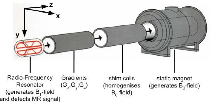
In Magnetic Resonance Imaging (MRI) the sample is exposed to a strong externally-applied magnetic field (B0), here 7.05 T. The basic components of the MRI
systems used for the work described in this thesis are presented in Figure 1.1. A superconducting electromagnet provides a static magnetic field, which points along the z-direction. A set of shim coils is then used to compensate for B0-field inhomogeneities
Figure 1.1: The basic components of an MRI system.
For the sake of simplicity, the principles of the MRI technique are explained based upon the properties of the 1H-nucleus, which is also used in common MRI techniques. The 1H spin (½) can occupy two energy levels due to the Zeeman interaction between the B0-field
and the proton’s magnetic moment (µ). The two energy levels can be interpreted as a parallel (↑↑) or antiparallel (↑↓) alignment of µ relative to B0. The occupation of these
states reaches a thermal equilibrium, which is described by the Boltzmann distribution:
=
↑↓ ↑↑ N N
kT E
e ∆
(Equation 1.1), where N↑↑/N↑↓ are the respective occupancy levels, ∆E is the Energy difference between the two states, k is the Boltzmann’s constant, and T is the temperature. The anti-parallel orientation is energetically less favourable leading to a slight excess of spins in the parallel alignment. The ensemble average of the magnetic moments of these excess spins results in a net magnetisation vector m0 with amplitude M0 aligned along the direction of B0, which
is usually defined to be the z-direction.
A second, time-varying magnetic field, the B1-field, is applied in the xy-plane
transverse to B0 in the form of a radio-frequency (RF) pulse generated by an RF coil. The
applied frequency of this RF-pulse is identical to the precessional frequency
ω
0 of thenuclear spins around B0, as described by the Larmor equation:
=
0
ω
γB0 (Equation 1.2),where γ is the gyromagnetic ratio. This RF pulse tips m0 away from the z-direction, while
orientation of M0 relative to B0. An RF pulse which tilts m0 from the z-axis into the
xy-plane is called a ”90˚
pulse”. After the transmission of a
90˚pulse, the nuclei precess in the xy-plane until the spin population relaxes to its equilibrium state, corresponding to a recovery of the net magnetisation along the z-axis. The MRI signal is measured as an induced voltage in a receiving RF coil – the MR signal - as long as there is a net magnetisation precessing in the xy-plane.1.1.1 Signal Properties
Two fundamental temporal parameters are used to describe the MR signal. The longitudinal relaxation time, T1, is the time constant describing the rate at which the
nuclear spins, once placed in a magnetic field, exponentially approach thermal equilibrium, so that the scalar component in the z-direction of the magnetisation vector is described by the formula:
( )
t =Mz
− −1
1
0
T t
e
M (Equation 1.3),
where M0 is the equilibrium magnetisation amplitude. In biological tissues, T1 for the
1
H-nucleus is long, ranging typically from hundreds of milliseconds to seconds. Differences in the T1 of tissues are one of the primary sources of image contrast in clinical
1
H-MRI.
A second time constant, T2, describes the transversal net magnetisation decay
following RF excitation. Small variations in the local magnetic field, for example those induced by the magnetic moments of neighbouring nuclei, cause the 1H spins to precess at slightly different frequencies and consequently to dephase relative to one another. Therefore, the T2-relaxation time relates to the spin-spin interaction. The observed signal
decay is described by the parameter T2*, which is the net transversal relaxation time which
is affected in turn by all the dephasing terms [14]:
=
* 2
1
T T2 T2inh T2suscept
1 1
1
+
+ (Equation 1.4),
where T2inhrepresents the dephasing due to magnetic field inhomogeneities and T2suscept is
the susceptibility-related signal loss depending on the sample’s magnetic susceptibility.
T2* generally ranges from a few milliseconds to tens of milliseconds.
Incorporating both T1- and T2-relaxation times, the MR signal, S(t), decays
( )
t =S 1 1 2*
0 T t T TR e e S − −
− (Equation 1.5),
where S0 is the signal strength immediately following the excitation pulse, and TR is the
repetition time between two consecutive RF-pulses. In imaging experiments, an additional parameter is used: the Echo Time (TE), which is defined as the time between the RF-pulse application (half pulse length) and the time point at which the maximum signal is acquired (typically of the order of milliseconds). TE has to be chosen appropriately long to let the differences in T2*or T1evolve before detecting the resulting signal. In the case of fast
decaying 23Na signals, TE must be chosen to be below 1 ms. By varying the TR and TE parameters, one can acquire images with contrast weighted by either the T1 or T2 relaxation
properties of the tissue under investigation.
1.1.1 Spatial Decoding
The MR signal detected originates from the ensemble net magnetisation of the entire sample volume. In order to form an image, the voxel-related net magnetisations must somehow be spatially resolved. This is usually a two-step process: (i) exciting the magnetisation in a single slice within the sample, and (ii) encoding the spatial location of the signal within this slice during data acquisition. This is done by using linearly varying magnetic fields in all three spatial directions to separate the signal from different locations according to a voxel-related frequency and phase difference. With a sample placed within a linear magnetic field gradient, for example, the Fourier Transform of the measured signal shows its strength at each frequency, and thus at each local position. Within the sample, MR imaging systems use three mutually orthogonal sets of gradient coils to generate these three gradient magnetic fields. The different gradients required are: slice selection Gz,
frequency encoding Gy, and phase encoding gradient Gx. Timing diagrams, for example
that illustrated in Figure 1.2, are used to describe the switching ON and OFF of the gradients, RF pulses and the timing of the data acquisition. These so-called “Pulse Sequences” have many variations leading to different image contrast (e.g. T1 or
T2) - Figure 1.2 illustrates a standard Gradient Echo (GRE) sequence as can be used for
23
Figure 1.2: The Gradient Echo pulse sequence (adapted from [15]).
1.1.2 Signal Variations and Noise
Noise is interpreted as increased variance with random amplitude in a measured image. There are two different types of noise in an MR image: low-frequency and wideband noise. The wideband noise is dominant for most MRI systems. It originates in the RF coil and is caused by thermal sources. Low-frequency noise typically exhibits a 1/f characteristic, and is composed of non-periodic, slow variations. In addition, periodic physiological noise can appear as peaks in the frequency spectrum. Any source of fluctuation such as body movements and spontaneous neural and vascular fluctuations contribute to the MRI noise and can decrease the SNR. The noise can effectively be reduced by reducing the coil dimensions, which is a standard design consideration when constructing RF coils, evident for example by choosing a dedicated coil for every part of the subject’s body (brain, knee, shoulder, etc.). Considering the sequence parameters, the sequence developer has to carefully choose the Acquisition Time (TA), as the SNR is proportional to the square root of TA and thus leads to the widespread use of signal averaging techniques in MRI.
1.2
The NMR Properties of
23Na in Brain Tissue
From a physics point of view, the sodium nucleus, 23Na, which has 100 % natural abundance, provides the strongest non-1H magnetic resonance signal that can be detected
invivo, and thus subtle changes in TSC can potentially be measured using qNa-MRI. The
23
levels when placed in a static magnetic field. In isotropic environments such as liquid solutions, the energy differences between all four energy levels are identical. The 3/2-spin number indicates that 23Na-nuclei possess an electric quadrupolar moment, which is due to the asymmetrical charges distribution in the nucleus. The energy differences between the outer Zeeman-energy levels change when sufficiently inhomogeneous electric fields, such as those produced by electron clouds and macro-molecules, exert detectable torques on those electric quadrupolar moments. Both the magnitude and the sign of the energy level shift of the external energy level transitions depend on the angle θ between the major axis of the quadrupolar tensor and the z-axis. If the local environment is isotropic, then averaging across all angles gives zero average energy displacement. In anisotropic environments such as in brain tissue or gels, quantum theory predicts that only 40 % of the total radiated energy contributes to the inner transition, decaying with a slow transversal relaxation time T2s, while the remaining 60 % corresponds to the two outer transitions,
decaying with a fast transversal relaxation time T2f [16]. This approximation also applies
for increasing 23Na concentrations, since the viscosity of NaCl solutions increases only slightly with increasing concentration; other NMR experiments have also shown that the contribution of electromagnetic field gradients from the 23Na and 35Cl ions to the relaxation are smaller compared to those from the electric dipole moments of the water molecules [16]. Thus, the environment in which 23Na nuclei are located influences the signal properties, with the 23Na signal detected from anisotropic brain tissue exhibiting bi-exponential decay due to the evolving electrical quadrupolar interaction. Shapiro et al. conducted measurements of such bi-exponential T2*-decay in agar gel phantoms, which
replicated thetissue environment of 23Na ions. As expected, the signal intensity decreased faster with increasing gel concentration in the 23Na environment [17].
Figure 1.3 shows the simulated transversal 23Na signal decay for tissue equivalent relaxation times, with T2s = 25 msand T2f = 5 ms. For standard TEs of 2 ms, the acquired
signal strength has already dropped by 25 %. Thus, identical 23Na concentrations contained in different tissue types may result in different measured MR signal intensity levels depending on the measurement time point after the RF excitation. Consequently, an exact knowledge of the tissue under investigation and its MR relaxation properties is essential for accurately quantifying the TSC. T2-weighting can then be minimised by
Figure 1.3: Simulation of the bi-exponential decay in tissue with total transversal relaxation time T2t, which is composed of the fast and slow exponential decays with fast T2f = 5 ms and slow T2s = 25 ms transversal relaxation times.
The NMR relaxation phenomena of spin 3/2-nuclei are complex for nuclei in aqueous heterogeneous system such as 23Na-nuclei in tissue. They are strongly affected by local binding and motions, and also by long-range ordering and the arrangements of the macromolecules [16]. Although quadrupolar interactions in biological tissue can be treated as a weak perturbation of the Zeeman interaction, the associated bi-exponential decay makes 23Na quantification difficult, when TEs longer than 1 ms are used.
1.3
Resonator Systems for
23Na Magnetic Resonance Imaging
single coil systems used as transmit-receive (transceiver) surface and volume resonators are discussed in the next paragraph.
The advantage of surface coils is that they can be placed very close to the signal origin on the sample’s surface and they thus detect the maximum possible signal strength. Surface coils were used by Thulborn et al. to investigate the rat brain [18], by Maril et al. to measure the TSC gradient across rat kidneys [19], and by Ouwerkerk et al. to image pathological brain and cardiac tissue in humans [20, 21]. Thulborn et al. had to compensate for B1-field inhomogeneities caused by the surface coil-dependent sensitivity
profile, whereby Ouwerkerk et al. and Maril et al. employed adiabatic pulses to gain more homogeneous B1-fields. However, the power deposition for such adiabatic RF pulses is
higher and the RF pulse lengths are longer compared to standard RF pulses, reducing the possibility of shortening the delay time between the RF-pulse and the data acquisition for qNa-MRI.
Volume resonators, on the other hand, generate a homogeneous B1-field, reducing
the need for B1-inhomogeneity compensation. Birdcage coils – a type of volume
resonators, have often been used for qNa-MRI, for instance by Constantinides et al. who used a single tuned birdcage coil for qNa-MRI on humans [22-24], Thulborn et al. who worked with a double tuned23Na/1H, dual quadrature birdcage coil for qNa-MRI on humans and non-human primates [8], Schepkin et al. who used a small birdcage coil (23 mm diameter and 45 mm length) to perform qNa-MRI on tumour in the rat brain [25], and Jones et al. who used a small dual quadrature, double tuned birdcage coil (5 cm diameter and 5 cm length) to determine the time of stroke onset in rats [5].
PAs compared to single receive-only surface coils remains to be verified for pre-clinical investigations on small bore MRI systems.
From reviewing the literature, a double-tuned 23Na/1H transceiver surface coil could provide maximised SNR for 23Na–MRI assuming one requires the capability to image 1H to allow for correlation of the 23Na images with high resolution 1H anatomical images. On the other hand, for qNa-MRI, a double-tuned 23Na/1H dual coil system composed of a 1H/23Na birdcage and a 23Na receiver-only surface could enable the TSC quantification in the rat brain, while maintaining a high SNR-efficiency in the 23Na channel and 1H imaging capability.
1.4
23Na Magnetic Resonance Imaging and Stroke
There are two broad categories of stroke, haemorrhage and ischaemia, which reflect diametrically opposite conditions: haemorrhage is characterised by too much blood within the skull, while ischaemia is characterised by a lack of blood and thus a lack of oxygen and nutrients supplied to a part of the brain [29]. The consequence of ischaemic stroke is slow necrosis, the death of tissue, which is also called infarction. The entire underperfused stroke lesion is generally subdivided into core (already infarcted) and penumbra tissue (still-viable and potentially salvageable). The immediate detection of infarcted stroke tissue after ischaemia via localised TSC measurements is the topic of the work presented here.
Brain tissue mainly consists of neurons, where each neuron encapsulates a small volume of intracellular (IC) space. The volume around neurons is referred to as the extracellular (EC) space, which in turn is composed of the EC compartment and the vascular compartment. Although the brain consists of more sophisticated anatomical structures, these are not considered in further explanations, because the physiological
23
Na concentration differs only between the IC and EC spaces (~ 10 mM and ~ 140 mM respectively [30]). The vascular compartment maintains the EC 23Na concentration at a constant level at all times even in diseased tissue. Thus, changes in cellular 23Na concentrations levels which for example occur following ischaemic stroke directly influence the overall Tissue Sodium Concentration (TSC).
excitation, when the membrane channels open to transmit the action potential along the axon. The Sodium-Potassium-Pump (Na+-K+-pump) re-establishes the concentration gradients afterwards. The energy for this is obtained from decomposing Adenin-Tri-Phosphate (ATP) into Adenine-Di-Phosphate (ADP). During cerebral ischaemia, the Na+-K+-pump function is disrupted leading to an increase of the IC 23Na concentration. Consequently, the TSC increases, while the EC 23Na concentration is maintained constant (~ 140 mM) through the vascular compartment and the kidneys.
It is clear from reviewing the literature that a variety of MRI techniques have been used to investigate ischaemic stroke. The vast majority of these are 1H-MRI-based, with diffusion MRI [10, 31, 32] predominantly used over perfusion MRI [18]. However, 23Na MRI approaches are beginning to be used, usually accomplished as T2*-weighted
23
Na-MRI [5, 18, 21, 25, 33, 34], while T1-weighted 23Na-MRI may also prove useful for
the detection of 23Na concentration changes [35].
A study comparing Diffusion-Weighted 1H-MRI (DWI), Perfusion-Weighted
1
H-MRI (PWI), and 23Na-MRI demonstrated that PWI is lacking in its ability to indicate disruptions in cell functionality [34]. The other two techniques demonstrated similar accuracies in localising areas of infarcted tissue. However, the temporal evolution of the abnormalities in ischaemic brain tissue detected by 23Na-MRI is different from that detected by T2*-weighted 1H-MRI and DWI related Apparent Diffusion Coefficient (ADC)
maps [11]. Jones et al. demonstrated that the increase of 23Na concentration which occurs during focal cerebral ischaemia can be measured with 23Na-MRI in the rat brain [5] and they went so far as to estimate an onset time of ischaemia, which has proved impossible to estimate using DWI. The aim of this project was to develop 23Na-MRI on a 7 T small bore MRI system in order to investigate the evolution of functional parameters during cerebral ischaemia in the rodent’s brain.
There are two different approaches using qNa-MRI to detect stroke in brain tissue: 1. Measuring the mean 23Na concentration, which is the Tissue Sodium Concentration
(TSC), and
2. Separately measuring the EC and IC 23Na concentration separately (using Chemical Shift Imaging or Multiple Quantum Coherences Weighting).
methods such as the Multiple Quantum Coherence (MQC) filters, allow for such splitting of the 23Na signals.
In CSI, the SR used is a paramagnetic anion, which cannot pass through the cell membrane, and hence does not enter the IC space. Once the SR reaches a certain compartment, it shifts the resonance frequency of only the 23Na ions contained in that compartment. It appears that the SR enters the EC-interstitial-space in every organ except the healthy brain, where it is constrained to the plasma space by the intact blood-brain-barrier [36]. CSI was used by Winter and Bansal, who used TmDOTP5- as the SR to mark the EC 23Na ions and to detect the IC 23Na signal in a brain tumour (9L gliasarcoma) [37]. The 23Na concentration was not quantified by MRI measurements, but rather transversal relaxation times of the EC 23Na ions were calculated by subtracting the measured IC 23Na signal in the presence of the SR from the measured total 23Na signal in the absence of the SR. They found that fast transversal relaxation with a time T2f occurs
extracellularly as well as intracellularly, with almost equally fast relaxation times at 9.4 T (IC: T2f = 2.0 ± 0.8 ms and EC: T2f = 3.4 ± 0.3 ms). Therefore, it cannot be assumed that
fast relaxation times of 23Na-nuclei occur only in the IC space, since they were also measured in the EC space, which exacerbates applying the MQC approach (see below). Neuberger et al. found the major disadvantage of CSI to be the inherently long data acquisition times required to acquire the 4-dimensional data sets that contain one spectral dimension and three spatial dimensions [38]. This meant that only a relatively sparse three-dimensional k-space matrix could be sampled. In conclusion, CSI can be used to shift the EC 23Na signal and thus can be used to measure the IC 23Na signal directly. In addition to the toxicity of all SRs used to date, applying CSI for brain in vivo
investigations is practically difficult, because they do not pass the blood brain barrier and would only reach their target if directly injected into the brain tissue.
The other method of splitting 23Na signals from the EC space and the IC space is to use MQC filters, which exploit the quadrupolar moment of 23Na to distinguish between
23
Pekar et al. suggested that multiple quantum filtration could be used to selectively observe the resonance from intracellular 3/2-spin metal ions [39]. Later, Kline et al. formulated that the presence of an MQC-signal could be used to identify populations of
23
Na nuclei by their molecular environment and could be used to detect changes in the IC space as they occur during cerebral ischaemia [40]. However, the signal intensity following a multiple-quantum spin sequence is only a small fraction of the signal intensity following a single, ideal, 90˚ excitation pulse (in vivo values of 10 % to 15 % have been reported [41]). This technique has also proven to be only partially successful, since it was found that EC ions also exhibit bi-exponential relaxation [42]. Nevertheless, MQC filters were successfully applied in imaging cartilage. Cartilage is strongly anisotropic compared to brain tissue and therefore possesses very short transversal relaxation time, which in turn result in strong MQC effects [43, 44]. Hancu et al. demonstrated the diagnostic applicability to image the normal human brain in vivo within 20 min using a three dimensional triple quantum filtered 23Na imaging sequence [45]. However,
B1-inhomogeneities [46], and B0-inhomogeneities [47] cause problems in MQC-MRI, and
the fast transverse relaxation times could not sufficiently be studied with currently available methods [16]. Practical complications were also mentioned by Goodman et al., who were unable to observe even-ordered 23Na coherences in rat brain tissue under optimised experimental conditions [48].
The measurement of MQC is still difficult due to a lack of conclusive results and a ten-fold lower SNR compared to TSC measurements. Thus, an SNR-optimised 23Na-MRI coil system may also contribute to novel insights in future MQC filtering experiments.
1.5
Hypothesis
1. The geometry and dimensions of a double-tuned transceiver surface coil can be optimised in a way that the detected SNR increases by more than 50 %, when compared to a commercially available planar surface coil (optimised for the
23
Na/1H-MRI rat brain application).
2. A dual coil system can be built, which generates a homogeneous B1-field at the
23
3. The TSC can be measured in a permanent in vivo rodent stroke model with a quantification accuracy and spatio-temporal resolution sufficient to detect subtle regional variations in TSC during the acute phase of cerebral stroke, using an optimised resonator system, sequence, and high static magnetic field strength (7 T).
1.6
Document Structure
2
MRI Resonator Theory and
Characterisation
23
Na Magnetic Resonance Imaging (23Na-MRI) suffers from low SNR caused by the
23
Na-nuclei’s low gyromagnetic ratio, low concentration in tissue and fast MR signal decay. The detectable 23Na SNR in the rat brain is furthermore restricted by the small voxel size (< 4 µl) which is required to spatially resolve structures such as the caudate-putamen and the cortex in the rat brain. Careful design of the detector systems with the specific sample dimensions and transmit pulse requirements in mind can therefore maximise the available SNR. The origins of the measured RF signal in the Nuclear Magnetic Resonance (NMR) experiment, the theory of RF circuit and resonator element design, and common characterisation techniques for room temperature MRI resonators are described in this chapter.
2.1
NMR Signal Theory
As described in Section 1.1, the RF resonance coil is used to apply a 90˚-pulse in order to tip the z-directed net magnetisation vector m0 into the orthogonal xy-plane, where it precesses while returning to its equilibrium orientation (along the z-direction). The induced electro motive force (emf) for a given geometric relationship between the detector coil and the sample location (see Figure 2.1) may be described as follows:
To enable the computation of the magnetic field strength originating from a sample location r0, the magnetic dipole moment must be converted to the equivalent magnetic
dipole moment, which is defined by a current flowing in a closed loop with surface area A:
=
0
Figure 2.1: The geometric relationship between the detector coil and the sample, where the sample is placed underneath the coil. The precessing net magnetisation vector in a particular sample voxel (illustrated at the right side of the image) induces an emf in the detector coil, which can be measured as a voltage drop-off across the coil terminals.
From this definition, the magnetic field strength at an arbitrary location on the coil’s detector surface having a distance r to the voxel position r0 can be determined via the Bio-Savart Law:
=
B
d 0 3 0
4 r r L Id
π
µ ×
(Equation 2.2), where µ0 is the permeability of free space, and I is the current in dL - the current flowing in
the loop formed by the equivalent magnetic dipole moment. The solution to this equation can be found elsewhere [49].
The final computation of the induced emf is based upon Faraday’s Law of electromagnetic induction. It states that the induced emf in a conductive loop equals the rate of change of magnetic flux through the loop [50], revealing that a time varying magnetic field strength threading through the conductive loop acts as a source of electric field and vice versa:
=
E
dt dΦB
− (Equation 2.3),
where E is the induced emf and ΦB is the magnetic flux threading through the conductive
loop at various time points t.
To compute the magnetic flux ΦB for the net magnetisation vector at one time
point, it is necessary to integrate over the magnetic field strength components (By), which
Thus, when the magnetic flux threading through the detector coil varies over time, as it does in MRI, a measurable emf is induced in the detector loop (Figure 2.2).
2.2
Electro-Magnetic Resonance Theory
The task of the MRI detector is to pick-up the induced emf during the MRI experiment and to transmit it as a voltage to the system preamplifier before further analogue-to-digital conversion and data acquisition. Careful design of this first element in the receiver chain is important to reduce signal losses during the measurements. Signal reflection for example can occur for cable lengths > λ/10 (where λ is the wavelength of the RF signal, which is related to the Larmor frequency and the velocity factor in the coaxial cable), when the cable and preamplifier impedances are mismatched. The detector impedance possesses complex impedance, which varies according to the coil environment, especially when placed inside the magnet on a variable load such as a rat’s head. Two main strategies exist to match the detector coil to the expected input impedance at the preamplifier (typically 50 Ω). The first option is to use another preamplifier directly at the coil terminals. The second and more commonly used approach is to exploit the electro-magnetic resonance effect at the desired Larmor frequency. The latter approach served for the development of various coil systems for 23Na- and qNa-MRI in this work and is described in the next paragraph.
The basic idea behind the electro-magnetic resonance circuit is to simplify the complex impedance by cancelling out the imaginary parts of the impedance of the resonance circuit, namely the inductance and capacitance. The real impedance can then be easily transformed to the cable and preamplifier input impedance, as described in Section 2.5.2 (‘Matching’) below. The impedance of a parallel LC resonator is composed of the complex capacitive and inductive impedances. The inductive impedance of the coil wire is
=
L
Z jωL (Equation 2.4),
with the angular frequency ω, and the conductor inductance L. The capacitive impedance with parallel capacitance C is defined as:
= C
Z
C jω
1
(Equation 2.5), Neglecting loss mechanisms, the frequency of such a resonance circuit is given by:
=
0 ω
LC
1
(Equation 2.6). This resonance equation demonstrates that the commonly employed parallel LC resonance circuit oscillates at one single frequency for which the magnetic energy stored in the inductor is exchanged for electric energy to be stored in the capacitor and vice versa. The resonance frequency is hence solely determined by the values of L and C, which can in practice be composed of several capacitive and inductive components, including parasitic capacitance between the coil and the sample.
The loss mechanisms, neglected above, are the reason why the resonance circuit inductance and capacitance for a desired Larmor frequency is difficult to be theoretically determined. Especially at high frequencies (> 1 MHz), the various loss mechanisms and interactions of the resonator with its conductive environment make it difficult to apply the loss-free resonance circuit approach. Therefore, the resonance frequency for the chosen element parameters must, in practice, be tuned through an iterative optimisation process, with the result monitored using a network analyser, which is explained in Section 2.4.2. Nevertheless, the knowledge of the loss mechanisms and their origin is of importance for the design of a well performing resonator. The loss mechanisms are explained in more theoretical detail in the next section.
2.3
Loss Mechanisms
which adds to the NMR signal-related emf. The effective noise signal magnitude σn in the
NMR experiment is mathematically expressed as:
=
n
σ 4⋅Reff ⋅kB ⋅T⋅∆f (Equation 2.7), where kB is the Boltzmann constant, T is temperature of the probe and ∆f the bandwidth of the detected NMR signal. The equivalent circuit diagram of the MRI resonance coil includes the losses as one effective loss resistance Reff in series with the coil inductance Lcoil. An optimum room-temperature resonator is thus characterised by its very low effective noise resistance and its ability to pick-up the highest possible emf.
Four different loss mechanisms contribute to the effective loss resistance, which are due to the antenna effect (radiation losses), the wire length (resistive losses), magnetic field carrying currents in the sample (magnetic losses), and parasitic capacitors arising between sample and coil (electric losses) [49]. The effective resistance representing the four loss mechanisms is computed additively:
=
eff
R RR+RΩ+RM +RE (Equation 2.8). The theoretical equations for the computation of the effective loss resistance are given in the next paragraphs.
The resistive resistance for a resonator made of conductive wire of length lwire, circumference cwire, conductivity κcoil, and skin depth δcoil is calculated via:
= Ω R wire coil coil wire c l ⋅ ⋅δ
κ (Equation 2.9),
The skin depth δcoil describes the frequency dependent penetration property of the electric current in metallic conductors and is computed as:
=
coil
δ
coil R ω κ
µ
µ0⋅ ⋅ ⋅
2
(Equation 2.10). where µ0 is the permeability constant in vacuum, µR is the permeability constant of the
material, and ω corresponds to the angular frequency.
Magnetic losses occur during the transmit phase and the application of a high current (typically in the range of 1 A) to the coil, which is driven by the high power amplifier. The transmitted B1-field generated by the resonance coil induces eddy currents
in the conductive sample. These eddy currents contribute to additive local magnetic fields within the sample with considerable influences on the total local magnetic field and thus the local flip angle. For a spherical sample of radius b, the calculation leads to
=
M
R M N2 2 b5
where MG is a coil geometry-related factor, N is the number of turns, and σ is the electric conductivity of the media used in the sphere.
An unbalanced coil starts to radiate some of the electromagnetic energy stored in the resonator to its environment. Such radiation losses occur due to the development of two resonance modes, one corresponding to the loop resonance and the other corresponding to an antenna of small dimensions. This effect is also known as the antenna effect. It becomes more evident for resonators with conductor lengths > λ/10, where λ is the RF wavelength in the conductor material. Thus splitting the conductor into multiple segments, as well as symmetrically arranging the circuit capacitors, can suppress the radiation losses [49].
Electric losses occur due to the close proximity of the resonance structure to the conductive sample environment. The electric field build up in capacitors penetrates in to the surrounding space and the conductive sample. Those electric fields drive currents through the sample and thus contribute to the electric loss mechanisms with:
=
E
R EG⋅ω3⋅L2 ⋅Cd (Equation 2.12), where EG is the geometry factor of the coil, and the coil is characterised by an inductive value L and a capacitive value Cd. Considering that the radiation and magnetic losses are very small during the receive period, the optimisation of receiver surface coils must focus on the minimisation of the resistive and electric losses, which is discussed in more detail below.
The resistive losses could potentially be reduced by the use of highly conducting materials such as silver or carbon nanowires [51]. However, the magnetic susceptibility of silver is very different from tissue and can cause MR signal distortions when brought near the sample. On the other hand, the highly conducting carbon nanowires could provide the ideal resonator material. Admittedly, the properties and macroscopic access to this novel material are still restricted. For this reason copper was preferred over silver or nanowires to develop MRI resonators for this project.
Varying the coil geometry and number of windings also has some potential with regards to increasing the detectable SNR. The measurable SNR benefit from the use of multiple inductor windings highly depends on the frequency and the dimensions-related loss mechanisms. As an example, one may express the increase in SNR obtained by doubling the number of windings as:
( )
( )
N =N emf
2 2
σ
( )
( )
( )
NN emf N c
σ
where N is the original number of windings, and c is the factor by which the SNR is increased. The induced emf doubles according to Faraday’s Law:
( )
N =emf 2 2⋅emf
( )
N (Equation 2.14). The measured noise voltage level at the coil terminals is related to the effective resistance (Equation 2.8) as follows:∝
n
σ Reff (Equation 2.15).
Since, the electric losses are proportionally to L2 (Equation 2.12), they increase by a factor of four, because L was doubled by the doubled number of windings N. However, the resistive losses are only directly proportional to N, resulting in an effective noise signal increase of:
( )
N =Reff 2
Ω ⋅ + ⋅RE 2 R
22 (Equation 2.16).
Considering that the electric losses are negligible for small detector dimensions and low resonance frequencies, it becomes evident that the effective noise levels for a doubled number of windings increases by approximately 40 %:
( )
2N =σ 2⋅σ
( )
N (Equation 2.17). Thus as long as the resistive losses dominate the electric losses and the conductor length is smaller than λ/10, doubling the number of windings can result in a SNR increasing factor:( )
N =c 2
( )
( )
( )
( )
22 2 = ⋅ ⋅ ⋅ N N N emf N emf σ σ (Equation 2.18). In the case of larger coil geometries (e.g. for human MRI), dielectric losses dominate the effective resistance and therefore multi-winding results in no effective SNR gain.
However, for small surface coils and low resonance frequencies, multi-winding must be considered to achieve the highest possible SNR. The fact of dominating resistive losses could furthermore be exploited through cooling the resonator coil and by these means limiting the temperature-dependent losses [52]. The fact that multiple winding coils for rat brain MRI at 79 MHz results in higher SNR was practically tested in this work (Chapter 3), exploited for the development of a transceiver surface coil (Chapter 4) and also used to develop a receive-only surface coil (Chapter 6).
2.4
Resonator Development Tools and Test Methods
network theory, where the developed LC resonator is treated as a black box with four connectors, which then is assessed by its ability to reflect and absorb electro-magnetic waves. The actual resonance frequency, the resonator’s quality-factor, and resonator coupling effects can thus be accurately characterised. The scattering parameter theory, the laboratory equipment used to characterise resonators, and the essential measurement methods for designing MRI resonators are described in this section.
2.4.1 The Scattering Parameters (s-Parameters)
Any electronic unit can be described by its frequency-dependent complex s-parameter set
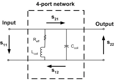
sab, when contemplating that the electronic unit is a black box with four connectors - an electric 4-port network (see Table 2.1). The s-parameter matrix is designed in a way that it relates the incident (-) and reflected (+) wave amplitudes at each port of the network. For the 4-port network shown in Figure 2.3, the s-parameters are defined as follows:
= − − 2 1 V V ⋅ + + 2 1 22 21 12 11 V V s s s s (Equation 2.19), where V1 and V2 are the voltage amplitudes measured in port 1 and 2, respectively. The reflected or output wave at each port is a function of the input waves at all ports:
= ab s 0 = + − + a V b a V V (Equation 2.20).
Out of the four s-parameters, the input reflection coefficient s11 and the transmission coefficient s21 are the most useful s-parameters for determining the resonance frequency and the matching properties of the LC resonator.
2.4.2 The Network Analyser
A network analyser is composed of a multi-frequency power signal generator, generating sinusoidal signals with temporally increasing frequency, an oscilloscope for measuring the reflected and transmitted voltage levels of an investigated circuit, and a processor for coordinating the interaction of both the generator and the oscilloscope.
Table 2.1: The terminology used to characterise 4-port networks by four s-parameters.
scattering parameter Notation
s11 input reflection s12 reverse transmission
s21 Transmission
Figure 2.3: The graphical interpretation of the scattering parameters in a 4-port network. The 4-port network circuit represents the equivalent parallel LC resonance circuit, which was used for this work.
Test objects with one or two ports can be connected to the network analyser. The scattering parameters can then be measured based upon the electric 4-port network theory. To measure the reflection and transmission, hybrids or diplexers are integrated into the test ports of the network analyser to separately detect the emitted and reflected waves. The attenuation between voltages is calculated using the formula derived from the decibel scale of power attenuation [50]:
=
) (sab
A
[ ]
dbV V b a ⋅ − + − 10 log
20 (Equation 2.21).
A network analyser can be used to measure the resonance frequency of an MR detector coil. Other coil characterising parameters, among them the Quality-factor (Q-factor), coil impedance, and transmission attenuation can also be measured. The network analyser used for this study was model E5061A (Agilent Technologies, USA). The following subsections describe how to measure the s11-reflection curve and Q-factor, and the s21-transmission curve of a resonance coil.
2.4.3 Pick-up Loops
(Figure 2.4). Pick-up coils were soldered to a corresponding SMB jack. The connections were insulated using heat shrink. Such an arrangement allows the coil designer to change pick-up coils easily without having too many wires on the work bench.
2.4.4 The Reflection Measurement
The reflection measurement is one of the most basic network analyser measurements, which allows for the determination of the resonance frequency and matching properties among other parameters of a LC resonator. In order to measure the s11-reflection attenuation, the LC resonator is connected to port 1 of the network analyser. By defining the centre frequency and the frequency span, the attenuation curve can be recorded as shown in Figure 2.5 for a 79.4 MHz surface coil; the centre frequency and span were chosen 79.4 MHz and 20 MHz, respectively. At the resonance frequency nearly all of the electromagnetic wave was absorbed by the resonator, which resulted in less than -30 dB
s11-reflection attenuation at 79.4 MHz, representing very good signal absorption. Almost no signal was absorbed at other frequencies, as indicated by the complete reflection of the incident wave at these frequencies (> -1.5 dB). This measurement allowed for the accurate determination of the resonance frequency of any LC resonator under real world influences such as resistive losses and loading effects (electric losses).
2.4.5 The Transmission Measurements
For an s21-transmission measurement two network analyser ports are used simultaneously. The input channel 2 is used for measuring the transmitted wave parameters of the electromagnetic wave, which is transmitted from output channel 1 through the 4-port test network.
Figure 2.5: The s11-reflection measurement using the network analyser port 1 to emit electromagnetic
waves of a certain frequency range (span) and measure the reflected waves in the same port 1.
A pick-up coil is generally connected to channel 1 to detect the incident and transmitted wave, while the coil under test is connected to channel 2 (see Figure 2.6). In cases with multiple element coils, where the transmission isolation between coil elements must be tested, the pick-up coil can be substituted by the second resonance coil. A typical s21 -transmission attenuation curve for a well-designed parallel LC resonance circuit results in optimum transmission (> -15 dB) at the resonance frequency and little wave transmission (< -30 dB) at other frequencies. This measurement is useful for measuring the SNR-related coil performance, as described in Chapter 3 (‘Empirical Evaluation of Shaped Surface Coil Sensitivities at 79.4 MHz’) and also to test the coil insulation in multiple resonator compositions and multiple-frequency-tuned resonators.
Figure 2.6: The s21-transmission measurement using the network analyser port 1 to emit
2.4.6 The Q-Factor Measurement
For a preliminary evaluation of the performance of a resonance coil, one usually measures the coil’s quality factor (Q-factor). The inductor-related Q-factor is defined as the ratio of the stored magnetic energy in the inductor to the energy lost per unit cycle, and may be expressed by: = L Q Ω R Lω (Equation 2.22). where RΩ represents the resistive losses due to the skin effect and conductor length. The capacitor-related Q-factor is defined as the ratio of stored electric energy in the capacitor C to the energy lost per unit cycle:
= C Q E R C⋅ ω 1 (Equation 2.23). where RΕ represents the electric losses in the capacitive resonator components. The total Q-factor of the resistive LC circuit is then defined as:
= Q eff R C L 1
⋅ (Equation 2.24).
The Q-factor can be measured and computed in various ways, of which the two main approaches are explained in the next paragraph.
The s11-reflection based approach can serve to compute the Q-factor from the measured peak width and resonance frequency. Loss mechanisms lead to a peak widening and a decrease in Q-factor. From the frequency difference between the -3dB attenuation values relative to zero attenuation and the centre frequency, the Q-factor can be computed as follows:
=
Q
( )
11 3 0 2 s dB − ∆ ⋅ ω ω (Equation 2.25). In this case, the matched resonator is damped by the characteristic load impedance Z0 to which the circuit is connected. Hence, only half of the energy is dissipated in the matched impedance of the resonator and the other half in the source load. Therefore, the measured Q-factor must be corrected by a factor of two for the reflection-based Q-factor measurement approach.The second option is based upon a transmission measurement with two loosely coupling probes. The Q-factor is computed from the -3 dB peak width and the centre frequency:
=
Q
This method is more difficult to set up, because the two pick-up coils must be well isolated from each other, so that each of them only interacts with the resonance circuit and they effectively do not ‘see’ each other. The maximum s21-transmission attenuation should be measured below -20 dB, the maximum-to-minimum s21-attenuation difference should be larger than 20 dB across the set-up frequency span, and cable wave-related losses need to be suppressed by cable traps. Cable waves occur on the coaxial cable shield in unbalanced resonator designs, when the ground conductor is connected to a non-ground part of the resonator, which in turn leads to propagating cable waves over the RF shield of the coaxial cable.
2.5
Resonance Circuit Design
The design of MRI resonators is non-trivial, because many components contribute to the performance of the resonance coil. The main problem is that the complex impedances of inductors and capacitors are frequency-dependent. Hence, the accurate component choice can become difficult when dealing with a small number of circuit components. The basic design principles used later in this thesis for the development of surface and volume resonators are described in this chapter pertaining to the example of surface coils.
2.5.1 Tuning
An MRI surface detector coil is composed of a loop of wire connected to a parallel capacitor C forming an LC resonance circuit. The circuit’s resonance frequency is set to match the Larmor frequency and can be calculated according to (Equation 2.6). Tuning to the Larmor frequency is achieved by varying either L or C. Since the inductor value is fixed by the geometric loop size, the capacitor’s value is generally used to tune to the target resonance frequency. A similar size pick-up loop connected to the network analyser and matching the surface coil geometry may be used to inductively couple into the coil to determine the resonance frequency from the recorded reflection attenuation values. The target frequency f2 is then iteratively approached by measuring the resonance frequency f1 achieved using the soldered-in capacitance C1 and computing the necessary capacitance C2 as follows:
=
2
C 1
2 2
2 1 C
f f
⋅ (Equation 2.27).
tuning range, when presenting various sample loads to the coil. The tune capacitance should be designed to be partly variable by adding in a parallel trimmer capacitor, Ctune,var, which modifies the total tune capacitance according to (see Figure 2.7):
=
tot tune
C , Ctune +Ctune,var (Equation 2.28).
2.5.2 Matching
Measuring the induced MR signal as a voltage at the detector terminals requires a matching network to transform the coil impedance to the required cable impedance. A common matching network chosen for MRI detector coils is the series impedance transformation network, which is described in more detail in this section.
The cable connecting the resonator to the preamplifier of the MRI system must have 50 Ω impedance to reduce power losses through electromagnetic wave reflection that occur in conductors longer than λ/10(equal to 9.5 cm @300 MHz in copper wire). The simplest approach is to match the resonator impedance via a single reactive element in series with the RF cable (Figure 2.8). The matching capacitor also needs to be designed variable in order to compensate for variations in the tuning capacitance value in different experiments with different sample loads. From the tuned resonance circuit component values, one can mathematically compute the required matching capacitance value. Assuming the total capacitance Ct and the resonance frequency are known, the resonator’s inductance can be computed via the resonance equation given earlier (Equation 2.6).
Figure 2.8: Impedance transformation at the coil terminals using a series matching capacitor adjustable by a variable trimmer capacitor to match the output impedance to 50 ΩΩΩΩ.
In the next step, the effective loss resistance is determined from the Q-factor measurement (Equation 2.4), and thus the impedance without the RF cable connected to the coil can be written as: = Z m t C C eff L Z Z R Z + + + 1 1 1 (Equation 2.29).
The inductive and capacitive impedances can be substituted using Equation 2.4, and 2.5, which leads to an impedance equation illustrating the rising complexity for resonator designs, even with only three reactive elements:
= Z + − + + − − − + m t t t t t t eff C C C L R R C L L C j C L R C R eff 2 2 2 2 2 2 2 2 2 1 1 1 ω ω ω ω ω ω
ω (Equation 2.30).
In order to match the coil impedance to the 50 Ω coaxial cable impedance, the real part of the coil impedance must equal Ri = 50 Ω and the imaginary part of Z must equal to zero:
{ }
Z =Re Ri (Equation 2.31),
and
{ }
Z =Im 0 (Equation 2.32).
Following Equation 2.31, one can express the real impedance as:
= i R − + 2 2 2 2 1 t t eff C L R C R eff ω ω ω (Equation 2.33).
=
2 / 1
t
C
(
)
(
)
i eff eff i eff eff R L R R R L L R L L R L 2 2 2 2 2 2 2 2 2 2 2 ω ω ω ω + ⋅ − − + ±
+ (Equation 2.34).
To satisfy Equation 2.32, the factors in parenthesis relating to the imaginary component of Equation 2.30 must sum to zero, and hence we can write for the matching capacitance:
= m C 2 2 2 2 2 1 eff t t eff t R C L L C L R C + − − + − ω ω ω (Equation 2.35).
The value of Ct and the nominator in Equation 2.35 are positive, and hence the divisor
must be negative, to result in a positive matching capacitance. This is expressed by the following boundary condition:
<
t
C 2 2 2
eff
R L
L
+
ω (Equation 2.36).
Equations 2.35 and 2.36 can then serve to mathematically determine the necessary capacitance values for known coil inductance, resistance, and target resonance frequency. If the boundary condition of Equation 2.36 turns out false for the chosen resonator design, capacitive impedance transformation is impossible and other means of matching must be implemented (e.g. inductive matching).
2.5.3 Symmetric Resonator Design
The connection of the ground conductor to the resonator circuit is crucially important for a well performing resonator and also for the suppression of radiation losses. The ground conductor should ideally be connected to a point with zero voltage, which subsequently serves as a constant reference point for the induced emf. In the resonator structures discussed previously, only one such zero voltage point existed, located at half the inductor length. By splitting the tuning capacitor into two capacitors, additional joints can be created (Figure 2.9). The ground connector can thus be connected to a position near the circuit board rather than to the more distant and less accessible site of the resonator. The substituted series capacitor values may be determined by the following equation:
= + 2 1 1 1 t t C
C Ct
1
(Equation 2.37). Assuming that both series capacitors are of equal value, the latter equation simplifies to:
=
2 / 1t t
Figure 2.9: The symmetry line (dashed, red) marks the zero voltage level on the RF circuit after an
emf is induced in the detector coil. Splitting the capacitors creates an additional symmetric access point for the ground connector between them and thus ensures balanced coil design.
Consequently, twice the capacitance value is needed for two series capacitors in order to maintain the same resonance frequency that was achieved with just one capacitor. Practical retuning may be necessary, because the inductor length decreases with an additionally introduced capacitor gap in the resonator.
2.5.4 Trap Circuits
Trap circuits are parallel resonators, which are used as building blocks in resonance circuit design to achieve multiple resonance frequency properties. For the case of a trap circuit introduced into a parallel resonator, the trap circuit causes a peak split and thus a double resonance effect; the resulting structure will then resonate at both a Low Frequency (LF) and a High Frequency (HF) with the single resonance frequency being in between the LF and the HF. This peak split effect can be exploited to either block one frequency between both the LF and HF, or to use the two peaks to detect the NMR signal in multi-nuclei MRI at different LF and HF Larmor frequencies (e.g. the 23Na 79.4 MHz and 1H 300.3 MHz frequencies at 7 T).
2.5.4.1 Double-Tuning
The trap circuit capacitance serves as a capacitive reactance influencing the HF, whereas high impedance is presented to the LF. Similarly, the trap circuit inductor exhibits high impedance to the HF, but behaves inductively at the LF (Figure 2.10).
Figure 2.10: Double tuned parallel resonance circuit design via a series trap circuit. The low and high frequency current paths are sketched separately in blue and red.
For a given resonator inductance Lc, the coil capacitance Cc, the trap circuit capacitance Ct,
and the trap circuit i
![Figure 1.2: The Gradient Echo pulse sequence (adapted from [15]).](https://thumb-us.123doks.com/thumbv2/123dok_us/997279.614245/19.595.103.536.73.278/figure-gradient-echo-pulse-sequence-adapted.webp)