A Novel Voronoi Based Particle Filter for
Multi-Sensor Data Fusion
Vani Cheruvu*, Priyanka Aggarwal*, Vijay Devabhaktuni
Mathematics and Statistics, Electrical Engineering and Computer Science, University of Toledo, Toledo, USA Email: [email protected], [email protected], [email protected]
Received July 30, 2012; revised September 2, 2012; accepted September 9, 2012
ABSTRACT
Seamless and reliable navigation for civilian/military application is possible by fusing prominent Global Positioning System (GPS) with Inertial Navigation System (INS). This integrated GPS/INS unit exhibits a continuous navigation solution with increased accuracy and reduced uncertainty or ambiguity. In this paper, we propose a novel approach of dynamically creating a Voronoi based Particle Filter (VPF) for integrating INS and GPS data. This filter is based on redistribution of the proposal distribution such that the redistributed particles lie in high likelihood region; thereby in- creasing the filter accuracy. The usual limitations like degeneracy, sample impoverishment that are seen in conventional particle filter are overcome using our VPF with minimum feasible particles. The small particle size in our methodology reduces the computational load of the filter and makes real-time implementation feasible. Our field test results clearly indicate that the proposed VPF algorithm effectively compensated and reduced positional inaccuracies when GPS data is available. We also present the preliminary results for cases with short GPS outages that occur for low-cost inertial sensors.
Keywords: Sensor Fusion; Global Positioning System; Inertial Navigation System; Voronoi Tessellations; Particle Filter
1. Introduction
Development of a reliable, risk-free course in a complex and dynamic environment for military or civilian appli- cations requires a sense of positioning, tracking and navigation (constituting of position, velocity and attitude parameters). Global Positioning System (GPS) has been the prominent technology to fulfill the demands for reli- able navigation, over extended periods of time, covering any part of the world during day or night [1]. However, standalone GPS signals may be completely lost for short durations when, for example, a vehicle goes through a tunnel or passes under a bridge or dense foliage [2] or can be deliberately jammed. Under these circumstances, alternate information sources need to be employed like Inertial Navigation System (INS), to bridge the non-GPS signal reception periods [3]. INS overcomes the short- comings of GPS by providing continuous navigation data based on the self-contained measurements derived from inertial sensors (accelerometers and gyroscopes) [4]. INS can bridge GPS signal gaps, assist in signal reacquisition after an outage and reduce the search domain for detect- ing and correcting GPS cycle slips [3,4]. However, its solution accuracy decreases with time because of inher-
ent sensor errors (biases, scale-factor errors, noises and drifts) that may render the uncorrected measurements useless, especially for low-cost sensors [5]. The INS er- ror growth can be limited by utilizing external aiding sources like GPS derived position and velocity data, with bounded errors [2-5]. Therefore, to provide continuous, accurate and affordable navigation solution under all environmental scenarios, information coming from these multiple sensors (like GPS and INS) need to be fused or integrated together by accurate, robust and reliable algo-rithms/integration platforms [6]. Motivated by this sce-nario, this paper strives to develop a novel and reliable multi-sensor fusion algorithm based on integrating Parti-cle filter with Voronoi tessellations called Voronoi based Particle Filter (VPF).
Generally, Kalman Filter (KF) and its modifications are the most widely used methods for integrating INS and GPS system because of their simplicity and ability to estimate past, current and even future states [7]. KF is an optimal filter for linear systems with Gaussian noise but is not applicable to non-linear systems. For non-linear models, Extended Kalman Filter (EKF) can be imple- mented, which is based on linearization of the non-linear models. Kalman filters and its variant assume the Gaus- sian distribution to obtain a closed form solution for the
nonlinear model and propagate only mean and covari- ance of the state vector through approximate models (in case of EKF). However, the linearization process in EKF is often complicated, time consuming and may cause filter divergence [3,8]. To overcome these current limita- tions, other types of Bayesian filters like Unscented Kalman Filter (UKF) were developed [8]. UKF is based on the principle that it is easier to approximate a Gaus- sian distribution by fixed number of sigma points, than to approximate an arbitrary nonlinear function. However, when the nonlinearity is highly pronounced, even the best fitting Gaussian distribution becomes a poor ap- proximation to the posterior distribution [9,10] as illus- trated in Figure 1. As observed, neither an exact nor a finite-dimensional solution can be obtained for nonlinear filtering problem [10]. Hence, various numerical ap-proximation methods (like sequential Monte Carlo or particle filters) are developed to address the intractability which will be discussed in Section 2.
This paper has been divided into 5 sections. Section 2 describes the various particles filters while Section 3 de- scribes our proposed Voronoi based particle filter. Sec- tion 4 illustrates the results obtained with and without GPS outages and conclusions are drawn in Section 5.
2. Types of Particle Filters
Particle Filter (PF) was implemented in order to over- come the current limitations of EKF and UKF by various researchers [4,7,9-16]. The PF can deal with nonlineari- ties and does not require any assumption about the form of the posterior distributions. In PF the posterior dis- tribution is represented by a cluster of random particles rather than a linearized function (EKF) or deterministi- cally chosen few points around the mean value (UKF) [10]. According to the law of large numbers, larger the
number of particles, closer is the distribution to the true posterior function. In PF, to avoid intractable integrals, the desired posterior density p x z
m 1:m
is represented by N independent, random samples
xm s with equalweights
s 1 , 1, 2, ,
m
w N s N drawn from the dis-
tribution according to the Monte Carlo principle as given by Equation (1).
1:
1
1 N s ,
m m m m
s
p x z N x x
(1)where represents the Dirac delta function. Since, it is not always feasible to sample from the true posterior dis- tribution, it is common to sample from an easy to imple- ment distribution called the proposal distribution
m z1:m
, as per the Importance Sampling (IS) algo-rithm [4,7,10-16]. The importance weights are then given by Equation (2).
q x
m
m 1:m
m 1:
.w x p x z q x zm (2)
Based on the choice of this proposal density, different types of particle filters have emerged. In the simplistic Sequential Importance Sampling (SIS) Particle filter, the prior density
1
s s
m m
p x x function is selected as the
importance or proposal density, so as to simplify the par- ticle selection and weight calculations [10-12]. Conse- quently after a few iterations dispersion occurs, i.e., most
of the samples exhibit negligible weights as information coming from the latest measurement is completely ig- nored while drawing out particles from the prior density [13-16]. The most common ways to avoid this problem is to use larger number of particles or to use Resampling method [10,11], leading to Sequential Importance Re- sampling (SIR) Particle filter. SIR filter constitutes of SIS + Resampling method at every time instant, which
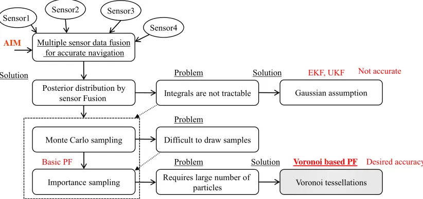
Desired accuracy
Solution
AIM Multiple sensor data fusion
for accurate navigation
Problem Posterior distribution by
sensor Fusion
Difficult to draw samples Monte Carlo sampling
Importance sampling
EKF, UKF Not accurate
Solution
Basic PF Problem Solution
Sensor2 Sensor3 Sensor1
Sensor4
Voronoi based PF
Problem
Requires large number of
[image:2.595.93.504.524.718.2]particles Voronoi tessellations Gaussian assumption Integrals are not tractable
eliminates particles with lower weights and multiplies particles with higher weights. Introducing resampling at every time step leads to sample impoverishment as simi- lar particles will be repeated number of times [12]. An ad-hoc approach called jittering was suggested to allevi- ate the sample impoverishment issue [17]. This approach added a small amount of Gaussian noise to each resam- pled particles so as to increase their diversity. However, this comes at the cost of immediately introducing some additional variance [12]. The performance of the SIS or SIR PF is limited because of the choice of the proposal distribution, especially when the likelihood is too narrow in comparison to the transition prior density function [4, 7,10].
To overcome these issues, a better proposal distribu- tion is desired, which is conditioned on the latest meas- urement [11-14]. Kalman based filters incorporate the latest measurement into the updated posterior state. Therefore, if EKF or UKF is used to generate the impor- tance distribution, latest measurement can be incorpo- rated into the distribution through the local linearization around each particle [15,16]. This is the principle behind the Extended particle filter (EPF) [15,18] and the Un- scented particle filter (UPF). The UPF is based on the UKF, an attractive alternative to EKF for highly non- linear problems. However, the computational cost per particle is higher as each particle is individually propa- gated through EKF or UKF to form the proposal distri- bution. To overcome these limitations, a hybrid extended particle filter (HEPF) was proposed [19]. HEPF com- bines the advantages of EKF (less computational load) and EPF (more accuracy during highly nonlinear regions) by alternating between the two filters, based on system dynamic. Another option to alternating between two dif- ferent filters is to marginalize out the linear states of the model from the nonlinear states as introduced in the Rao- Blackwellized particle filter (RBPF) [20,21]. In RBPF the linear states are estimated by the KF while the non- linear states by the PF portion of the algorithm. These strategies reduce the filter divergence issue and require less number of particles for outputting adequate naviga- tion solution. However, since the EPF or classic PF are still used by the HEPF or RBPF for the non-linear state estimation, their respective problems remain associated with the filter design [22].
Another approach to alleviate sample impoverishment problem in SIS/SIR filter is addressed by Pitt and Shepard in the form of the Auxiliary particle filter (APF) [23]. APF enhances the effectiveness of the importance sampling step by augmenting the existing good particles
1N s m
s
x
such that their predictive likelihood
11
density is a mixture of past states and the most recent observations. As long as the process noise is small, the performance of APF is superior to SIR PF. However, the moment the process noise increases, its accuracy decreases because of poor approximation of the
sm
p x .
Further, APF is computationally slower since the pro-
1
s m
x [21]
posal is used twice in the implementation. In likelihood PF (LPF), the likelihood function p z
x
is selectedto be the proposal density based o mption that particles drawn from the likelihood function will be closer to the true posterior density in comparison to par- ticles drawn from the state transition density [10,11]. This is effective only when the likelihood function is highly peaked and transition density is broad [21]. To combine the advantages of LPF and SIR filters, mixture particle filters (MPF) were developed. These MPF can be based on mixture posterior; where posterior is a weighted Gaussian mixture of parallel EKF or mixture proposal distributions [24], where distribution is based on mixture transition and likelihood functions. However, there are number of practical implementation limitations of these filters, for eg. the selection of Gaussian distribution pa- rameters or decision about the number of samples to be used from the transition and likelihood function etc.
From all these methodologies discussed in literatu m m
n the assu
re, co
3. Methodology of Voronoi Particle Filter
uple of prominent limitations like dispersion and sam- ple impoverishment, are being addressed by our method- ology. For a given finite set of generators, a Voronoi tessellation for each of these generators consists of all particles whose distance to a generator is not greater than to any other generator [25]. Motivated by this advantage of Voronoi tessellations, in this paper we have developed VPF method. In our methodology, Voronoi are created dynamically as and when new generators become avail- able.At previous epoch, N particles are generated from the
prior distribution p x
m1z1:m2
and assigned equal weights. Now each cles is passed through the developed system model as given by Equation (3).of these parti
(31 1, 1
m m m m
x x w )
where at time tm, xm
m0,1, 2,
is the state vectorof dimension r1, wm is the independent dynamic
noise r1 vector, and the nonlinear function m1
. ,of dimension r r , describes the state transitio
discrete time
n from
1
m to time m to get predicted state vec-
tor
ˆ 1 N s m s x
. The particles are now ready to be used for reation
N sm m
s
p z x
is high. Hence, the selected proposal
plained below.
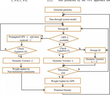
3.1. Situation I: GPS Data Is Available
These icles in storage , are subdivided into 3.1.1. Voronoi Gets Filled with the Maximum
Capacity
set of part
Ω
tessellations
k1 iV if k1 i
iV
and Vi Vji ,
i j, where ellation
lation Vˆi is constructed using a data point called
generator zi he Voronoi tessellation Vˆi for each zi is the set o all points closer to zi than
k is the num
. T
ber of tess s. Each such tessel
f zj for i j,
as defined by Equation (4).
ˆ Ω
Vi x xzi x zj fori1, 2, , , k i j
(4) Let denote a distance function induced by ano
,
d x z
rm that is equivalent to the l2 norm on N. Then
Voronoi tessellation of Ω, with respect to this tric, is defined by Equation (5).
me
ˆ Ω , ,
Vi x d x zi d x zj fori1, 2, , , k i j
(5)Dynamic creation of a Voronoi is withheld until G
the PS data is available, as GPS is the Voronoi generator
i
z (illustrated by Figure 2). Till the arrival of GPS, the oming INS particles are stored in Ω. Bythe time GPS data becomes available, storage Ω ight have none, some or huge set of INS particles. The decision to cluster an INS particle into the Voronoi is based on Equation (5). If the criterion is met, the INS particle joins with that Voronoi otherwise the INS particles are stored in Ω
inc
m
for the next Voronoi. This procedure is continued till the Voronoi gets the set number (N) of INS particles. With
this, Voronoi is closed and the algorithm looks for the dynamic creation of next Voronoi. Thus theVoronoi tes- sellations
k1i
V are formed such that particles with
similar we at satisfy Equation (5) are grouped to- gether in a tessellation Vˆi.
i
ights th
3.1.2. Voronoi Gets Partially Filled
ot satisfy Equation If sufficient number of particles did n
(5) then Voronoi gets partially filled. In this case, the data in storage Ω is redistributed depending on the dis- tance function uation (8)) and thus results in a dy- namic Voronoi. Given a tessellation
(Eq
N
V and a den-
sity function , defined in V, the mass centroid z of
V is defined by quation (6).
E
d d
v v
z
y y y
y y (6)In our case, the arithmetic mean (Equation (7)) corre- sp
onds to the mass centroid of V, where n is the number
of particles in the tessellation V
1 z z z z z z
z z
[image:4.595.336.505.80.386.2] z z z z GPS z GPS zz
Figure 2. Voronoi with center as z* = zGPS.
Given r rs,
here
a set of k particles which are gene ato
1, 2, ,
,
i
z
w i k
ˆ ,i
V we ca
; we can define their associated Vo- es-ronoi tessellations Vˆi. On the other hand, given the t
sellation n define their mass centroids zi as
illustrated by Figu . Here, we are interested in the situation where zi zi
re 2
, i.e., the particles zi, that se as generators for the Voronoi tessellations Vˆi are them-
selves the mass ds of those tessellations. We call such a tessellation Centroidal Voronoi tessellation [25].
Partially filled Voronoi has the generator zi and one can compute the mass centroid zi
for the data in storage
Ω
rve
centroi
. Now the process of simultaneously redistributing the particles in the storage Ω' and checking distance func- t (Equation (8)) between the new mass centroid and zi is iterated till convergence zi zi
is achieved. These
iterations guarantee that the Voronoi gets filled to the maximum capacity with zi
ion
i
z.
i, new
i,
d z z d z z (8)
Once the dynamic Voronoi is f
GPS measurement as the center z, weights
illed with the given
i
1
N s ms
w
of the particles are updated according to Equation (9) where
h is the measurement model.
s s X V
Z n X
(7)
1
s
ˆ N ˆ
s s s
m m m m m
The posterior density function (required den be represented by a collection of these predicted pa al
where b y
v and vbz denote the body frame velocities in
Y and Z directions respectively. The created Voronoi has all the particles with equal weights, which are later updated according to the new GPS center. The posterior density function (required density) will be represented by a collection of these predicted particles along with their updated weights.
sity) will rticles ong with their updated weight as given in Equation (10). The complete Voronoi based particle filter algorithm is illustrated in Figure 3.
ˆ N ˆ
1
s s
m m
p x z
wm xmxm (10)s
3.2. Situation II: GPS Data Is Unavail
data that is
e
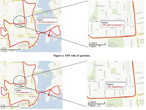
4. Results
able
The field test data was collected by installing various equipments in a test vehicle [24]. These include a Cross- bow IMU 300CC-100, reference high grade Honeywell IMU-HG1700, Novatel OEM GPS receivers and com- puter. The test trajectory covered a number of vehicle dynamics. Throughout the test, a minimum of seven sat- ellites were visible, except for several short natural GPS signal outages. For testing purposes, we carried out many experiments (without GPS outage) and here we report a couple of cases with N = 15 (Figure 5) and N = 45 parti- cles (Figure 6). We established the performance of the VPF algorithm by plotting the least square error (Figure 7) of the calculated trajectories (for N = 15 to 55) with respect to their reference solution. We also introduced several short GPS outages at various locations that are intentionally picked under diverse conditions. The posi- tion predicted by the VPF approach during one such In case of non-availability of GPS, the previous GPS
point acts as the starting point for zi. The INS data already collected is divided into arbitrary number of balls and their mass centroids zi
are computed. They then
follow a sequence of iterations to simultaneously correct the centers zi
and redistri ting the arbitrary balls with
reference to zi. The resulting balls are ordered in an
increasing e r threshold (i.e., z1
is more closer to
i
z
than z2
) and e Voronoi starts getting filled with the
first ball and incase it is not filled to its maximum capac- ity, second ball in row is used. This ensures creation of an appropriate Voronoi with propagated GPS (zi) as the center. Further, incorporation of the non-holonomic conditions, given by Equation (11) guarantees th vehicle progresses in the correct path.
0, 0,
b b
y z
v v (11)
bu
[image:5.595.112.481.399.718.2]rro th
Figure 4. VPF with 15 particles.
[image:6.595.62.539.88.257.2]Figure 5. VPF with 45 particles.
Figure 6. Least square errors vs particles.
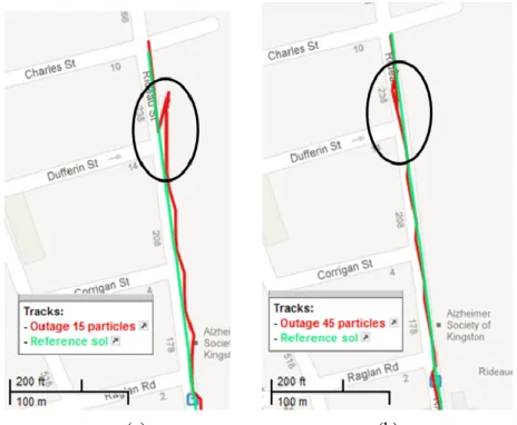
outage is compared with the reference differential GPS for N = 15 and N = 45 particles (Figure 7).
4.1. Without GPS Outage
In this section we demonstrate the successful completion of the 52 minute trajectory with as small as 15 particles
by our proposed Voronoi based particle filter. The tra- jectory data is shown using the GPS Visualizer toolbox. We observe that as the number of particles increases, the trajectory becomes smoother and smoother. Figures 4 and 5 illustrate the complete trajectories with N = 15 and N = 45 particles. We observe that trajectory with 45 par- ticles has lesser error and is smoother than the trajectory with 15 particles. We have highlighted a section of the
this observation. Figure 6 illus- ormance of the VPF with different number of particles ranging from 15 to 55. The least square error is calculated by comparing each trajectory with the ref- erence solution. We observe that as the number of parti- cles increases, the error decreases.
4.2. With GPS Outage
We carried out some initial experiments with GPS out- ages at various intentionally chosen locations. We could successfully bridge the GPS gap with as small as 15 par- ticles. This shows that our algorithm works in the GPS outage scenario as well. We report here the preliminarily trajectory to illustrate
(a) (b)
Figure 7. Performance of VPF with (a) 15 and (b) 45 parti- cles during GPS outage.
results for 15 and 45 particles as given in Figure 7, where GPS gap is highlighted. We can clearly see that the error with 45 particles (circled region in Figure 7(b)) is less than the error with 15 particles (circled region in Figure 7(a)). More work will be put in this scenario with longer GPS outages under diverse conditions in our fu- ture publications.
5. Conclusion
e havecation of the e concept of dynamic Vo- fall into the high like-
the VPF algorithm. Future work will include larger GPS outages at various
and this will be reported in later publication.
REFERENCES
[1] P. Misra and P. Enge, “Global Positioning System: Sig- nals, Measurements and Performance,” Ganga-Jamuna Press, Massachusetts, 2010.
[2] M. Grewal, L. Weill and A. Andrews, “Global Position- ing Systems Inertial Navigation, and Integration,” 2nd Edition, Wiley-Interscience, New Jersey, 2007.
doi:10.1002/0470099720
[3] N. El-Sheimy, “Inertial Techniques and INS/DGPS Inte- gration,” ENGO 623-Course Notes, University of Calgary, Calgary, 2006.
[4] P. Aggarwal, Z. Syed, A. Noureldin and N. El-Sheimy, “Integrated MEMS Based Navigation Systems,” Artech House, Norwood, 2010.
al, Z. Syed, X. Niu and N. El-Sheimy, “A Stan- dard Testing and Calibration Procedure for Low Cost
[7] B. Ristic, S. Arulampalan and N. Gordon, “Beyond the Kalman Filter: Particle Filters for Tracking Applications,” Artech House, 2004.
[8] S. Julier, J. Uhlmann and H. Durrant, “A New Approach for Nonlinear Transformations of Means and Covariances in Filters and Estimators,” IEEE Transactions on Auto- matic Control, Vol. 45, No. 3, 2000, pp. 477-482. doi:10.1109/9.847726
W developed a Voronoi based particle filter to integrate GPS and INS data for the navigation purpose. In some scenarios creation of Voronoi involves redistri- bution of the particles indicating the modifi
proposal distribution. Using th ronoi, we made more particles to
lihood region; thereby increasing the reliability of our proposed VPF algorithm. The robustness of the algo- rithm is illustrated by completing the whole trajectory with as minimum as fifteen particles with acceptable error. On increasing the number of particles to 45, we were able to achieve a smoother trajectory with less error compared to 15 particles case. Due to the redistribution principle, we are able to overcome the drawbacks of dis- persion (maximum number of particles ending up with negligible weights) and sample impoverishment (many identical particles found in the posterior distribution), inherent in conventional particle filters. In case of GPS outages, we incorporated non-holonomic constraints to create dynamic Voronoi with virtual GPS center. Based on this method, we have obtained initial results and demonstrated the performance of
locations in the trajectory
[5] P. Aggarw
MEMS Inertial Sensors and Units,” Journal of Naviga-tion, Vol. 61, No. 2, 2007, pp. 323-336.
[6] C. Hide, “Integration of GPS and Low-Cost INS Measu- rements,” Ph.D. Thesis, University of Nottingham, Not- tingham, 2003.
[9] N. Bergman, “Recursive Bayesian Estimation: Navigation and Tracking Applications,” Ph.D. Thesis, Linköping Uni- versity, Linköping, 1999.
[10] A. Doucet, N. Freitas and N. Gordon, “Sequential Monte Carlo Methods in Practice,” Springer, New York, 2001. [11] M. Arulampalam, S. Maskell, N. Gordon and T. Clapp,
“A Tutorial on Particle Filters for Online Nonlinear/Non- Gaussian Bayesian Tracking,” IEEE Transactions on Signal Processing, Vol. 50, No. 2, 2002, pp. 174-188. doi:10.1109/78.978374
[12] A. Doucet and A. Johansen, “A Tutorial on Particle Fil-tering and Smoothing: Fifteen Years Later,” In: D. Crisan and B. Rozovsky, Eds., Handbook of Nonlinear Filtering, Oxford University Press, Oxford, 2011.
[13] F. Gustafsson, F. Gunnarsson, N. Bergman, U. Forssell, J. Jansson, R. Karlsson and P. Nordlund, “Particle Filters for Positioning, Navigation and Tracking,” IEEE Trans- actions on Signal Processing, Vol. 50, No. 2, 2002, pp. 425-437. doi:10.1109/78.978396
[14] G. Kitagawa, “Monte Carlo Filter and Smoother for Non- Gaussian Nonlinear State Space Models,” Journal of Com- Graphical Statistics, Vol. 5, No. 1, 1996, putational and
pp. 1-25.
[15] R. Merwe, A. Doucet, J. Freitas and E. Wan, “The Un- scented Particle Filter,” University of Cambridge, Cam- bridge, 2000.
s, . 346-352.
sian Processes,” MITRE Technical Report, MTR 05W- 0000004, MITRE Corporation, 2005.
[17] N. Gordon, D. Salmond and A. Smith, “Novel Approach to Nonlinear and Non-Gaussian Bayesian State Estima- tion,” Proceedings of the IEEE, Vol. 140, 1993, pp. 107- 113.
[18] P. Aggarwal, D. Gu and N. El-Sheimy, “Extended Par- ticle Filter (EPF) for Land Vehicle Navigation Applica- tions,” International Global Navigation Satellite Systems (IGNSS), Sydney, 4-6 December 2007.
[19] P. Aggarwal, Z. Syed and N. El-Sheimy, “Hybrid Ex-tended Particle Filter for Integrated Navigation and Glob-al Positioning System,” Measurement Science and Tech- nology, Vol. 20, No. 5, 2009.
[20] A. Doucet, N. Freitas, K. Murphy and S. Russell, “Rao- Blackwellised Particle Filtering for Dynamic Bayesian Networks,” Proceedings of the 16th Conference on Un-certainty in Artificial Intelligence, Stanford, 30 June-3 July 2000, pp. 176-183.
[21] Z. Chen, “Bayesian Filtering: From Kalman Filters to
Particle Filters, and Beyond,” Adaptive Systems Labora-tory Technical Report, McMaster University,Hamilton. [22] Y. Jianjun, Z. Jianqiu and M. Klaas, “The Marginal Rao-
Blackwellized Particle Filter for Mixed Linear/Nonlinear State Space Models,” Chinese Journal of Aeronautic Vol. 20, No. 4, 2007, pp
doi:10.1016/S1000-9361(07)60054-5
[23] M. Pitt and N. Shephard, “Filtering via Simulation: Aux- iliary Particle Filters,” Journal of the American Statistical Association, Vol. 94, No. 446, 1999, pp. 590-599. doi:10.1080/01621459.1999.10474153
[24] J. Georgy, A. Noureldin, M. Korenberg and M. Bayoumi, “Low Cost 3-D Navigation Solution for RISS/GPS Inte-gration Using Mixture Particle Filter,” IEEE Transactions on Vehicular Technology, Vol. 59, No. 2, 2010, pp. 599- 615. doi:10.1109/TVT.2009.2034267
[25] Q. Du, V. Faber and M. Gunzburger, “Centroidal Voronoi Tesselations: Applications and Algorithms”, SIAM Re- view, Vol. 41, No. 4, 1999, pp. 637-676.