Multinuclear solid state NMR for the characterisation of inorganic materials

(1)

MULTINUCLEAR SOLID-STATE NMR FOR THE CHARACTERISATION OF INORGANIC MATERIALS

Valerie Ruth Seymour

A Thesis Submitted for the Degree of PhD at the

University of St Andrews

2013

Full metadata for this item is available in Research@StAndrews:FullText

at:

http://research-repository.st-andrews.ac.uk/

Please use this identifier to cite or link to this item:

http://hdl.handle.net/10023/3672

(2)

Multinuclear Solid-State NMR for the

Characterisation of Inorganic Materials

Valerie Ruth Seymour

This thesis is submitted in partial fulfilment for the degree of PhD

at the University of St Andrews

(3)

(4)

iii

Declaration

I, Valerie Ruth Seymour, hereby certify that this thesis, which is approximately 63000 words in length, has been written by me, that it is the record of work carried out by me and that it has not been submitted in any previous application for a higher degree.

I was admitted as a research student in September, 2008 and as a candidate for the degree of PhD in September, 2009; the higher study for which this is a record was carried out in the University of St Andrews between 2008 and 2012.

Date ……… Signature of candidate ………

I hereby certify that the candidate has fulfilled the conditions of the Resolution and Regulations appropriate for the degree of PhD in the University of St Andrews and that the candidate is qualified to submit this thesis in application for that degree.

(5)

iv

In submitting this thesis to the University of St Andrews I understand that I am giving permission for it to be made available for use in accordance with the regulations of the University Library for the time being in force, subject to any copyright vested in the work not being affected thereby. I also understand that the title and the abstract will be published, and that a copy of the work may be made and supplied to any bona fide library or research worker, that my thesis will be electronically accessible for personal or research use unless exempt by award of an embargo as requested below, and that the library has the right to migrate my thesis into new electronic forms as required to ensure continued access to the thesis. I have obtained any third-party copyright permissions that may be required in order to allow such access and migration, or have requested the appropriate embargo below.

The following is an agreed request by candidate and supervisor regarding the electronic publication of this thesis:

(i) Access to printed copy and electronic publication of thesis through the University of St Andrews.

Date ……… Signature of candidate ……

(6)

v

Abstract

In this work, multinuclear solid-state nuclear magnetic resonance (NMR) spectroscopy is used to investigate a range of inorganic materials, often in combination with DFT (density functional theory) studies. Solid-state NMR is particularly suited to the study of aluminophosphates (AlPOs), as the basic components of their frameworks have NMR active isotopes (27Al, 31P, 17O), as do many of the atoms that comprise the structure directing agent (13C, 1H, 15N), and the charge-balancing anions (OH−, F−). A study of the AlPO STA-15 (St Andrews microporous solid-15) provides an introduction to using solid-state NMR spectroscopy to investigate AlPOs. More in-depth studies of AlPO STA-2 (St Andrews microporous solid-2) and MgAPO STA-2 (magnesium-substituted AlPO) examine charge-balancing mechanisms in AlPO-based materials.

A range of scandium carboxylate metal-organic frameworks (MOFs), with rigid and flexible frameworks, have been characterised by multinuclear solid-state NMR spectroscopy (45Sc, 13C and 1H). The materials studied contain a variety of metal units and organic linkers. 13C and 1H magic-angle spinning (MAS) NMR were used to study the organic linker molecules and 45Sc MAS NMR was used to study the scandium environment in the MOFs Sc2BDC3 (BDC =

1,4-benzenedicarboxylate), MIL-53(Sc), MIL-88(Sc), MIL-100(Sc) and Sc-ABTC (ABTC = 3,3`,5,5`-azobenzenetetracarboxylate). Functionalised derivatives of Sc2BDC3 and MIL-53(Sc) were also studied. The 45Sc MAS NMR spectra are

found to be strongly dependant on the Sc3+ coordination environment.

27_{Al and}25_{Mg MAS NMR have been used to study Ti-bearing hibonite}

samples (of general formula Ca(Al, Ti, Mg)12O19), and results compared to a

recent complementary neutron powder diffraction study, in order to investigate the substitution sites for Ti3+/4+ and Mg2+. A DFT investigation was also carried out on the aluminium end member, CaAl12O19, due to debate in the literature on the 27_{Al NMR parameters for the trigonal-bipyramidal site. The substitution of Mg}

(7)

vi

Acknowledgements

My thanks go to my PhD supervisor Dr Sharon Ashbrook.

I would also like to thank various collaborators who provided the samples studied in this work: Professor Paul Wright and members of the Wright group - John Mowat, Eike Eschenroeder, Maria Castro, A. Lorena Picone and Zhongxia Han; and Dr Andrew Berry and Trish Doyle.

Thanks to past and present members of the Ashbrook group: Dr John Griffin, Martin Mitchell, Dr Karen Johnston, Dr Diego Carnevale, Daniel Dawson, Martin Peel and Scott Sneddon. Additional thanks go to Dr Dinu Iuga at the 850 MHz Solid-State NMR Facility, Warwick, Dr Julien Trébosc at the 800 MHz Facility, Lille, and Dr Herbert Fruchtl for computational assistance at the University of St Andrews. The UK 850 MHz solid-state NMR Facility used in this research was funded by EPSRC and BBSRC, as well as the University of Warwick including via part funding through Birmingham Science City Advanced Materials Projects 1 and 2 supported by Advantage West Midlands (AWM) and the European Regional Development Fund (ERDF).

(8)

vii

Chapter 1 Introduction

1.1 NMR of Inorganic Solids

1.1.1 Introduction

In solution-state nuclear magnetic resonance (NMR) spectroscopy automated instruments are widely used to for the routine acquisition of 1H and 13C spectra of organic molecules, even those as large as proteins (10 to > 100 kDa). Due to the anisotropic nature of interactions that provide information, in the solid state spectra result that are broadened, often over many 10s or 100s of kHz. For inorganic solids there is a range of nuclei that can be studied, many with their own challenging characteristics ranging from those with low   is the gyromagnetic

ratio, and therefore low sensitivity, and low natural abundance, to those with large quadrupolar couplings and long relaxation times. There is also less information on NMR parameters for many inorganic materials available in the literature, particularly for some less commonly studied nuclei, but it is a growing area of research.1,2,3 However, solid-state NMR is useful for examining a range of chemical and physical properties of a material, including the range of coordination environments present, substitution sites and hydration. Solid-state NMR spectra can be difficult to interpret and there has been an increased interest in the use of density functional theory (DFT) calculations to aid assignment and interpretation.4,5

(19)

2 1.1.2 Inorganic Materials

Microporous framework materials have widespread applications, such as catalysis, gas storage, purification and separation, and drug delivery.2 The term ‘microporous’ now includes groups of materials with compositions different to that of the original group to which it applied, namely aluminosilicate zeolites. One such group of microporous materials is the aluminophosphates (AlPOs), with frameworks that consist of corner sharing aluminate and phosphate tetrahedra and were first synthesised by Wilson et al. in the 1980s.6 Some AlPOs have similar topologies to zeolites, whereas others are new structures, and for some the AlPO form of a structure had been discovered prior to its zeolite equivalent. The neutral nature of AlPOs generally prevents inherent catalytic activity, but this can be generated by the inclusion of other atoms into the framework. For example, aluminium can be substituted by magnesium, and phosphorous by silicon to produce MgAPOs and SAPOs, respectively.7,8 Nevertheless, AlPOs themselves do have interesting structural aspects, and favorable adsorption properties.

AlPOs are typically synthesised using structure directing agents (SDAs), normally amines or quaternary alkylammonium ions. The term SDA is commonly used interchangeably with the term template, although the latter, strictly speaking, refers to when there is a close fit between the organic molecule and pore or cavity of the framework. The template (or SDA) is often charged when encapsulated within the framework, requiring charge-balancing ions to be present, typically F− or OH− ions. The location of these ions in the framework is of considerable structural interest and difficult to locate by diffraction. Usually the SDAs, and any charge-balancing anions, can be removed by calcination, heating to a high temperature to remove guest species, to give a, typically microporous, porous material.

(20)

3

flexible route to design materials, particularly porous frameworks, for a variety of applications, with predesigned building units. Metal carboxylate MOFs can contain linkers that are di-, tri- or tetra- carboxylates.9 The structures may also contain bridging hydroxyls or oxygen atoms (such as μ3O, an oxo ligand shared

between three cations at the centre of a cluster), or terminal hydroxyls or water. The MOFs can be modified, in the case of phenyl carboxylates by introducing substituents onto the aromatic ring, either by preparing with modified linkers or by postsynthetic modification to tune the properties of the MOF.10

Hibonite, calcium hexaluminate (CaAl12O19), is the Al pure end member

of a range of solid solutions with the magnetoplumbite-type structure (AB12X19).

Hibonite materials, containing various substitutions such as Fe and Ti, are found in terrestrial deposits and meteorites and are being studied to gain insight into solar systems, by examining the mineralogy of astronomical environments.11 Hibonite has the potential to act as an oxybarometer to study the redox states of meteoric rock, and therefore the history of the rock.12 Synthetic hibonite is used in tough ceramic composites, with significant effect on the physical and thermal properties.13,14 The structure of hibonite consists of alternating layers of spinel blocks (S) and hexagonal blocks (R), in the sequence RSR`S`, where R` and S` are rotated 180° relative to the respective R and S blocks.15 Hexaluminates such as CaAl12O19 and SrAl12O19 have been widely studied by X-ray diffraction and

high-resolution 27Al NMR, due to their unusual structure.16

1.1.3 Applicability of NMR to the Study of Inorganic Solids

(21)

4

The basic elements found in hibonite are NMR active (43Ca, 27Al, 17O), although these vary greatly in their accessibility and ease of study.

The templates used in AlPO synthesis and the organic linkers of MOF predominately contain 13C and 1H nuclei, which are readily studied by NMR providing the requisite line narrowing techniques are applied. 13C NMR is used to determine whether the template or linker has been encapsulated or incorporated, respectively, intact. The low natural abundance of 13C is overcome by the routine use of cross polarization (Chapter 3). 1H NMR spectra can give information not just on the template or linker, but also on the incorporation of water or hydroxyls. This might be in the form of a water molecule or hydroxyl group coordinated to the structure, structural acid protons, surface adsorbed species or water molecules in the pores of framework materials. The use of 1H NMR in the solid state is hampered by strong dipolar broadening, often requiring ultra-fast MAS rates (see Section 3.2.1). A further nuclide found in templates and linkers is nitrogen, which has two NMR active isotopes 14N and 15N, of which 15N (I = 1/2) is more amenable to study in the solid state, than the quadrupolar (I = 1) isotope, despite a lower natural abundance (15N 0.35%, 14N 99.64%). 14N typically requires a time consuming and inefficient stepped frequency approach to obtain solid-state NMR spectra or alternatively, indirect acquisition in a two-dimensional experiment.

31_{P (I = 1/2), a framework species in AlPOs, has 100% natural abundance.}

Phosphorous shifts are sensitive to the local environment, including bond lengths and bond angles, and the coordination number.1 It has been observed that 31P resonances experience a shift due to coordination of hydroxyls to neighbouring Al.17,18 31P NMR can therefore be used to study the dehydration/hydration of AlPOs. The 31P chemical shift is also sensitive to next-nearest neighbour substitutions, and can, therefore, be used to examine substitution of non-paramagnetic metal cations into AlPOs.19 It can also provide an indication of whether the substitution occurs randomly or is ordered throughout the material.20

29_{Si, a framework species of zeolites and a possible substituent for AlPOs, also}

(22)

5

27_{Al has 100% natural abundance, and has been extensively studied.}1,22 _It

is present in a wide range of inorganic materials, including all three examples discussed in Section 1.1.2. The 27Al chemical shift is strongly dependent on the coordination geometry and neighbouring atoms. For example, four-, five- and six-fold coordinate Al can be identified for as-prepared AlPOs, where extra-coordinated water, hydroxyls or fluoride may increase the coordination number of the nominally tetrahedral Al. Removal of these species by calcination gives AlO4,

which is readily observed, as are the effects of rehydration. The 27Al quadrupolar coupling is also sensitive to the coordination number and local geometry. Whilst

27_{Al is quadrupolar (I = 5/2), experimental methods such as MQMAS}

(multiple-quantum MAS, discussed in Chapter 3) enable high-resolution spectra to be acquired, distinct species resolved and information to be obtained. In many cases, MQMAS can resolve resonances for cystallographically-distinct sites that have the same coordination number. There have been fewer studies using 45Sc (I = 7/2) NMR but the same methodology typically used for 27Al can be applied, and it has been shown to be a sensitive probe of the local environment of inorganic solids, including framework structures.23Magnesium can be substituted for aluminium in AlPOs and hibonite materials, but 25Mg has a relatively low  and only 10% natural abundance, often requiring the use of additional sensitivity enhancement techniques.

The study of 17O, whilst quadrupolar (I = 5/2) and of low natural abundance (0.037%), is becoming increasingly popular with access to high magnetic fields, fast MAS rates and improved isotopic enrichment procedures.24,25

(23)

6

1.2 Thesis Overview

This thesis is concerned with the solid-state NMR investigation of a range of inorganic materials, specifically aluminophosphates, scandium-containing metal-organic frameworks and Ti-bearing hibonite materials. An introduction to these materials was given in Section 1.1.2 and the applicability of NMR for their study in Section 1.1.3. Chapter 2 provides a background to NMR spectroscopy introducing some basic principles and a description of the interactions present. Chapter 3 provides general experimental NMR details and discusses a range of experimental methods, and general computational details for the DFT calculations also utilised extensively in this work.

The results and discussion of the materials studied are presented in Chapters 4 to 6. Chapter 4 presents work on the first class of inorganic materials, aluminophosphates, with the investigation of two different AlPOs, namely STA-15 (St Andrews-STA-15), a novel large pore aluminophosphate, and STA-2 (St-Andrews-2), a member of the ABC-6 family of zeotypes. In the as-prepared materials for both AlPOs, hydroxyls are required to charge balance the encapsulated template. The MgAPO form of STA-2 has also been the subject of study, where the incorporation of Mg2+ into the framework provides an alternative charge-balancing mechanism in the as-prepared material. Chapter 5 is concerned with a different group of framework materials, scandium metal-organic frameworks (MOFs), which exhibit both rigid and flexible frameworks. The Sc MOFs studied have carboxylate linkers, with varying ScO6 coordination

environments, such as isolated octahedra, corner-sharing chains or trimers. For two of these MOFs, Sc2(BDC)3 and MIL-53, a series of compounds with modified

linkers was also studied. Chapter 6 presents the investigation of a series of synthetic Ti-bearing hibonite materials, with the general formula Ca(Al, Ti, Mg)12O19, to study the substitution sites of Ti and Mg. The synthetic Ti-bearing

(24)

7

compared with results from neutron powder diffraction. Supplementary information is provided in the Appendices and accompanying CD.

1.3 References

1. K. J. D. Mackenzie and M. E. Smith, in “Multinuclear Solid-State NMR of Inorganic Materials”, Pergamon, Oxford, 2002.

2. P.A. Wright, in “Microporous Framework Solids”, RSC Publishing, Cambridge, 2008.

3. J. V. Hanna and M. E. Smith, Solid State Nucl. Magn. Reson., 38, 1, 2010. 4. S. E. Ashbrook, M. Cutajar, C. J. Pickard, R. I. Walton and S. Wimperis,

Phys. Chem. Chem. Phys., 10, 5754, 2008.

5. T. Charpentier, Solid State Nucl. Magn. Reson., 40, 1, 2011.

6. S. T. Wilson, B. M. Lok, A. Messina, T. R. Cannan and E. M. Flanigen, J. Am. Chem. Soc., 104, 1146, 1982.

7. S. T. Wilson and E. M. Flanigen, ACS Symp. Series, 398, 329, 1989.

8. B. M. Lok, C. A. Messina, R. L. Patton, R. T. Gajek, T. R. Cannan and E. M. Flanigen, J. Am. Chem. Soc., 106, 6092 1984.

9. O. M. Yaghi, M. O’Keeffe, N. W. Ockwig, H. K. Chae, M. Eddaoudi and J. Kim, Nature, 423, 705, 2003.

10.T. Devic, P. Horcajada, C. Serre, F. Salles, G. Maurin, B. Moulin, D. Heurtaux, G. Clet, A. Vimont, J-M. Grenèche, B. Le Ouay, F. Moreau, E. Magnier, Y. Filinchuk, J. Marrot, J-C. Lavalley, M. Daturi and G. Férey, J. Am. Chem. Soc., 132, 1127, 2010, and references therein.

11.A. M. Hofmeister, B. Wopenka and A. J. Locock, Geochim. Cosmochim. Acta, 68, 4485, 2004.

12.P. M. Doyle, P. F. Schofield, A. J. Berry, A. M. Walker and K. S. Knight, in preparation, 2012.

13.L. An, H.-C. Ha and H. M. Chan, J. Am. Ceram. Soc., 81, 3321, 1998. 14.D. Asmi and I. M. Low, Ceram. Int., 34, 311, 2008.

(25)

8

16.L.-S. Du and J. F. Stebbins, J. Phys. Chem. B, 108, 3681, 2004, and references therein.

17.D. Akporiaye and M. Stocker, Zeolites, 12, 351, 1992.

18.A. Tuel, C. Lorentz, V. Gramlich and Ch. Baerlocher, C. R. Chim., 8, 531, 2005.

19.G. Mali, A Ristić and V. Kaučič, J. Phys. Chem. B, 109, 10711, 2005. 20.P. J. Barrie and J. Klinowski, J. Phys. Chem., 93, 5974, 1989.

21.R. Oestrike, W.H. Yang, R. J. Kirkpatrick, R. L. Hervig, A. Navrotsky, B. Montez, Geochim. Cosmochim. Acta, 51, 2199, 1987.

22.M. Haouas, C. Martineau and F. Taulelle, “NMR of Quadrupolar Nuclei in Solid Materials” in Encyclopedia of Magnetic Resonance, Eds-in-chief R. K. Harris and R. E. Wasylishen, John Wiley, Chichester. Published online 15th Dec 2011.

23.A. J. Rossini and R. W. Schurko, J. Am. Chem. Soc., 128, 10391, 2006.

24.J. M. Griffin, L. Clark, V. R. Seymour, D. W. Aldous, D. M. Dawson, D. Iuga, R. E. Morris and S. E. Ashbrook, Chem. Sci., 3, 2293, 2012.

25.S. E. Ashbrook and M. E. Smith, “Oxygen-17 NMR of Inorganic Materials” in Encyclopedia of Magnetic Resonance, Eds-in-chief R. K. Harris and R. E. Wasylishen, John Wiley, Chichester. Published online 15th Dec 2011.

(26)

9

Chapter 2 Background

This thesis is concerned with the application of solid-state NMR spectroscopy to study a range of inorganic solids. NMR is a well-established characterization technique and a fundamental tool for chemical analysis. It can be used to examine local structure, disorder and dynamics, in a highly selective, element specific and sensitive way. It is complementary to other characterization techniques commonly used for studying solids, such as X-ray diffraction (XRD). The basic principles of NMR are introduced in this chapter.

2.1 NMR Theory

2.1.1 Nuclear Magnetism

Spin, I, is the intrinsic angular momentum of atomic nuclei. The magnitude of the spin angular momentum is given by

| | [ ( )] , (2.1)

where I is the corresponding spin quantum number and can be zero, an integer or half integer number (I = 0, / , , 3/ , …), and is the reduced Planck’s constant. I must be greater than 0 for a spin to be considered NMR active. A second quantum number, mI, the magnetic quantum number, has 2I + 1 values,

which range from to − . This defines the orientation of I when projected onto an arbitrary axis, usually the z-axis,

m . (2.2)

(27)

10

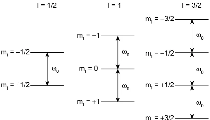
Figure 2.1: The effect of the Zeeman interaction on the energy levels for spin I = 1/2, 1 and 3/2 nuclei.

 ,

z z  I

 , (2.3)

where is the gyromagnetic ratio and z is the z component of .

In the absence of an external magnetic field the 2I + 1 spin states are degenerate in energy. This is lifted when a magnetic field, B0, is applied, by the

Zeeman interaction, and is shown in Figure 2.1 for spin I = 1/2, 1 and 3/2 nuclei. If the applied field is defined as along the z-axis, then the energies of the states are given by

|m⟩  m . (2.4)

The quantum selection rule is ∆mI = ±1 for an observable transition, resulting in

transitions with a frequency given by

, (2.5)

[image:27.595.106.462.69.273.2]

(28)

11

used, typically 2-22 T. Hence, radiofrequency radiation, rf, is used to induce NMR transitions.

When a macroscopic sample is placed in a magnetic field the nuclei distribute among the energy levels according to the Boltzmann distribution. The population difference induces a bulk magnetization which may be represented by a vector M, aligned with the field. Due to small differences sensitivity is an issue in NMR spectroscopy. For a given field strength, M is larger for high- nuclei, and for a given nucleus the magnitude of M will increase with field strength.

2.1.2 The Vector Model

The classical vector model1 can be used to describe nuclear spin systems during a pulsed NMR experiment. Whilst it is only really suitable for uncoupled spin I = 1/2 nuclei it provides a starting point for examining basic ideas such as the effect of an rf pulse and the subsequent spectral acquisition. The model considers the bulk (net) magnetization M of the sample, which can be represented as a vector aligned with the magnetic field B0. The z-axis of the laboratory frame

is set as the direction of the applied field, as shown in Figure 2.2(a). A short pulse

of oscillating rf radiation, with frequency rf, is applied, which interacts with nuclei in the sample. It is now more convenient to consider a rotating frame, i.e.,

rotating at a frequency rf around B0 in this frame. The effect of the rf pulse is that

the bulk magnetization is tilted away from the z-axis [Figure 2.2(b)]. When at such an angle the magnetization precesses about the field, at frequency 0. The

effect of an applied pulse of strength B1 is defined by a flip angle , through

which the magnetization vector nutates,

 , (2.6)

where p is the duration of the pulse. The magnetization vector then precesses

around the effective field in this frame at a frequency [Figure 2.2(c)],

  _rf . (2.7)

(29)

12

Figure 2.2: Vector model representation of (a) net magnetization vector of the spin system, at thermal equilibrium, along the z-axis, (b) vector rotates away from z-axis about the direction of the applied rf pulse of strength B1, through a flip angle , and (c) free precession and relaxation,

results in the FID.

The precession of the magnetization vector induces a current in a coil placed in the xy plane, which is amplified and recorded. This signal decays over time, through relaxation processes, and is termed the free induction decay (FID).

2.1.3 Relaxation

The bulk magnetization returns over time to its equilibrium position. The return of the z-component of magnetization to its equilibrium value (longitudinal relaxation) is characterised by an exponential time constant T1. The time constant

T2 describes the transverse relaxation, due to the decay of magnetization in the xy

plane. Typically, in solids, the T1 relaxation time is greater than T2, with the

sample dependent T1 on the order of ms to hours, and T2 on the order of 10 to

1000 ms. In contrast, in solution T1 is typically a few ms. T1 determines the rate at

which experiments can be repeated and therefore the acquisition of solid-state NMR spectra can be time consuming. However, the values are reasonably short for the majority of the nuclei studied in this thesis.

2.1.4 Fourier Transform

(30)

13

Figure 2.3: Schematic representation of data converted from the time domain to the frequency domain using a Fourier transform.

from the time domain to the frequency domain [Figure 2.3], using a Fourier transformation (FT)3

( ) ∫s(t)e (i t)dt . (2.8)

Quadrature detection involves the measurement of two separate components of the FID in order to produce a complex NMR signal that distinguishes the sign of the resonance offset, , so that FT produces an unambiguous spectrum. Two detectors orthogonal to each other in the rotating frame are used, leading to the acquisition of two signals, which are 90° out of phase with each other. One is a cosine function and the other a sine function of the offset frequency. The two components are considered as real and imaginary components of a single complex signal.

An FID is usually the sum of many oscillating waves of differing frequencies, amplitudes and phases. The general form of the time-domain signal contains cosine and sine functions of the offset frequency Ω, decaying with a rate proportional to 1/T2 [Equation 2.9]. The conversion to the frequency domain

(31)

14

Figure 2.4: One-dimensional (a) absorptive (real) and (b) dispersive (imaginary) lineshapes.

( ) [cost i sint]e ( t/T )

( ) ( ) i (∆ )

( ) ₍ /T

/T ) ( )

( ) ₍ ( )

/T ) ( )

(2.9)

(2.10)

(2.11)

(2.12)

2.1.5 Density Operator Formalism

The density operator formalism4 is a more rigorous approach for describing NMR experiments than the simple vector model, and a useful tool for examining multiple pulse experiments and higher-order spin systems. A macroscopic sample contains a collection of spin systems, each of which may be

represented by a wavefunction (t), that can be described as a linear combination of elements of an orthogonal basis set | ⟩, as shown in Equation 2.13, where ci(t)

are time-dependent coefficients

(32)

15

In the density operator approach the elements, i,j(t), of the corresponding density matrix are the products of the expansion coefficients of the wavefunction,



_i,(t) ⟨i|(t)|⟩ ci(t)c(t) , (2.14)

where the overbar denotes an ensemble average and * a complex conjugate. The evolution of the density operator over time is given by the Liouville-von Neumann equation,

 

_i

_

_H

_{   }

_t _, _t

_

dt t

d _ _ _,

(2.15)

where H is the time-dependent Hamiltonian for the system, which can be solved (if H is time-independent or can be made so by transforming to a different reference frame) to give:

(t) e ( i t)( )e (i t) , (2.16)

where (0) is the density operator at time zero. Simulation programs such as SIMPSON,5 which are used later in this work, use this formalism to consider the effects of pulses and delays within an NMR experiment.

2.1.6 Coherence

If we consider an ensemble of non-interacting spins, each described by a superposition of states, i.e., corresponding to the two Zeeman levels for a spin I =

1/2 nucleus,  and  , the complex superposition coefficients,c_

 

t and c_

 

t ,

which describe the contribution to these states, have phases _ and _

respectively, at t = 0. The wavefunction is therefore

(33)

16 The density matrix then has the form

(t) ( c cc e i( )

c_c_e i(  ) c_

) . (2.18)

The diagonal elements _c2

 and c2 refer to the populations of the  and 

states, respectively. If the off-diagonal elements have the same relative phases for each spin then they have non-zero magnetization and are said to have phase coherence. Coherence is generated by individual spins in the sample experiencing the same interaction with the applied rf field.

A pulse results in the rotation of the axis along which polarization is aligned. f an o erator acquires a hase of − from a z-rotation through angle

it has coherence order . As such, the coherence order can only be changed by a pulse. A coherence order of = 0 corresponds to either zero-quantum or

z-magnetization, = are single quantum, and  = > 1 are multiple quantum coherences.6

The coherence order needs to be controlled during a pulse sequence and a coherence transfer pathway diagram shows the desired coherence during each free precession interval. The coherence transfer pathway starts at  = 0, i.e., at thermal

equilibrium, and when quadrature detection is used,2finishes at  − . Multi

le-quantum (MQ) coherences (23 etc. are not directly observable, but are used in the more complex NMR experiments utilised in this thesis.

2.1.7 Product Operator Formalism

It quickly becomes too complicated to use the density operator approach to deal with nuclei with high spin quantum number. A more convenient approach is to expand the density operator as a linear combination of a basis set of operators. For a single spin (I = 1/2) the density operator can be expressed as a linear combination of the operators Ix, Iy and Iz, which represent the x-, y- and

(34)

17

 

t  aIxbIycIz

 , (2.19)

where a, b, and c are numbers related to the proportion of magnetization. For a coupled two-spin system 16 product operators can be formed from the combinations of the operators for spin 1 and spin 2.

The evolution of the density operator can be expressed as6

(t) cos t sin t . (2.20)

A is the original operator and C the new operator, and B is the transformation (flip angle, free precession) for time t. The effect of an on resonance rf pulse along x, for a duration p and using field strength 1, is shown by the following example

(t) cos ysin , (2.21)

where A = Iz and C = Iy, with B = 1. The transformation of product operators is

often shown with “arrow notation”, with that for Equation 2.21 given as

→ cos ysin . (2.22)

For standard pulses this can be simplified, as 1 p is simply the pulse flip angle ,

so, for example, for a 90x pulse

→ cos ysin ,

→ _y .

(2.23)

Likewise, the effect of free precession after the pulse is

(t) _ycost sint ,

y t

→ ycost sint ,

(35)

18

with the operators A = −Iy and C = Ix, and B = . The subsequent identities for

pulses, chemical shift evolution and scalar coupling, can be used to follow multiple-pulse experiments, without the need for complicated maths.

2.1.8 Two-Dimensional NMR

Two-dimensional experiments can be used to obtain further detail than provided by one-dimensional spectra, including for example, information on through-bond or through-space connectivities of Al to P in AlPOs. In general, 2D NMR experiments contain a preparation, evolution, and mixing or conversion steps prior to acquisition. The preparation step creates the magnetization, then, after evolving for time t1, a combination of pulses is used to transfer the

magnetization between spins (mixing step). The FID is then acquired during t2

and its amplitude is modulated by the evolution in t1. Two-dimensional data sets

are obtained by the incrementation of the t1 evolution period. Fourier

transformation is applied in both dimensions [Equation 2.25], and the FT spectrum shows between which spins the magnetization was transferred. Different sets of pulses can be used for preparation and conversion, producing transfer through different mechanisms (e.g., transfer through dipolar coupling or J-coupling).

(t ,t ) T along t→ (t , ) T along t→ ( , ) (2.25)

The real and imaginary components of the 2D spectrum contain absorptive and dispersive components. This gives phase twisted lineshapes, which are undesirable. Hypercomplex FT can be used to obtain pure absorption mode 2D lineshapes, but with the disadvantage that there is a lack of frequency discrimination in the 1 dimension. Two data acquisition and processing schemes commonly used to distinguish frequencies are States, Haberkorn and Ruben8 and TPPI9 (time-proportional phase incrementation). The States approach involves the acquisition of two datasets per t1 increment, where the phase of the preparation

(36)

19

combination of the two datasets. In an alternative approach, TPPI, sign discrimination is restored by incrementing the phase of the first pulse by 90° for each t1 increment, and halving the t1 increment, so only one dataset is acquired for

each t1 increment.

2.2 Solid-State NMR

Solid-state NMR spectra can contain a vast amount of information owing to various interactions that affect them, and as a result they can be hard to interpret. Therefore, various techniques are used to remove different interactions thereby improving sensitivity or resolution to enable information to be extracted more easily [Chapter 3]. More complex approaches can be used to reintroduce or use specific interactions in a controlled manner, thereby obtaining site specific information on local geometry or disorder.

2.2.1 Internal Interactions

The interaction of nuclei with an external field is the basis of NMR spectroscopy, with this Zeeman interaction generally dominant. However, nuclei experience other magnetic and electric fields, arising internally from the arrangement of atoms and nuclei, which provide detail about the local environment. These internal interactions include chemical shielding, dipolar coupling, quadrupolar coupling and scalar couplings. Information on these interactions is encoded within the NMR spectrum, in the form of shifts, broadenings and lineshape changes.

(37)

20

Figure 2.5: Schematic representation of the relationship of (a) the laboratory frame and (b) the principal axis system (PAS). The interaction tensor is represented as an ellipsoid, and the principal axes of the ellipsoid coincide with the interaction principal values.

2.2.2 Chemical Shielding Anisotropy

The magnetic field experienced by a nucleus typically differs from the applied external magnetic field owing to the presence of local fields, which oppose or augment the applied field. These are generated by the motion of the

local electrons within their orbitals. The perturbed Larmor frequency, '

0, is given

by

( ) , (2.26)

where  is a shielding parameter. Hence, the NMR frequency for a particular spin

depends not just upon and B0, but also on the chemical environment.

It is more convenient to define a chemical shift, a deshielding

parameter, rather than the absolute shielding  which is difficult to measure. ,

usually quoted in parts per million (ppm),is defined in Equation 2.27 in terms of

the difference between the resonance frequencies of the nucleus of interest ( )

and a reference frequency ( ref)10





ref ref 6

10 

 . (2.27)

The two parameters  and  are related by Equation 2.28, where an approximation

(38)

21

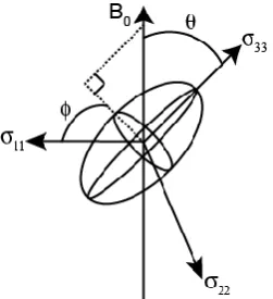
Figure 2.6: Schematic representation of the shielding tensor, with the three principal components of the PAS defined as 11, 22 and 33. The angles  and  define the orientation of the tensor

relative to B0.















 



  

 6 ref

ref ref

6 ₁₀

1 10

. (2.28)

Chemical shielding anisotropy (CSA) arises because the shielding of a nucleus (i.e., the surrounding electron density) is rarely spherical, but is orientationally de endant, or “anisotro ic”, i.e., it varies with the orientation with respect to the direction of the applied magnetic field, B0. For liquids, the rapid

tumbling motion means that an average, or isotropic, shift is observed. However, for solids this anisotropy is important, as there is typically no motion on the same timescale.

In the principal axis system (PAS) the shielding tensor, , can be described by an ellipsoid, due to its diagonal matrix form and the tensor

 ₍ 



₃₃) , (2.29)

where 11, 22 and 33 are defined as the three principal components of the tensor,

as shown in Figure 2.6. Correspondingly, 11, 22 and 33 are the principal values

of the chemical shift tensor. Using the convention |33 − iso| ≥ |11 − iso| ≥ |22 −

iso|,11 the shielding parameter can be parameterised by three values, iso, cs and

[image:38.595.250.376.72.210.2]

(39)

22

_iso ( /3)(  ₃₃) . (2.30)

The chemical shielding anisotropy, cs, is

_cs (₃₃ _iso) , (2.31)

and the asymmetry, cs, where 0 < cs < 1 is

_cs ( )/(₃₃ _iso) . (2.32)

There are different conventions in use in the literature.

The observed chemical shift of a resonance is shown in Equation 2.33. The first term, in the laboratory frame, is isotropic and the second term is anisotropic12

 iso ( cs/ )[(3 cos  ) _cs(sin cos )] , (2.33)

where and  are the angles that define the orientation of the tensor relative to the external magnetic field B0 [Figure 2.6]. So for each orientation of the shielding

tensor a different chemical shift is observed. A powdered sample contains many single crystals, which will have different orientations relative to B0, and therefore

different chemical shifts are observed. Consequently, a broad powder-pattern

(40)

23

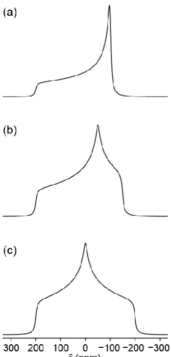
Figure 2.7: Simulated (using SIMPSON) static powder pattern lineshapes (B0 = 14.1 T) for a spin

I = 1/2 nucleus with cs = 200 ppm and asymmetry, cs of (a) 0, (b) 0.5 and (c) 1.

2.2.3 Dipolar Coupling

The magnetic moment of a nucleus interacts with those arising from nearby nuclei through space, in an interaction termed the dipolar coupling. For liquids this interaction is averaged to zero as a result of the rapid tumbling motion, i.e., the isotropic value of the coupling is zero. In solids the dipolar coupling is a major source of broadening. This interaction can be inter- or intra-molecular, and homo- or hetero-nuclear. The interaction is dependent on the gyromagnetic ratio, , of the two spins involved, the distance between them, r, and the

[image:40.595.227.395.67.417.2]

(41)

24

₍_{3 cos}_ ₎

where

₍

)r3 .

(2.34)

In Equation 2.34, DPAS_{is the dipolar-coupling constant in the PAS,}__{is the angle}

describing the orientation of the internuclear vector with respect to the magnetic field.

The effect of dipolar coupling on the spectrum (for a spin I = 1/2 nucleus) is that each single transition is split into a doublet separated by 2 D (heteronuclear

I = S = 1/2 spin system) or 3 D (homonuclear I = S = 1/2 spin system). The dipolar interaction, in a similar manner to the CSA, is orientationally dependent, therefore the dipolar splitting depends on the angle between the internuclear vector and the magnetic field. Variation of the angle in a powdered solid, results in a “ ake-doublet” linesha e, as shown in Figure 2.8(a). In reality it is rare to find two isolated spins, and therefore there are many dipolar couplings between numerous spins. Lineshapes therefore typically exhibit Gausssian broadening, as shown in Figure 2.8(b). Simulated spectra showing the effect of different amounts of Gaussian broadening, on the appearance of a 27Al NMR lineshape, are shown in

(42)

25

Figure 2.8: Schematic spectra, simulated using SIMPSON, of a spin I = 1/2 nucleus with (a) dipolar coupling (of 5 kHz) to a S = 1/2 nucleus and (b) subject to many different couplings to a range of different nuclear species. The lineshape in (a) is a Pake doublet and in (b) a Gaussian-like lineshape resulting from many dipolar couplings.

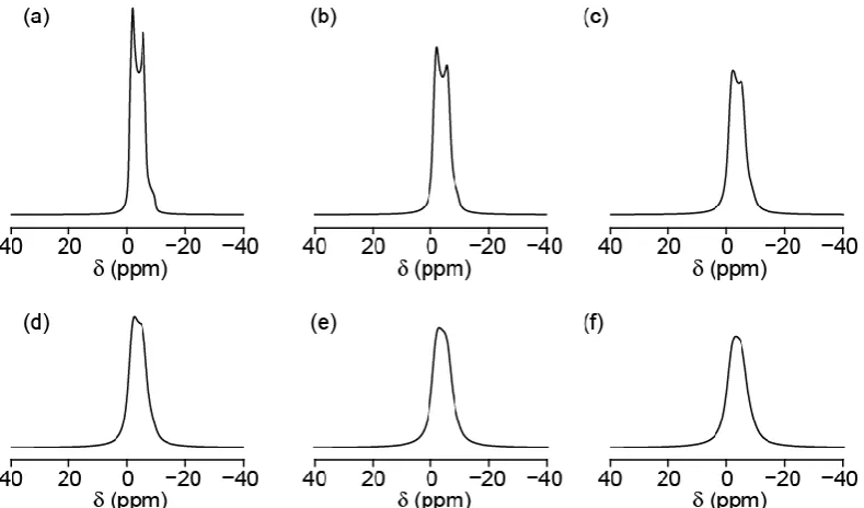
Figure 2.9: Simulated spectra (using SIMPSON) for 27_{Al (I = 5/2), with B}

0 = 14.1 T, CQ = 4 MHz,

Q = 0, 10 kHz MAS rate. Linebroadening of (a) 100, (b) 200, (c)300, (d) 400, (e) 500 and (f) 600

Hz. The NMR parameters CQ and Q will be discussed in Section 2.2.4 and MAS in Chapter 3.

2.2.4 Quadrupolar Coupling

Quadrupolar coupling needs to be considered for nuclei with I > 1/2 (e.g.,

27_Al,45_{Sc etc.). The electric quadrupole moment (EQM) of these quadrupolar}

[image:42.595.114.509.324.556.2]

(43)

26

nucleus, while the EFG is present in solids owing to the distribution of other nuclei and electrons nearby, for nuclei not at sites of cubic symmetry. The magnitude of the EQM and of the EFG affect the strength of the interaction. The spectra of quadrupolar nuclei can potentially give information on coordination number, symmetry and distortions, if this interaction can be accurately measured.

The quadrupolar coupling, in the PAS (in rad s 1) is given by Equation 2.35, and the quadrupolar splitting parameter, in the laboratory frame, to a

first-order approximation  1

Q in Equation 2.36

3

( )

( ) ₍_{3 cos} _ _ _sin __cos_₎

(2.35)

(2.36)

where the quadrupolar coupling constant, CQ, and the quadrupolar asymmetry

parameter, Q, are defined in Equations 2.37 to 2.39. The EFG can be described by a tensor with principal values Vxx, Vyy, and Vzz, which are assigned, by

convention, as |Vzz| ≥ |Vxx| ≥ |Vyy|. Two parameters, CQ and Q, are used to specify

the EFG of a nucleus I. The largest principal value of the EFG, i.e., Vzz is equal to

eq [Equation 2.37]. In Equation 2.39 Q is the nuclear quadrupole moment and e is the magnitude of the electric charge. The orientation of the interaction tensor with

respect to the laboratory frame is described by the angles  and .

eq zz yy xx Q V V V 

 ≤ Q≤ 1

e q h e V h (2.37) (2.38) (2.39)

The effect of the quadrupolar interaction on the Zeeman energy levels of a half-integer quadrupolar nucleus is to produce two types of transitions; (i) the central transition (CT) and (ii) pairs of satellite transitions (ST). As shown in

(44)

[image:44.595.150.479.70.412.2]

27

Figure 2.10: Energy levels for a spin I = 5/2 nucleus. The CT is unaffected to first order, unlike the STs. Both types of transitions are affected to second order.

approximation of the perturbation of the energy levels, unlike the ST, which exhibit a variation in the frequency of the corresponding transitions. Consequently, NMR experiments in the solid state generally focus only on the relatively narrow CT.

When the quadrupolar interaction is large, and the first-order approximation is not sufficient to describe the effect of the interaction upon the energy levels, a more complex second-order correction needs to be taken into account. This interaction now affects all transitions [Figure 2.10] and the CT now displays an anisotropically broadened lineshape. This second-order interaction is inversely proportional to the external magnetic field.

The second-order contribution for a general symmetric transition

I

I m

m E

E (e.g., 1Q, 3Q and 5Q) for a nucleus of general spin quantum

(45)

28









 

















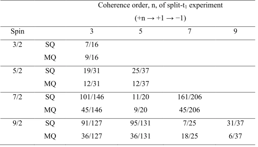
_               Q 4 I 4 Q 2 I 2 Q 0 I 0 0 2 PAS Q ) 2 ( m ) 2 ( m , , , Q m , I A , , , Q m , I A Q m , I A E E I I (2.40)

The spin-dependent coefficients, An(I,mI), are given in Table 2.1 for half-integer

spins. The A0 term is isotropic, whereas both A2 and A4 terms are anisotropic. The orientational dependent functions, Qi, are given by

 

_          3 1 Q 2 Q Q 0





_



























        

 D , , D , ,

3 2 , , D 3 1 , , , Q 2 2 0 2 02 Q 2 00 2 Q Q 2































    



                      , , D , , D 70 18 35 , , D , , D 6 10 , , D 18 1 , , , Q 4 4 0 4 04 Q 4 2 0 4 02 Q 4 00 2 Q Q 4 (2.41)

where Dlm,m are Wigner rotation matrix elements and ,  and are Euler angles

relating the PAS and laboratory frame.13

Table 2.1: Coefficients for zero-, second- and fourth-rank terms in Equation 2.40 for half-integer spin nuclei, A0(I,mI), A2(I,mI), A4(I,mI), respectively.

I mI A0(I,mI) A2(I,mI) A4(I,mI)

[image:45.595.204.363.88.217.2]

3/2 1/2 −2/5 −8/7 54/35

(46)

29

3/2 6/5 0 −6/5

5/2 1/2

3/2 5/2 −16/15 −4/5 20/3 −64/21 −40/7 40/21 144/35 228/35 −60/7

7/2 1/2

3/2 5/2 7/2 −2 −54/15 30/15 294/15 −40/7 −96/7 −240/21 168/21 54/7 606/35 330/35 −966/35

9/2 1/2

3/2 5/2 7/2 9/2 −16/5 −108/15 −60/15 168/15 648/15 −64/7 −168/7 −600/21 −336/21 432/21 432/35 1092/35 1140/35 168/35 −2332/35

The NMR spectral lineshape of a quadrupolar nucleus contains information on the quadrupolar interaction in the form of the quadrupolar coupling constant (CQ) and the quadrupolar asymmetry parameter (Q), and a

contribution to the resonance position, Q (the isotropic quadrupolar shift), proportional to A0.

2.2.5 Scalar Coupling

The scalar coupling (or J-coupling) is due to a magnetic interaction between nuclei; with the electrons involved in chemical bonding mediating this interaction. Scalar coupling is not usually resolved in solid-state NMR due to the much larger magnitude of the other interactions, but can be exploited in experiments, such as through-bond correlation experiments. The magnitude of the isotropic scalar coupling between two spins, I and S, is given by the scalar coupling constant JIS. The calculation and experimental determination of

J-couplings has gained interest in recent years.14-20

(47)

30 1. F. Blochl, Phys. Rev., 70, 460, 1946.

2. . . erome, in “Modern NMR Techniques for hemistry Research”, . 77, Pergamon Press, Oxford, 1991.

3. R. R. Ernst and W. A. Anderson, Rev. Sci. Instrum., 37, 93, 1966.

4. . . lichter, in “ rinci les of Magnetic Resonance”, . 157, Springer Verlag, Berlin, 1990.

5. M. Bak, J. T. Rasmussen and N. Ch. Nielsen, J. Magn. Reson., 147, 269, 2000.

6. J. Keeler, in “Understanding NMR pectroscopy”, Wiley, hichester, 5. 7. P. J. Hore, J. A. Jones and S. Wimperis, in “NMR: The Toolkit”, OU ,

Oxford, 2006.

8. D. J. States, R. A. Haberkorn and D. J. Ruben, J. Magn. Reson., 48, 286, 1982. 9. D. Marion and K. Wüthrich, Biochem. Biophys. Res. Commun., 113, 967,

1983.

10.P. J. Hore, in “Nuclear Magnetic Resonance”, p. 9, OUP, Oxford, 1995.

11.Convention used in the Dmfit program: http://nmr.cemhti.cnrs-orleans.fr/ Dmfit/Howto/CSA/CSA_MAS.aspx

12.R. R. Ernst, G. Bodenhausen and A. Wokaun, in “ rinciples of Nuclear Magnetic Resonance in One and Two imensions”, 1987.

13.R. N. Zare, in “Angular Momentum”, Chapter 5, Wiley, Chichester, 1996. 14.S.A. Joyce, J. R. Yates, C. J. Pickard and F. Mauri, J. Chem. Phys., 127,

204107, 2007.

15.J. R. Yates, Magn. Reson. Chem., 48, S23, 2010.

16.C. Bonhomme, C. Gervais, C. Coelho, F. Pourpoint, T. Azaïs, L. Bonhomme-Coury, F. Babonneau, G. Jacob, M. Ferrari, D. Canet, J. R. Yates, C. J. Pickard, S. A. Joyce, F. Mauri and D. Massiot, Magn. Reson. Chem., 48, S86, 2010.

17.D. L. Bryce, Magn. Reson. Chem., 48, S69, 2010.

18.J.-P. Amoureux, J. Trébosc, J. W. Wiench, D. Massiot and M. Pruski, Solid State Nucl. Magn. Reson., 27, 228, 2005.

19.X. Xue, Solid State Nucl. Magn. Reson., 38, 62, 2010.

(48)

31

Chapter 3 Methods

3.1 NMR Spectroscopy

Solid-state NMR experiments at St Andrews were carried using Bruker Avance III spectrometers equipped with 9.4 T and 14.1 T widebore magnets, using conventional MAS probes. Powdered samples were packed into conventional 4 mm, 2.5 mm or 1.3 mm zirconia rotors, depending on sample volume and desired spin rate. Samples were typically rotated at 10 to 60 kHz MAS rates, or kept static when necessary. High-field NMR spectra were obtained at the National high-field (20.0 T) facility at the University of Warwick, with help from Dr Dinu Iuga. Samples were packed into conventional 4 mm, 3.2 mm or 2.5 mm rotors, and typical MAS rates of 10 to 30 kHz used. Additional experiments were carried out at the 800 MHz (18.8 T) solid-state NMR facility in Lille, with help from Dr Julien Trébosc. Further experimental details are provided in each individual chapter. Spectral analysis and fitting was performed within Bruker Topspin 2.1 and Dmfit.1

The AlPO-based materials STA-15 and STA-2 (Chapter 4) were provided by the group of Professor P. A. Wright (University of St Andrews), as were the scandium MOFs (Chapter 5). The synthetic Ti-bearing hibonite samples (Chapter 6) were provided by the group of Dr. A. J. Berry (Imperial College, London, and latterly ANU, Canberra, Australia). Analysis of diffraction data of these samples was provided by the respective groups.

3.2 Experimental Methods

(49)

32 3.2.1 Magic-Angle Spinning (MAS)

In Section 2.2.1 various internal interactions were discussed that, whilst they provide information on the structure of the material under study, also make the solid-state NMR spectra harder to interpret. Powder samples contain many crystallites with random orientations and therefore anisotropic broadening is observed. A NMR experiment that can be used to reduce the impact of a number of these interactions is magic-angle spinning (MAS).2-4 MAS is routinely used in solid-state NMR to improve spectral sensitivity and resolution. It relies upon the molecular orientation dependence of the interactions being averaged by spinning the sample holder at the ‘magic’ angle of 54.736° to the external field B0. This

ensures the average crystallite orientation is 54.736°. This technique can be compared to solution-state NMR where the averaging comes from the isotropic tumbling motion of the molecules. Typical routine MAS rates are available up to 30 kHz, with rates up to 70 kHz available on more specialist probes.

The experimental set up for MAS is shown in Figure 3.1, where R is the

angle between the applied field and the spinning axis,  is the angle between the

principal z-axis of the interaction tensor and the applied field B0,  is the angle

between the principal z-axis of the tensor and the spinning axis. The angle  can effectively take on all possible values, as in a powder sample all molecular orientations are present.

(50)

33

Removing the effects of the CSA is the main task of MAS, but it is also useful for removing or reducing dipolar and first-order quadrupolar contributions. It is worth noting at this time that as the scalar coupling has an isotropic component it is not averaged by MAS, but is generally very small relative to other interactions present. The CSA and dipolar coupling have similar orientation dependencies, proportional to (3cos21). If the sample is rotated about an axis

angle R to the applied field, then , the angle which describes the orientation of the spin interaction tensor, varies with time as the molecule rotates. It is shown in Equation 3.1 that R can be set (to 54.736°) so that the average orientation is zero.

〈  〉 (  )(  )

if R = 54.736°

then (  ) and 〈  〉

(3.1)

The anisotropic interaction is averaged to zero as long as the spinning rate is sufficiently rapid so as to completely average , while the isotropic terms are retained. If the MAS rate is insufficient then spinning sidebands, extra resonances separated by the spinning frequency, centred around the resonance at the isotropic chemical shift, are present in the spectra.

To show the effect of MAS on a CSA broadened lineshape, lineshapes with the same CSA contributions have been simulated, using SIMPSON,5 (with

(51)

34

Figure 3.2: Simulated (using SIMPSON) MAS spectra (B0 = 14.1 T) for a spin I = 1/2 nucleus

with CS of 200 ppm and cs of 0.25, and MAS rates of (a) 0, (b) 2, (c) 10 and (d) 40 kHz. The

isotropic chemical shift (at 0 ppm) is indicated by *.

Figure 3.3: Simulated (using SIMPSON) 27_{Al spectra (14.1 T), (a) static and (b) 10 kHz MAS,}

[image:51.595.101.470.65.335.2] [image:51.595.200.361.449.689.2]

(52)

35

For quadrupolar nuclei, MAS can only partially remove the quadrupolar interaction. The central transition (CT) is unaffected to first order by the quadrupolar interaction; however the second-order quadrupolar interaction, which cannot be removed by MAS alone, remains and results in broadened spectra, such as that in Figure 3.3(b). The second-order contribution for a general symmetric

transition

I

I m

m E

E  _ (e.g., 1Q, 3Q) for a nucleus of general spin quantum

number I (assuming an Q of 0, for simplicity), under MAS conditions, is given by

| ⟩ | ⟩

( ₎

[ ( ) ( ) () ( ) ( ) () ( ) ]

where ( ) (   )

( ) (  -  ) d = , R .

(3.2)

(3.3)

(3.4)

( ) (n = 0, 2, 4) are the spin- and transition- dependent coefficients, given in

Table 2.1, and 2

 

 00

d , 4

 

 00

d , 2

 

_R

00

d  and 4

 

_R

00

d  _{are Wigner reduced rotation}

matrix elements.6The dependence of the latter on the crystallite angle with respect to the magnetic field, , is shown in Equations 3.3 and 3.4. Under MAS

conditions, the angle R in Equation 3.2 is 54.736, and as the orientation

dependence of () is the same as CSA and dipolar coupling, the second-rank

term is averaged out. However the fourth-rank term is only scaled, and consequently, under MAS conditions broadening remains.

 For a spin I = 5/2 nucleus with Q of 0, the quadrupolar contribution to the frequency of the CT is given under MAS conditions as:

 

_{   }

   _ _ _ _ _ _ _ 

 _ R

4 00 4 00 R 2 00 2 00 0 2 PAS Q ) 2 ( 2 / 1 ) 2 ( 2 /

1 ₃₅ d d

144 d d 21 64 15 16 E

E ,

where A0(5/2,1/2) (isotropic term) = 16/15

A2(5/2,1/2) (second-rank anisotropic term) = 64/21

A4(5/2,1/2) (fourth-rank anisotropic term) = 144/35

Multinuclear solid state NMR for the characterisation of inorganic materials

Multinuclear Solid-State NMR for the

Characterisation of Inorganic Materials

Valerie Ruth Seymour

This thesis is submitted in partial fulfilment for the degree of PhD

at the University of St Andrews

Declaration

Abstract

Acknowledgements

Contents

1.

Introduction

1

2.

NMR Background

9

3.

Methods

31

4.

Solid-State NMR Investigation of Aluminophosphates

65

5.

Scandium Metal-Organic Frameworks

185

6.

An Investigation into the Substitution of Ti in CaAl

O

(Hibonite or CA6)

273

7.

Conclusions

327

Appendices (see attached CD)

List of Abbreviations, Acronyms and Symbols

Publications

Chapter 1

Introduction

1.1 NMR of Inorganic Solids

1.2 Thesis Overview

1.3 References

Chapter 2

Background

2.1 NMR Theory

 



   



 

 

 

2.2 Solid-State NMR

























 

















 













_

_{   }

_

_{   }

_{   }