Workshop on new developments in cetacean survey methods

19

_{Biennial Conference on the Biology of Marine Mammals}

Workshop: New developments in cetacean survey methods

Sunday November 27

₂₀₁₁

Please cite as:

Borchers, D.L., Thomas, L. Buckland, S.T., Skaug, H. and Barlow, J. 2011.

Table of Contents

Schedule

3

Passive Acoustic Density Estimation (Thomas)

4

Dealing with g(0)<1: Perception bias (Buckland)

31

Dealing with g(0)<1: Availability bias (Skaug)

45

Dealing with measurement error (Borchers)

51

Density surface modeling (Barlow)

60

New developments in cetacean survey methods

Room #14 Tampa Convention Center Sunday Nov 27, 1pm-5pm

Schedule

12:45-1:00

Register (i.e. sign attendance sheet)

1:00-1:05

Welcome.

1:05-1:35

Passive Acoustic Density Estimation.

Presented by Len Thomas, University of St Andrews

1:35-2:05

Dealing with g(0)<1: Perception Bias.

Presented by Steve Buckland, University of St Andrews

2:05-2:35

Dealing with g(0)<1: Availability Bias

Presented by Hans Skaug, University of Bergen

2:35-3:00

Questions & Discussion

3:00-3:30

Coffee Break

3:30-4:00

Dealing with Measurement Error

Presented by David Borchers, University of St Andrews

4:00-4:30

Density Surface Modelling

Presented by Jay Barlow, Southwest Fisheries Science Center

Workshop: New Developments in

Cetacean Survey Methods

Passive Acoustic Density

Estimation

27th_{November 2011 – SMM Biennial Conference, Tampa}

Len Thomas and Tiago Marques

University of St Andrews

Goals of talk

Briefly review the issues involved in estimating cetacean

density from passive acoustics

Give an overview of methods for analysis + roadmap

Motivate the other talks

Note:

Focus is on fixed sensors

We’ll assume you’re familiar with standard methods: mark

recapture and distance sampling

Thanks to…

Tiago Marques, David Borchers, Catriona Harris, Danielle

Harris, David Borchers , Len Thomas (University of St

Andrews)

Dave Moretti, Jessica Ward, Nancy DiMarzio, Ron Morrissey,

Susan Jarvis, Paul Baggenstoss (Navy Undersea Warfare

Center)

Steve Martin (Space and Naval Warfare Systems Command)

Dave Mellinger, Elizabeth Küsel (Oregon State University)

Peter Tyack (Woods Hole Oceanographic Institution)

Steering group: Steve Buckland, Jay Barlow, Walter Zimmer.

www.creem.st-and.ac.uk/decaf/

2007-2011

Density estimation for cetaceans:

traditional methods

Mark recapture

Photo-ID or Tagging studies

Visual line transect surveys

Animal or Cue based

Steve Dawson Mick Baines

Outstanding issues with visual surveys

Some species do not make obvious, discrete cues

g(0)<1 even for cues (see talks by Hans Skaug and Steve

Buckland)

detection ranges short (so very low sample sizes)

weather dependent

Visual surveys can only operate in the day (in good

conditions)

Vessel-based surveys can be expensive, or impossible

in some places/seasons

The potential of passive acoustics –

estimating density via sounds produced

Some species that are hard to see are very easy to hear

Can work at night, and less weather dependent

Sounds can be recorded onto hard drives, so may not

require trained marine mammal observers on boat (but

require much more processing afterwards)

For some species, sample sizes per unit effort are much

larger

Issues with passive acoustics

Will only work for some species

Animals have to breathe but they do not have to

vocalize!

Ecolocation clicks associated with foraging Social sounds (breeding, contact, etc)

Potential “availibility bias” (see Hans Skaug talk)

Post-processing recorded sounds raises issues usually

ignored with visual surveys:

automated detection and classification systems make

mistakes

localization measurement error (see David Borchers

talk)

Issues with passive acoustics II

Even with human operators, we know much less about

what animals sound like than what they look like

So there is lots of research focus on

verifying sounds; associating with sightings

development of reliable automated detection and classification systems

Even for species where we do know what they sound like,

we may not know much about their acoustic ecology

What proportion of the population vocalize and when; vocalization rates; etc.

Platform of opportunity data are (usually) not located

according to a survey design involving randomization

Options for density estimation

depend on…

Cornell Laboratory of Ornithology

Doug Gillespie

Target species and what’s known about them

Type of acoustic system

Towed vs fixed (vs floating)

Capability of sensors:

frequencies sensed ability to sense direction

Autonomous vs cabled

Single sensor or

sparse array vs dense array

(will depend on species)

Type of acoustic environment

(e.g., may allow ranging)

What auxiliary information is available

Roadmap

Part 2 – Fixed

acoustic

sensors

11 (slightly out of date)

Type of acoustic survey

Active methods allow animals to be detected when they are not vocalizing

Ranging is often feasible

Can use standard distance sampling methods But:

Animals may respond to the sound (assumption violation) Possible welfare issues

What can you count?

Counting cues, counting groups

If you can count individuals acoustically, then you can

(potentially) estimate the density of individuals

More commonly, however, one can only count groups, or

cues (or it may be better to do so) – indirect methods

Then, you can estimate the density of groups or cues.

Need a multiplier to convert to density of individuals:

group size or mean cue rate

Need auxiliary data to get these

Often the Achilles heel of indirect methods

Type of sensor platform

Moving platforms

I assume a multi-sensor towed (or bow mounted) array

Obtain bearing to individuals (or groups)

Multiple bearings give position

Analogous to a standard line transect survey

Moving platforms - issues

In some cases, count groups rather than individuals

Then need (somehow) to get an estimate of mean group

size (e.g., visually)

Detection not certain at zero distance

Can be corrected for if you know vocalisation pattern

Availability bias: see talk by Hans Skaug

Inaccurate localization causes measurement error in

perpendicular distances

Usually not a major problem

Methods exist for dealing with measurement error if you

know the error distribution: see talk by David Borchers

Moving platforms – issues (contd.)

Unknown depth means horizontal perpendicular

distance is unknown

Only a problem for deep-diving species

Ignoring the problem tends to overestimate distances,

and so underestimate density

Can be corrected for if you know the distribution of

depths for vocalizing animals (treat like measurement

error)

Moving platforms – issues (contd.)

Object mis-classification

Treat separately for each species:

False positives need to be accounted for

Often use manual analysis of a sample of data to “ground truth” an automated detector - need to be careful with sampling design (systematic random sample is best) Obtain estimate of proportion of detections that are false positives – can use as a multiplier

False negatives may not be a problem (if there are none on the trackline) – otherwise also need accounted for (example of perception bias – see Steve Buckland talk)

A more coherent approach is to deal with

mis-classification for all species together (Caillat in prep

PhD thesis)

Fixed sensors

Advantages over towed systems:

Often cheaper to deploy (although gliders)

Can make use of existing systems

Better temporal coverage

Disadvantages over towed systems:

Possibly poor spatial coverage

Need to account for animal movement

More difficult to do ranging

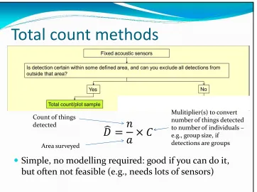
Total count methods

Simple, no modelling required: good if you can do it,

but often not feasible (e.g., needs lots of sensors)

Count of things detected

Area surveyed

Mulitiplier(s) to convert number of things detected to number of individuals – e.g., group size, if detections are groups

F ig . fr o m h tt p :/ /s e a g ra n t. m it .e d u /c fe r/ a c o u s ti c s /e xs u m /j a rv is /e x te n d e d .h tm l T h a n k s t o D . M o re tt i.

Image: Diane Claridge

Example: Dive counting for

beaked whales at AUTEC

Identify time and approximate location

of start of a group dive

Assume certain detectability

Assume can tell whether inside or out of survey area

area monitored

Example: Dive counting beaked

whales at AUTEC range

Issues:

sand rcome from different time and small samples

dive counting hard to automate groups diving close together

number of dive starts

mean group size from separate visual surveys

time spent monitoring

mean dive rate taken from a sample of tagged whales

̂

̂

Example: Sperm whales at AUTEC

Ward et al. (in press)

Sophisticated acoustic processing let us count all

sperm whales on the range in a sample of 50 10-minute

periods

Treat time periods as “snapshots”

To convert to density, needed to account for

availability: proportion of 10 minute periods an animal

will vocalize

Estimated using a separate dataset of tagged animals

(from same place but different time)

Distance

sampling

methods

25

Example: North pacific right whales

in the Bering sea

Marques et al. (2011) Example of cue count method

3 autonomous sensors over May-Oct, approx. 370 days of recordings

Data processed to obtain distances to right whale up calls

Example: North pacific right whales

in the Bering sea

Fitted detection function

Assuming a triangular distribution of animals about the

hydrophones,

̂

0.29

1.8%

1

̂

̂

area monitored

number of cues (up-calls) detected

Example: North pacific right whales

in the Bering sea

Cue count method (with allowance for mis-classification)

estimated proportion of false positives (from a manually processed sample)

estimated average detection probability of an up-call within the area monitored

time spent monitoring (summed over the ksensors)

estimated cue rate

Example: North pacific right whales

in the Bering sea

Issues:

Only 3 sensors, non-randomly placed, so assumption

that true distribution of call distances is triangular is

tenuous

With only 3 sensors, variance estimation is problematic

Call rates used may not be representative (obtained from

groups found because they were vocalizing?)

(For other issues, see Marques et al. 2011)

Example:

Fin whales in the Gulf

of Cadiz

Harris (In prep – PhD thesis)

Data from OBS: 24 points, each with 4 sensors –

can get distances.

Better example because

there are more points

!

Assumption of

1

̂

Example:

Fin whales (contd.)

Could treat as a cue count – methods would be just the

same as the right whale example

Alternatively, if you could track individuals within range

of each sensor, could use a snapshot approach

Assuming all individuals can be tracked at zero distance,

you get:

number of individuals detected

area monitored

estimated average detection probability of an individual at a snapshot moment (from standard detection function modelling)

number of snapshots

estimated proportion of false positives

Cue counting vs snapshots

Cue counting pros

Easy to identify cue

Occurs at an instant so no need to worry about movement

Cue counting cons

Need cue rate multiplier

Detection of cues may not be independent

Snapshot pros

No need for cue rate mulitplier

Snapshot cons

Need to be able to count individuals

What snapshot interval/spacing to use: arbitrary Need to be careful with variance estimation Ad hoc

Would be better to have methods that explicitly

Density without

distances: SECR

Spatially Explicit Capture Recapture

•

Borchers & Efford 2008

•

Borchers in press

An animal’s capture history

tells us something

(0,0,1,1,0,1,1,0,0)

But it can tell us more, it has a

spatial component usually

ignored

(0,0,8,12,0,11,7,0,0)

Example: Small mammal survey 16 traps, 9 capture sessions

SECR for acoustic data

You can treat a sound like an animal:

it starts from a single location (the

“home range center”) and radiates out,

being detected (“trapped”) at various

hydrophones (“traps”) (Efford et al. 2009; Dawson

and Efford 2009)

You only need one “trapping occasion” as the same

sound can be detected at multiple hydrophones

Example: Minke whales at PMRF

We used 16 hydrophones at the

Pacific Missile Range Facility

(PMRF), off Kauaii, Hawaii

Minke whale “boings” were detected, and TDOA and

dominant frequency were used to associate calls across

Image: Reefteach

Example: Minke whales at PMRF

Marques et al. (in press)

Proof of concept analysis: six 10-minute

sample periods were fit using secr package in

R (and a Bayesian approach)

Issues:

No accounting for islands (partially rectified in the follow-up paper)

Too few time periods (rectified in follow-up) So far, we just assumed that animals are uniformly distributed through the area

No cue rate available so only obtain density of cues (preliminary estimate used in follow-up)

Beyond SECR

SECR makes use of associations – can think of this as giving

information about locations but with measurement error

But in many cases you have more information about

location of sound:

Can often localize some sounds

Relative received levels may contain information about relative distances.

Ditto for frequency components

Sometimes you have bearing information

Density without

distances:

det. prob. from

auxiliary information

This is a worst-case scenario, as

you need to rely on auxiliary

information not part of the main

survey to get detection

probability

Just as with all multipliers, you

need to be careful this

information is applicable

39 See Borchers 2002

Example: Baltic harbour porpoises

with auxiliary visual observations

Kyhn (2010); Kyhn et al. (In press) Evaluation of concept: density estimation from T-PODs

T-PODs are porpoise detectors – record detection of porpoise clicks T-PODs were deployed at Fyns Hoved, Denmark close to shore, overlooked by visual observers Snapshot-based method: object counted is the number of 15s intervals where porpoises are detected (assumes max 1 porpoise) Detection probability obtained by using visual observers to set up trials

1

̂

Example: Baltic harbour porpoises

Getting the p:

Observers tracked porpoises visually. Assuming linear movement between surfacings, this gives us a patch. Can therefore estimate true position every 15 seconds.

Model the relationship between probability of detection against distance

Assuming triangular distribution of animals around hydrophone, can get average p

This approach is called a “trapping point transect” in the terrestrial

literature (Buckland et al. 2006) Example detection function _{(unpublished)}

Example: Baltic harbour porpoises

Issues:

Assumes max 1 animal per snapshot

Assumes triangular distribution of

animals around the T-POD

Example: beaked whales at AUTEC

with auxiliary tag data

Marques et al. (2009)

Cue-based method –

object counted is beaked

whale clicks over 82

hydrophones for 6 days

Detectability estimated

from separate tagging

experiment to set up trials

Detection function

estimated by logistic

regression – more complex

than porpoise as covariates

were used

Example: beaked whales at AUTEC

Issues:

Tag data was not collected at the same time as the main dataset. For one thing, the weather was calmer, on average when tags deployed. See Ward et al. (2011) for more on this.

Note:

False positive rate in this case study was around 50%! Doesn’t matter what it is, so long as you can characterize it precisely.

Example: Beaked whales via

acoustic modelling

Kusel et al. (2011); see also Harris (In prep PhD thesis) for a

blue whale example

Here, we use assumptions about source level combined

with acoustic modelling of transmission loss and detector

characterization to predict the detection function, and

then estimate

p

.

Source level distribution

Acoustic propagation

model

Detector performance Ambient

noise distribution Animal

location

distribution average prob of detection,

p

Example: Beaked whales via

acoustic modelling

Used 6 days of click detection data from 1 hydrophone

Cue counting estimator, just like Marques et al. (2009)

except

p

obtained from modelling rather than tag data

1

̂

Example: Beaked whales via

acoustic modelling

47

Estimating p:

Animal distribution and orientation – assumed uniform in x,y, depth from literature

Source level and beam pattern – from literature

Propagation model – Bellhop

Ambient noise – measured at different hydrophones from the one used to estimate density (not ideal)

Detector characterization – measured from small sample of marked-up data (not ideal)

All of these integrated in a Monte-Carlo simulation to estimate average p

Comments on acoustic modelling

approach

Advantage (relative to other auxiliary information

methods): no expensive tagging/visual observations

needed

Disadvantage: answers only as good as the modelling!

Summary – methods considered

Towed acoustic line transects on individuals/groups

Fixed sensors:

Plot sampling on cues (Beaked whale dive starts) and

individuals (sperm whales)

Point transects on cues (right whales) and individuals

via snapshot (fin whales)

SECR on cues (minke whales)

Trapping point transect on individuals via snapshot

(harbour porpoise) and cues (beaked whales)

Cue counting with

p

estimated from acoustic modelling

(beaked whales and blue whales)

Methods for

fixed

Conclusions

Estimation of whale density from passive acoustics

is a rapidly developing and expanding field

Which method when? – hopefully roadmap will

help

Density estimation often hampered by lack of

auxiliary data, e.g., vocalization rates

Need more studies on basic acoustic ecology

Conclusions

Survey design is a critical issue

Good spatial and temporal coverage of samplers

Minimize use of multipliers (e.g., use individuals rather

than cues; certain detection rather than

p

)

Measure multipliers as part of the main survey (e.g., get

distances to estimate

p

). If not possible, use a good

sampling design in same time and place as survey. If not

possible, do this with any component you can (e.g.,

detector characterization)

Need for development of inexpensive, capable and

accessible hardware

References

Barlow, J. & Taylor, B. 2005. Estimates of sperm whale abundance in the northeastern temperate Pacific from a combined acoustic and visual survey Marine Mammal Science 21, 429-445

Borchers, D.L., S.T. Buckland and W. Zucchini. 2002. Estimating Animal Abundance: Closed Populaitons. Springer. Borchers, D.L. In press. A non-technial overview of spatially explicit capture recapture models. Journal of Ornithology. Borchers, D. & Efford, M.2008. Spatially explicit maximum likelihood methods for capture-recapture studies Biometrics, 64, 377-385

Buckland, S.T., R.W. Summers, D.L. Borchers and L. Thomas. 2006. Point transect sampling with traps or lures. Journal of Applied Ecology 43: 377-384. Dawson, D. K. & Efford, M. G. 2009. Bird population density estimated from acoustic signals. Journal of Applied Ecology. 46, 1201-1209 DiTraglia, F.J. 2007. Models of Random Wildlife Movement with an Application to Distance Sampling. MMaths Statistics, University of St Andrews Efford MG, Dawson DK, Borchers DL 2009 Population density estimated from locations of individuals on a passive detector array. Ecology 90:2676-2682

Hastie, Swift, Gordon, Slesser and Turrell. 2003. Sperm whale distribution and seasonal density in the Faroe Shetland Channel. Journal of Cetacean Research Management 5: 247-252.

Kyhn, L.A. 2010: Passive acoustic monitoring of toothed whales, with implications for mitigation, management and biology. PhD thesis. Dep. of Arctic Environment, NERI, Aarhus University. National Environmental Research Institute, Aarhus University, Denmark

Kyhn L.A., J. Tougaard, L. Thomas, L.R. Duve, J. Steinback, M. Amundin, G. Desportes and J. Teilmann. In Pres. From echolocation clicks to animal density - acoustic sampling of harbour porpoises with static dataloggers. Journal of the Acoustical Society of America.

Küsel, E.T., D.K. Mellinger, L. Thomas, T.A. Marques, D.J. Moretti, and J. Ward. 2011. Cetacean population density from single fixed sensors using passive acoustics. Journal of the Acoustical Society of America 129: 3610-3622.

Lewis, Gillespie, Lacey, Matthews, Danbolt, Leaper, McLanaghan, Moscrop. 2007. Sperm whale abundance estimates from acoustic surveys of the Ionian Sea and Straits of Sicily in 2003. J Mar Biol Assoc UK 87: 353-357.

Marques, T.A., L. Thomas, J. Ward, N. DiMarzio, P. L. Tyack. 2009. Estimating cetacean population density using fixed passive acoustic sensors: an example with beaked whales. Journal of the Acoustical Society of America 125: 1982-1994.

Marques, T.A., L. Thomas, L. Munger, S. Wiggins and J.A. Hildebrand. 2011. Estimating North Pacific right whale (Eubalaena japonica) density using passive acoustic cue counting. Endangered Species Research 13: 163-172

Marques, T. A., Thomas, L., Martin, S. W., Mellinger, D. K., Jarvis, S., Morrissey, R. P., Ciminello, C., DiMarzio, N. In press. Spatially explicit capture recapture methods to estimate minke whale abundance from data collected at bottom mounted hydrophones. Journal of Ornithology.

Martin, S.W., T.A. Marques, L. Thomas, R.P. Morrissey, S. Jarvis, N. DiMarzio, D. Moretti and D. Mellinger. In press. Estimating minke whale (Balenoptera acutorostrata) boing sound density using passive acoustic sensors. Marine Mammal Science.

Mellinger, D.K., S.W. Martin, R.P. Morrissey, L. Thomas and J.J. Yosco. 2011. A method for detecting whistles, moans and other frequency contour sounds. Journal of the Acoustical Society of America 129: 4055-4061

Moretti, D., T.A. Marques, L. Thomas, N. DiMarzio, A. Dilley, R. Morrissey, E. McCarthy, J. Ward and S. Jarvis. 2010. A dive counting density estimation method for Blainville's beaked whale (Mesoplodon densirostris) using a bottom-mounted hydrophone field as applied to a Mid-Frequency Active (MFA) sonar operation. Applied Acoustics 71: 1036-1042.

Rankin, S, and J. Barlow. 2005. Source of the North Pacific ‘boing’ sound attributed to minke whales. Journal of the Acoustical Society of America 118(5):3346-51. Ward, J.A., L. Thomas, S. Jarvis, N. DiMarzio, D. Moretti, T.A. Marques, C. Dunn, D. Claridge, E. Hartvig and P. Tyack. Submitted. Passive acoustic density estimation of sperm whales in the Tongue of the Ocean, Bahamas.

Ward, J., Jarvis, S., Moretti, D., Morrissey, R., DiMarzio, N., Thomas, L. and Marques, T. 2011. Beaked whale (Mesoplodon densirostris) passive acoustic detection with increasing ambient noise. Journal of the Acustical Society of America 129: 662-669.

Dealing with g(0)<1:

perception bias

Steve Buckland

Centre for Research into Ecological

and Environmental Modelling,

University of St Andrews

Dealing with g(0)<1:

perception bias

Steve Buckland

and David Borchers

Centre for Research into Ecological

and Environmental Modelling,

P ro b a b il it y o f d e te ct io n g ( x ) 1.0

Distance from line x

Conventional distance sampling (cds)

g(0) = 1

The detection function g(x)

Probability of detection as a function of distance from the line

P ro b a b il it y o f d e te ct io n g ( x ) 1.0

Distance from line x

The detection function g(x)

Probability of detection as a function of distance from the line

Perception bias – some animals that are on the line and available to be seen are missed.

cds biased by -25%

P ro b a b il it y o f d e te ct io n g ( x ) 1.0

Distance from line x

The detection function g(x)

Probability of detection as a function of distance from the line

Mark-recapture distance sampling (mrds)

g(0) < 1

P ro b a b il it y o f d e te ct io n g ( x ) 0.8

Distance from line x

The detection function g(x)

Probability of detection as a function of distance from the line

0.6

Availability bias – animals that were on the line but

unavailable to be seen

mrds biased by -20%

Are ‘independent observers’ really independent?

Suppose we have 2 observers, A and B, and 200 whales.

Suppose for each observer, 100 whales have probability

of detection p = 0.75 and 100 have p = 0.25.

(We ignore for now the effect of distance from the line on

probability of detection.)

If the observers are independent, then the probability that B

detects a whale is unaffected by whether A detects that whale.

Are ‘independent observers’ really independent?

100 whales have p = 0.75 and 100 have p = 0.25.

B expects to detect 75 + 25 whales, so if we cannot identify

whether a whale belongs to the first or second group, its

(unconditional) prob of detection by B is 100/200 = 0.5.

Example: pack-ice seals

Observer 1 detections

Proportion

of Observer 2 detections seen by Observer 1

Unmodelled Heterogeneity

here

Are ‘independent observers’ really independent?

Conclusion:

Even if two observers operate entirely independently, we

cannot assume that whether one observer detects a whale is

independent of whether the other observer detects it.

However, if for each whale detected, we were able to identify

Are ‘independent observers’ really independent?

Generalizing, if we can record covariates that fully explain

the variability in detectability among whales, and incorporate

those covariates in our detection function, we can assume

that the observers are independent and we can use a full

independence model.

In reality, we will be unable to record all relevant covariates,

and our detection function model will be imperfect. In this

circumstance, including covariates in our model will reduce

the dependence between observers, but not eliminate it.

How does distance from the line affect the

independence assumption?

Far from the line, many animals have very low probability

of detection, while a few (e.g. those in large groups, active at

the surface, in sea state 0) may be easily detected.

Close to the line, the heterogeneity in the detection probabilities

will tend to be much smaller (e.g. seals in pack-ice), and hence the

conditional probability that one observer detects a whale given that

the other does will be much closer to the unconditional probability.

Point independence exploits this by assuming that independence

How does distance from the line affect the

independence assumption?

In reality, some degree of dependence is still likely to occur

even on the line, especially when mean probability of detection

on the line is appreciably less than one.

If we consider the limit as probability of detection tends to one,

then independence must apply, as there will no longer be any

heterogeneity in the detection probabilities.

This is the idea underlying limiting independence.

Model selection

•

Point independence and full independence

models are special cases of a general

limiting independence model

•

So we can use e.g. AIC to decide whether a

point independence or a full independence

model is adequate given our data

Estimation

For single-observer line transect surveys, there is no information

in the data to allow estimation of g(0), the probability of

detection of an animal that is on the line.

Visual Mark-Recapture

Obs 2

=“trapping occasion”

Seen by 2

=“marked”

Obs 1

=“trapping occasion”

Visual Mark-Recapture

Obs 2

=“trapping occasion”

Obs 1

=“trapping occasion”

Passes unseen by 1

Seen by 2

=“marked”

Seen by 2

=“marked”

Seen by 1

Estimation

By adding a mark-recapture component to the likelihood,

we lose the ‘pooling robust’ property of line transect

estimators, and so it becomes important to model

heterogeneity through covariates.

What sources of heterogeneity should be measured?

Sources of Heterogeneity

• The animals themselves (distance, size, behavior, ...)

• The environment (sea state, visibility, ...)

Group size

• The kind of survey effort (the observers, their platforms, ...)

Observer

Configuration:

Trial-Observer

Observer 2

Observer 1

sets up trials for

to estimate

p

The Observer at the end of an arrow must be

independent of

Configuration:

Independent Observer

Observer 2

Observer 1

sets up trials for

to estimate

p

to estimate

p

The Observer at the end of an arrow must be

independent of

the Observer at the start of the arrow

p

= p

+

p

-

(

p

p

)

Abundance Estimation

• Trial-Observer

• Independent Observer

∑

=

1

ˆ

(

,

)

Field methods

• Use a dedicated “duplicate identifier”

• Record measure of confidence in duplicate identification.

• Record positions and times as precisely as possible

• Record ancillary data

• Have at least one observer “track” animals

Duplicate Identification

Analysis methods

• Bracket "best" estimate by two extremes

• Rule-based duplicate identification after the survey. (e.g.

Schweder et al., 1996)

• Probabilitistic duplicate identification after the survey.

(e.g. Hiby & Lovell, 1998)

Schweder, T., Hagen, G., Helgeland, J. and Koppervik, I. 1996. Abundance estimation of northeastern Atlantic minke whales. Rep. Int. Whal. Commn. 46: 391-405. Hiby, A. and Lovell, P.1998. Using aircraft in tandem formation to estimate abundance of

harbour porpoise. Biometrics 54: 1280-1289.

Estimation with incomplete detection

at distance zero

“g(0)<1”

Laake, J.L. and Borchers, D.L. 2004. Methods for incomplete detection at distance zero. Chapter 6 in Advanced Distance Sampling (eds S.T. Buckland, D.R. Anderson, K.P. Burnham, J.L. Laake, D.L. Borchers, L. Thomas). OUP. Borchers, D.L., Laake, J.L., Southwell, C. and Paxton, C. 2006.

Accommodating unmodeled heterogeneity in double-observer distance sampling surveys. Biometrics 62: 372-378

Buckland, S.T., Laake, J.L. and Borchers, D.L. 2009. Double-observer line transect methods: levels of independence. Biometrics 66: 169-177 Laake, J.L., Collier, B.A., Morrison, M.L. and Wilkins, R.N. 2011.

Dealing with g(0)<1

Availability bias

Hans J. Skaug

Department of mathematics University of Bergen

Norway

Availabilty bias: diving whales

• Whales can only be detected at surface

D

e

p

th

2

0

0

1

0

0

Long versus short diving whales

D

e

p

th

0 100 200 300 400 seconds

0 100 200 300 400 minutes

Minke whale dive pattern

• Multiple cues made within detectable range of observer (< 1000m) • Topic of this lecture

Sperm whale dive pattern.

•Long (deep) dives during which the observer can pass the whale •See Okamura et al. (2011)

Availability bias caused by diving

• Whales on the trackline may be diving when passed by the observer

g(0) < 1

• Diving pattern in front of observer determines the probablity of detection – Diving pattern = heterogenity factor – At ”animal” level

• Diving pattern only partly observed – ”Diving pattern” is not simple covariate – Difficult to account for in standard

statistical analysis

Minke whale diving behaviour

Sighting surveys: # cues per animal in front of observer

Number of cues

F re q u e n c y

0 5 10 15

0 1 0 0 2 0 0 3 0 0 4 0 0

0 2000 4000 6000 8000 10000 12000

Surfacing times from a radio tagged whale

Seconds

Internal data

Number of times the observer saw the whale at surface • Selection bias

External data

Time points when the whale was at surface from radio-tagging a minke whale • Small number of animals

Poisson process model

• Assumption: dive times

follow Poisson process with intensity αsurfacings/second

1. Individual dives exponentially distributed

2. Dive times are serially independent (no correlation)

• Not a perfect dive time model for minke whales

Minke whale dive times from radio tags

Duration of dive (seconds)

D e n s it y

0 50 100 150 200

0 .0 0 0 0 .0 0 5 0 .0 1 0 0 .0 1 5 Exponential distribution

Serial correlation in minke whale dive times (radio tags):

Hazard models for the

detection function

• If you accept that dive times follow a Poisson

process you have to (mathematically) accept the

hazard model for the detection function

0

Perpendicular distance

( )

Pr(detect animal at distance x)

g(x)

1 exp

( , )

x

g x

h x y dy

v

α

=

=





= −



−





∫



Surfacing rate

Observer speed

Forward distance

Hazard probability function

Hazard probability: h(x,y)

• Probability of detecting individual

cue/surfacing = h(x,y)

• Multiple opportunities for detecting

the whale

– g(x) is the ”total probability” of

detecting the whale

Independent observers

and discrete availablity

• Two independent observers: A and B

• Positive ”dependene” between A and B

g

(x) > g

(x) g

(x)

– B-detects

→

_{increased probability of}

A-detects.

• What does «independent observer» mean?

– Independence at cue/surfacing level

h

(x,y) = h

(x,y) h

(x,y)

Not full independence: gAB(x) ≠ gA(x) gB(x)

Full independence versus discrete availablity

0 500 1000 1500

0 .0 0 .2 0 .4 0 .6 0 .8 1 .0 g (y ) Only A A and B; full independence A and B; discrete availablity Bias due to erroneously assuming full independence If you also take into account estimation of h(x,y) the bias in ESHW is 30%

(Skaug&Schweder, 1999) A alone

Ending remarks, future

development

• Not integrated into standard software

packages (Distance)

– Limits the use of the approach

• To which extent can point independence

account for discrete availablity?

• Robustness of the hazard probability

model wrt. choice of parametric form of

h(x,y) has been studied (Kleppe et al,

2010)

References

• Buckland, S. T., Anderson, D. R., Burnham, K. P., Laake, J. L., Borchers, D. L., and Thomas, L. (2004). Advanced Distance Sampling ({Oxford: Oxford University Press}).

• Okamura, H., Kitakado, T., Hiramatsu, K., and Mori, M. (2003). "Abundance Estimation of Diving Animals by the Double-Platform Line Transect

Method," Biometrics 59, 512-520.

• Kleppe, T., Skaug, HJ., Okamura, H. (2010) Asymptotic bias of the hazard probability model under model mis-specification. J. Cetacean Res. Manage. 11(3): 249-252, 2010

• Schweder, T., Skaug, H. J., Langaas, M., and Dimakos, X. (1999). "Simulated likelihood methods for complex double-platform line transect surveys," Biometrics 55, 678-687.

• Skaug, H. J., and Schweder, T. (1999). "Hazard models for line transect surveys with independent observers," Biometrics 55, 29--36.

Tore Schweder

New Developments in Cetacean Survey Methods

Dealing with Measurement Error

David Borchers & Tiago Marques

Measurement Errors

y

r

θ

o

r

θ

X _X

1. Rounding to favored values Biased Estimates

–

(Also called “heaping”)

–

Rounding to zero most serious

–

Can be dealt with by grouping

–

(Smearing: ad-hoc; introduces dependence)

2. Biased measurement Biased Estimates

–

Regression correction method: correct distances before

fitting; neglects variance

3. Random measurement errors Biased Estimates

–

Worse for point transects than line transects

–

Negatively Biased variance and CI estimates

The Problem

1. Regression bias correction methods (various authors) 2. Smearing (developed for rounding errors)

– Butterworth (1982): ad-hoc method; Buckland & Anganuzzi (1988) improved 3. Hiby et al. (1989): MLE for cue-counting with grouped distance data,

allowing g(0)<1

4. Alpizar-Jara (1997), Chen (1998), Chen & Cowling (2001)1_{: Line Transect}

with additive distance errors

5. Marques (2004): Line Transect with multiplicative distance errors

6. Borchers et al. (2009, 2010a) Line & Point Transect with any kind of errors

7. Schweder et al (1999) Method of simulated likelihood for errors with instantaneous hazard & Poisson availability

r

Data on Measurement Error

x

(Borchers et al 2010)

r

(Borchers et al 2010)

1: Method of Leaper et al. 2010

Regression Bias Correction Method(s)

Estimated=True

Regression:

Estimated=B×True

Estimated Bias

X

=

X

÷

B

X

X

Estimate using

X

Correction Factor Methods

• Line Transects

– Density estimator:

– Multiplicative error:

x

x

ε

• Variance & CI

– Bootstrap for correction factor – Delta method

ˆ

D

=

n

×

ˆf(x

=

0)

2WL

ˆ

D

=

n

×

ˆf(x

=

0)

2WL

÷

ˆ

E

1

ε









Fitted to observed distances (with measurement error)

Estimated from pairs of

trueand measureddistances

Correction Factor Methods

• Point Transects

– Density estimator:

– Multiplicative error:

r

r

ε

• Variance & CI:

ˆ

D

=

n

×

h(r

ˆ

=

0)

π

K

ˆ

D

=

n

×

h(r

ˆ

=

0)

π

K

÷

ˆ

E

1

ε









Fitted to observed distances (with measurement error)

Estimated from pairs of

Potential problem with Correction Factor Methods

May choose wrong model by fitting to observed distances (those with measurement error)

More General (but less convenient) Method

• Conventional Distance Sampling (CDS) likelihood:

• Likelihood with Measurement Error:

• Likelihood with Measurement Error and Experiment Data:

• Variance & CI: bootstrap

L(

φ

)

=

f (x

;

φ

)

i=1

n

∏

L(

φ

|

β

)

=

f (x;

φ

)

×

δ

(x

| x;

β

)dx

0

∞

∫

i=1

n

∏

Measured distance

Unobserved True distance

Measurement Error Model

L(

φ

,

β

)

=

L(

φ

|

β

)

×

f (x

| x

;

β

)

j=1

m

∏

Estimator %Bias (small sample: LT n=60; PT n=80)

½norm narrow

½norm wide

hazard rate

Variance and CI Coverage

• Correction factor CI:

– (Marques, 2004, Table 1) – Blue=CDS; Red=Corrected

• MLE CVs

– Cue-counting survey:

• Point estimate: MLE 9% lower than CDS • MLE CI width: 58% wider than CDS – Line Transect survey:

• Point estimate: MLE 9% lower than CDS • MLE CI width: MLE 19% wider than CDS

What about when g(0)<1?

• Have duplicates, so don’t have to have experimental (true,

estimated) data (although it helps): duplicates allow

estimation of error process (with assumption of common process)

• Hiby et al. (1989): cue-counting with grouped distances

• Schweder et al. (1999): Method of Simulated Likelihood. Uses 2-D detection hazard and Poisson availability

Preliminary Results using SECR MLE Method

(If available in time, some Line Transect Simulation Results to go here)

Preliminary Results using SECR MLE Method

Summary

• Systematic errors (measurement bias) always a problem. • Random errors add variance but little bias with CDS1_if

– Error CV < about 30% for Line Transects

– Error CV < about 10% for Point Transects (& Cue-counting)

• Correction factor method easy (can use Distance) but occasionally does not work well (esp. Point Transects)

– Only applies with multiplicative error models

• Full likelihood method works well (but no general user-friendly software available)

– Applies with any error model • SECR Method under development

• Should incorporate uncertainty associated with measurement error.

Alpizar-Jara, R. 1997. Assessing assumption violation in line transect sampling. PhD thesis, North Carolina State University, Raleigh.

Borchers, D.L., Pike, D. Gunlaugsson, Th. and Vikingsson, G.A. 2009. Minke whale abundance estimation from NASS 1987 and 2001 cue-counting surveys taking account of distance estimation errors. North Atlantic Marine Mammal

Commission Special Issue 7: 95-110.

Borchers, D.L., Marques, T.A., Gunnlaugsson, Th. and Jupp, P. 2010a. Estimating distance sampling detection functions when distances are measured with errors. JABES DOI: 10.1007/s13253-010-0021-y.

Borchers, D.L. 2010b. A non-technical overview of spatially explicit capture–recapture models. Journal of Ornithology. DOI: 10.1007/s10336-010-0583-z

Buckland, S.T. and Anganuzzi, A. 1988. Comparison of smearing methods in the analysis of minke sightings data from IWC/IDCR Antarctic cruises. Report of the International Whaling Commission 38: 257-263.

Butterworth, D.S. 1982. On the functional form used for g(y) form minke whale sightings, and bias in its estimation due to measurement inaccuracies. Report of the International Whaling Commission 32: 833-838.

Chen, S.X. 1998. Measurement errors in line transect surveys. Biometrics 54: 899-908.

Chen, S.X. and Cowling, A. 2001. Measurement errors in line transect sampling where detectability varies with distance and size. Biometrics 57: 732-742.

Hiby, L., Ward, A. and Lovell, P. 1989. Analysis of the North Atlantic sightings survey 1987: Aerial survey results. Report of the International Whaling Commission 39:447-455.

Leaper, R., L. Burt, and D. Gillespie, and K. MacLeod. 2010. Comparisons of measured and estimated distances and angles from sighting surveys. Journal of Cetacean Research and Management 11:229-37.

Marques, T.A. 2004. Predicting and correcting bias caused by measurement error in line transect sampling using multiplicative error models. Biometrics 60: 757-763.

Royle, J.A. and Dorazio, R.M. 2008. Hierarchical modelling and inference in ecology. Academic Press. London. Schweder, T., Skaug, H.J., Langaas, M. and Dimakos, X.K. 1999. Simulated likelihood methods for complex

double-platform line transect surveys. Biometrics 55: 678-687.

Williams, R., Leaper, R. Zerbini, A.N. and Hammond, P.S. 2007. Methods for investigating measurement error in cetacean line transect sur eys. Journal of the Marine Biological Association of the UK 87: 313-320.

Habitat-based Models of Cetacean Density

in the eastern Pacific

WHY IS CETACEAN DENSITY

IMPORTANT?

•

Plan potentially harmful human activities to

avoid areas of high cetacean density

•

Estimate the number of animals potentially

affected by human activities

Density = # animals per km

2

SURVEY EFFORT AND BLUE

WHALE SIGHTINGS: 2001

Why model density?

Data are sufficient only to

estimate density w/in the

entire study area

OBJECTIVES

Develop methods to model and predict

cetacean density based on environmental

variables.

TECHNICAL APPROACH

Cetacean Survey Data

Habitat Data

Mathematical Models of Cetacean Density

Cetacean Survey

Data 1986-2006:

•

Ship and aerial surveys

Southwest Fisheries

Science Center

Habitat Data

1986-2006:

•

Oceanographic data

from

Southwest

Cetacean

Line

‐

transect

Surveys

by

the

Southwest

Fisheries

Science

Center

3

Observers

two

25x

“big

eyes”

binoculars

one

7x

binocular

&

naked

eye

Reticles

(distance)

Striped Dolphins:

1986-2006 SWFSC Surveys

Density Modeling Methods

1. Divide your transects

into segments of

roughly uniform length.

2. Tally all the sightings

that occur on each

segment (n = #

sightings).

3. Estimate mean group

size for each segment

that contains a sighting.

4. Create a data frame

(spreadsheet) with

Segment

Length

#

sightings

group

size

1

10

0

2

10

2

10.2

3

11

0

4

11

1

8

5

10

0

Density Modeling Methods

1. Add location info for

each segment.

2. Add habitat variables for

each segment.

Length #

sightings group

size

Latitude Longitude

Depth

SeaSurf

Temp

Thermo

‐

cline

D

10

0

59.3

‐

125.2

120

12.2

50

10

2

10.2

59.0

‐

125.5

550

13.4

40

11

0

58.7

‐

125.7

600

15.3

30

11

1

8

58.4

‐

125.5

604

13.2

40

10

0

58.1

‐

125.1

400

10.2

30

HABITAT VARIABLES

•

NMFS/SWFSC Ecosystem Data from Cetacean Surveys:

1.) sea surface temperature

2.) sea surface salinity

3.) thermocline depth

4.) thermocline strength

5.) surface chlorophyll concentration

6.) Beaufort sea state

7.) latitude

8.) longitude

•

NOAA NGDC’s TerrainBase Global Terrain:

1.) water depth

Æslope

Line-transect Modeling Approach

using Generalized Additive Models

Encounter Rate (ER=n/L = # sightings / distance surveyed)

•

log(n) = mean + f(oceo) + f(geo) + log(L) + error

•

error ~ quasi-likelihood distribution

variance proportional to mean

log link w/ distance surveyed (L) as an offset

Group Size (s)

•

log(s) = mean + f(oceo) + f(geo) + error

Spatial Model Nomenclature

Habitat suitability model:

presence/absence info

habitat data

Spatial density model:

line-transect survey info

spatial coordinate data

Habitat-based density model:

line-transect survey info.

habitat data

Marine Mammal Density Modeling

Sighting Data

Effort Data

Habitat Data

Preliminary Density Models

Best & Final Density

“Acceptable” Density

Models

Review

Team

ADVANCING THE SCIENCE OF

PREDICTIVE DENSITY MODELING

MODELING FRAMEWORK

Generalized Linear Models

Generalized Additive Models

Tree-based models

Area effectively search as offset

ERROR STRUCTURE

Poisson

Quasi-likelihood

Negative Binomial

DATA SOURCES

In situ

EFFECT OF SPATIAL

RESOLUTION

Blue whale prediction ratios (observed/predicted)

10 km

20 km

40 km

80 km 160km

1986

0.714

0.700

0.788

0.654

0.627

1988

1.383

1.419

1.246

1.144

1.179

1989

1.618

1.598

1.339

1.367

1.356

1990

1.937

1.989

1.926

2.143

1.877

1998

0.628

0.707

0.651

0.720

0.586

1999

0.583

0.627

0.627

0.709

0.626

2000

1.075

1.174

1.030

0.945

1.163

EFFECT OF SPATIAL EXTENT

California

Current

Ecosystem

EFFECT OF SPATIAL EXTENT

Eastern Tropical Pacific

California Current Ecosystem

Eastern Tropical Pacific & California Current, combined

Ecosystems

are best

Model Comparisons

for striped dolphins:

Remotely Sensed vs.

In Situ Data

(left vs. right)

Generalized additive vs.

Generalized linear models

(top vs. bottom)

Mid-Trophic Data Sources

Oceanographic Data

Oceanographic Data + Acoustic

Backscatter & Net Tow Data

Does the inclusion of

data from mid-trophic

components of the

food web improve our

models of cetacean

density?

Mid-trophic data

Short-beaked

Common

Dolphin

Density per Square

Kilometer

Preview of preliminary cetacean density

models for the Central Pacific

California

Current

Eastern

Tropical

Pacific

Central Pacific

Co-PIs

Elizabeth Becker

Karin Forney

Jay Barlow

(SWFSC)

Dave Foley

CenPac: Include area effectively searched as an offset

“Encounter rate” (

n

/

A

):

ln(

n

) = offset(

A

) + f(SST) + ....

Group Size (

s

):

ln(

s

) = f(SST) + f(depth) + ....

**ESW calculated per segment using multi-covariate approach

(Barlow et al. NOAA Tech Memo)

D = (

n

/

A

)*

s

*g(0)

-1

A = 2*L*ESW

Poor viewing

conditions

Fair viewing

conditions

Great viewing

conditions

Estimation of segment-specific

effective area searched, A

_E

= 2*L*ESW

Key effects on viewing conditions:

•

Beaufort sea state (0-6)

•

Swell height (deviation from Beaufort expectation)

•

Visibility (in nmi)

Integrating new satellite-derived products into

habitat-based density models

Global High Resolution SST

(GHRSST)

Multi-sensor approach (“blended SST”)

z

High-resolution infrared data

z

Microwave (data for cloudy areas)

z

Optimal interpolation

z

Pixel-by-pixel error characterization

Developed by Remote Sensing

Co-PIs

Elizabeth Becker

Karin Forney

Jay Barlow

Jessica Redfern

(SWFSC)

Dave Foley

(JIMAR/SWFSC)

NOWCASTS

Estimate whale

density using habitat

models

Spatially Explicit Risk Assessment:

Large Whale Ship Strikes (Jessica Redfern)

Alternative shipping

routes derived from

shipping data

Habitat Models

• Fin and humpback whales have

opposing hot spots

• Blue whales are more evenly

Fin Whales

Blue Whales

Percent change in risk between the Channel and the alternate routes

Increase risk in

alternate routes

•

Strategic Environmental Research and Development

Program

•

NOAA Southwest Fisheries Science Center (mammal

observers, cruise leaders, survey coordinators,

oceanographers, plankton sorters, officers, crews)

•

Navy N-45 (Frank Stone & Ernie Young)

•

Steve Reilly, Robert Brownell & Lisa Ballance; Megan

Ferguson, Jim Carretta, Dave Foley & Ray Smith