A Retrospective Filter Trust Region Algorithm for
Unconstrained Optimization*
Yue Lu, Zhongwen Chen
School of Mathematics Science, Suzhou University, Suzhou, China E-mail: [email protected], [email protected]
Received June 8, 2010; revised July 18, 2010; accepted July 21, 2010
Abstract
In this paper, we propose a retrospective filter trust region algorithm for unconstrained optimization, which is based on the framework of the retrospective trust region method and associated with the technique of the multi-dimensional filter. The new algorithm gives a good estimation of trust region radius, relaxes the condi-tion of accepting a trial step for the usual trust region methods. Under reasonable assumpcondi-tions, we analyze the global convergence of the new method and report the preliminary results of numerical tests. We compare the results with those of the basic trust region algorithm, the filter trust region algorithm and the retrospective trust region algorithm, which shows the effectiveness of the new algorithm.
Keywords:Unconstrained Optimization, Retrospective, Trust Region Method, Multi-Dimensional Filter Technique
1. Introduction
Consider the following unconstrained optimization pro- blem
min f x (1) where x R n, :f Rn R is a twice continuously diff-
erentiable function.
The trust region method for unconstrained optimiza-tion is first presented by Powell [1], which, in some sense, is equivalent to the Levenberg-Marquardt method which is used to solve the least square problems and which was given by Levenberg [2] and Marquardt [3]. The basic idea of trust region methods works as follows. In the neighborhood of the current iterate (which is called the trust region), we define a model function that approximates the objective function in the trust region and compute a trial step within the trust region for which we obtain a sufficient model decrease. Then we compare the achieved reduction in f(x) to the predicted reduction in the model for the trial step. If the ratio of achieved versus predicted reduction is sufficiently positive, we define our next guess to be the trial point. If this ratio is not sufficiently positive, we decrease the trust region radius in order to make the trust region smaller. Other-wise, we may increase it or possibly keep it unchanged.
Since the trust region method is of the naturalness, the strong convergence and robustness, it has been con-cerned by many people, such as Powell [1,4,5], Schultz et al. [6], Sorensen [7], Moŕe [8], Yuan [9] and so on. In recent years, the trust region method has been applied to the optimization problems with equality constraints [10], simple bound constraints [11], convex constraints [12] and so on. Many of convergence results have been ob-tained, which can be seen in [13].
Fletcher, Leyffer and Toint [20] review the ideas above and mention the application of the filter method in prac-tice. In [14], they study the problem of the following form
min f x ,
. . 0
s t c x ,
where c R: nRm is continuously differentiable
func-tion. Define the measure of the constraint violation
1
max 0, .
m
j j
h c x c x
We use
f( )k ,h( )k
to denote values of f x
and
h c x evaluated at xk. Now, we give the following
definitions about the filter methods.
Definition 1.1 A pair
f( )k ,h( )k
obtained on iterationk is said to dominate another pair
f( )l,h( )l
if andonly if
( )k ( )l and ( )k ( )l .
f f h h
Definition 1.2 A filter is a list of pairs
f( )l ,h( )l
such that no pair dominates any other.
We use Fk to denote the set of iteration indices
j j k such that
f( )j,h( )j
is an entry in thecur-rent filter.
Definition 1.3 A pair
f( )l,h( )l
is said to be acce-ptable for inclusion in the filter if it is not dominated by any pair in the filter, that is, for any pair
f( )l,h( )l
k
F ,
f( )k ,h( )k
satisfies( )k ( )l or ( )k ( )l
f f h h (2) In order to obtain the global convergence of the algo-rithm, we should make f, h satisfy the sufficient reduc-tion condireduc-tion, so we strengthen the acceptable rule (2) as
( )k ( )l ( )l or ( )k 1 ( )l
h h
f f h h h (3) where h (0,1). When h (0,1) is very small, there
is negligible difference in practice between (2) and (3). Definition 1.4 When the pair
f( )k ,h( )k
is added tothe list of pairs in the filter, any pairs in the filter that are dominated by the new pair are removed, that is, we re-move the pair
( )l, ( )l
k
f h F which satisfies
( )k ( )l and ( )k ( )l .
f f h h
This is called the modification of the filter.
Gould et al. [21] and Miao et al. [22] applies the filter technique to unconstrained optimization, whose charac-teristic is to relax the condition of accepting a trial step for the usual trust region method, which improves the effectiveness of the algorithm in some sense. The non-monotonic algorithm also has the algorithm in some
sense. The nonmonotonic algorithm also has the charac-teristic [23,24].
Recently, Bastin et al. [25] presents a retrospective trust region method for unconstrained optimization. Comparing their algorithm with the basic trust region algorithm, the updating way of the trust region radius is different, and the retrospective ratio
1 1
1
1 1 1 1
1 1
k k k
k
k k k k k
k k k
k k k k k
f x f x s
m x m x s
f x f x s
m x m x s
is mentioned, where m xk
ks
is the approximated quadratic model of the objective function f x
at xk.k
s is a solution of the following trust region subproblem
min , . . .
k k k
m x s
s t s
(4)
k
is the trust region radius at the current iterate point. In the basic trust region algorithm, the ratio k
k
k k
k
k k k k k
f x f x s
m x m x s
plays the following two roles.
1) Determine the trial step to be accepted by the algo-rithm or not.
2) Adjust the trust region radius correspondingly. In the retrospective trust region method, the two roles are played by the ratio and , respectively. In the basic trust region algorithm, the determination of trust region radius is an important and difficult problem. Sart- enaer [26] and Zhang et al. [27] present the self-adaptive trust region methods and give some discussions about the determination of trust region radius. Bastin et al. [25] presents a retrospective trust region method for uncon-strained optimization. The retrospective ratio in this method uses the information at the current iterate and the last iterate point, which can give the more effective esti-mation of trust region radius. Hence, the number of solving trust region subproblem may be decreased, which improves the effectiveness of the method.
new algorithm. This paper is organized as follows. The new algorithm is described in Section 2. Basic assump-tions and some lemmas are given in Section 3. The analysis of the first order and second order convergence is given in Section 4 and Section 5, respectively. Section 6 reports the numerical results. Finally, we give some final remarks on this approach.
2. Algorithm
In this paper, we define ( )g x xf x( ). At the current iterate x fk, ( ), ( ), k f xk gk g xk gki denotes the ith
component of the vector gk. Throughout this paper,
denotes the Euclidean norm. Now, we review the basic-trust region algorithm as follows.
2.1. Algorithm BTR (Basic Trust Region Algorithm)
Step 0. (Initialization) Given an initial pointx0Rnand
an initial trust-region radius 0 0.0 1 21 and
1 2
0 1. Set k: 0 .
Step 1. (Model definition) Define a model function
k
m in k, where k
x R n| .x x k k
Step 2. (Step calculation) Compute a trial step sk for solving trust region subproblem (4).
Step 3. (Updating iterate point) Compute (f xksk) and the ratio
k
k k
.k
k k k k k
f x f x s
m x m x s
then,
1 1
1
, if , , if .
k k k
k
k k
x s x
x
Step 4. (Updating trust-region radius) Set
2
1 2 1 2
1 2 1
, , if , , , if , , , , if .
k k
k k k k
k k k
Set k: k 1, and go to Step 1.
In the algorithm BTR, we do not give a formal stop-ping criterion. In practice, the stopstop-ping criterion can be installed in Step 1, such as
max
or ,
k
g eps kk
where eps denotes the precision, and kmax denotes the
maximal number of iterations.
If x is a local minimizer of the problem (1), then
0g x . Motivated by the filter method, we set
g x to be the measure of the iterate. Now we
intro-duce some definitions about the multi-dimensional filter. Definition 2.1 We say that a point xk dominates
an-other point xl, if
for all 1, 2, .
kj lj
g g j n
Definition 2.2 A multi-dimensional filter F is a list of n-tuples of the form
gk1, , gkn
and if g gk, lF,then there exist two indices j j1, 2
1, 2,n
, j1 j2such that
1 1 and .2 2
lj kj kj lj
g g g g
Definition 2.3 The iterate point xk is acceptable for
the filter F if and only if for all glF, there exists
1, 2,
j n such that
, 0,1 .
kj lj g l g
g g g n
Definition 2.4 If the iterate point xk is acceptable, then it is added to the filter and any iterates in the filter that are dominated by the new iterate are removed, which is called the modification of the filter.
Combining with the filter technique and the retrospec-tive idea, we describe our algorithm as follows.
2.2. Algorithm RFTR (Retrospective Filter Trust-Region Algorithm)
Step 0. (Initialization) An initial point x0Rn and an
initial trust-region radius 0 0are given.
1 1 21 2 3
0,1 , 0 1,0 1,
0 1 .
g n
Set the initial filter F to be the empty set and set : 0
k .
Step 1. (Model definition) Define a model function
k
m in k, where
| .
n
k x R x xk k
Step 2. (Updating retrospective trust-region radius) If 0
k , then go to Step 3. If xk xk1, then choose
1 1 2 1
[ , )
k k k
. Otherwise, compute the retrospec-tive ratio
11
.
k k
k
k k k k
f x f x
m x m x
Choose
1 1 2 1 1
2 1 1 1 2
1 3 1 2
, , if , , , if , , , , if .
k k k
k k k k
k k k
Step 3. (Step calculation) Compute a trial step sk for
Step 4. (Updating iterate point) Compute
.k k
k
k k k k
f x f x
m x m x
Case 1: If k 1, then xk 1 xk .
Case 2: If k 1 and xk is accepted by the filter F, then xk 1 xk
and add gk g x
k into the filter
F.
Case 3: If k 1 and xk is not accepted by the fil-ter F, then xk1xk.
Step 5. Set k: k 1, go to Step 1.
Similar to the algorithm BTR, the stopping criterion can be installed in Step 1, such as
max
or ,
k
g eps kk
where eps denotes the precision, and kmax denotes the
maximal number of iterations. The Hessian matrix in the model function mk can be obtained by BFGS updating
formula or set xxm xk
ks
xxf x
k for all s suchthat xk s k.
In the algorithm RFTR, the retrospective idea and the filter technique are two important characteristics. The retrospective ratio uses the information at the current iterate and the last iterate to adjust the trust-region radius, which can give the more effective estimation of trust region radius. The filter technique relaxes the condition of accepting a trial step comparing with the usual trust region method, which improves the effectiveness of the algorithm in some sense. From the algorithm RFTR, if the trial point is not accepted (Case 3 in Step 5 occurs), then the algorithm is similar to the basic trust-region al-gorithm, whose difference is just that we use the retro-spective idea in the algorithm RFTR. However, if the trial point is accepted by the algorithm (Case 1 or Case 2 in Step 5 occurs), the retrospective idea and the filter technique all play the roles.
At the iterate xk, if xk1xksk xk, then the iter-ate is called the successful iteriter-ate and the iteration index
k
x is called successful iteration.
3. Basic Assumptions and Lemmas
In this section, we present the global convergence analy-sis of the algorithm RFTR. We make the following as-sumptions.
A1 The all iterates xk remain in a closed and bounded convex set .
A2 f R: n R is a twice continuously
differenti-able function.
A3 The model function mk is first-order coherent with the function f at the iterate xk, i.e., their values and gradients are equal at xk for all k,
, .
k k k x k k x k
m x f x m x f x
A4 The Hessian matrix of the model function xxmk
is uniformly bounded, i.e., there exists a constant 1
umh
k such that
1,xxm xk kumh
holds for all x R n and all k.
Generally speaking, we do not need the global solution of the trust region subproblem. We only expect to de-crease the model at least as much as at the Cauchy point. Therefore, we make the following assumption on the solution sk of the trust region subproblem (4).
A5 There exists a constant kmdc, for all k,
2 2
max min , , min , ,
k k k k k
k
mdc k k k k k
k
m x m x s
g
k g
where
min
1 max ,
| ,
min 0, ( ) .
k
k x xx k
n
k k k
k xx k k
m
x R x x
m x
By the assumptions A1 and A2, the Hessian matrix
xxf x is uniformly bounded on , i.e., there ex-ists a positive constant kufh such that, for all x ,
.xxf x kufh
Now we study the global convergence of the algorithm RFTR. First we give a bound on the difference between the objective function and the model function mk at the
iterate xk1 and xk. The proof of the following result is
similar to Theorem 3.1 in [25].
Lemma 3.1 [25] Suppose A1-A4 hold, then exists a positive constant kubh,
21 1 1
k k k ubh k
f x m x k (5)
and if iteration k1 is successful, that
21 1 1
k k k ubh k
f x m x k (6)
where kubhmax
kufh,kumh
.As the retrospective ratio k uses the reduction in
k
m instead of the reduction in mk1, we need to com-pare their difference, which is provided by the next Lemma.
Lemma 3.2 [25] Suppose A1-A4 hold, then for every successful iteration k1,
1 1 1
2
1 2 1
k k k k
k k k k ubh k
m x m x
m x m x k
We conclude from this result that the denominators in the expression of k and k are the same order as the
error between the objective function and the model func-tion. Similar to Theorem 6.4.2 in [13], we obtain the next result.
Lemma 3.3 Suppose A1-A5 hold, gk10 and 1
k
satisfies that
2
1 1 1
2
1 min 1 ,
3 2 mdc k k ubh k g k
(7)
Then iteration k1 is successful and
1. k k
Proof. It follows from kmdc,1
0,1 and theas-sumptions A3 and A5 that k1kubh. By (7), 1 1 1 . k k k g
By the assumption A5, we have that
11 1 1 1 1
1
1 1
min ,
k
k k k k mdc k k
k
mdc k k
g
m x m x k g
k g (8) On the other hand, it follows from (5) and (7) that
1
1
1 1 1
1 1
1
1
1 .
k k k
k
k k k k
ubh k mdc k
f x m x
m x m x
k k g
Thus, k11, i.e., the iteration k1 is successful.
Next we proof the second part of the conclusion. By kmdc,2
0,1 , we have2 2
2 2
1 1 1
and 1
3 2 2 kmdc3 2
(9)
The conditions (7), (9) and the definition of k1 in
the assumption A5 imply that
1
1 1 1
1
1 and .
2
k mdc
k k k
ubh k g k g k
Combining (8) and Lemma 3.2, we can conclude that
21 1 1 1 1
2
1 1 1
2 2
k k k k k k k k ubh k
mdc k k ubh k
m x m x m x m x k
k g k
(10) By (6) and (10),
11
1 1 1 11 .
2
k k k ubh k
k
k k k k mdc k ubh k
f x m x k
m x m x k g k
(7) implies that
3 2 2
kubhk1
1 2
kmdc gk1 .i.e.,
1 1 2 1 2 1 .
ubh k mdc k ubh k
k k g k
Therefore, k 1
1 2
, i.e., k 2.As a consequence of this property, we may now prove that the trust region radius cannot become too small as long as a first-order critical point is not approached. The technique of the proof is similar to Theorem 3.4 in [25] and Theorem 6.4.3 in [13].
Lemma 3.4[13,25] Suppose A1-A5 hold. Suppose, furthermore, that there exists a constant klbg 0 such that gk klbg for all k. Then there is a constant klbd
such that k klbd for all k.
4. First Order Convergence
Assume that
xk is an infinite sequence generated by Algorithm RFTR. Under the assumptions (A1)-(A5), we discuss the first order convergence of the sequence
xk . At first, we define the following sets.The set of successful iteration index
| .k 1 k k
S k x x s
The set of the iteration index which is added to the fil-ter
| or the iterate is added to the filter .
k k k k
A k g x x s
F
The set of the iteration index which satisfies sufficient descent condition
| .k 1
D k
S denotes the cardinal number of the set S. We now establish the criticality of the limit point of the sequence of the iterates when there are only finitely many succ- essful iterations.
Theorem 4.1 Suppose A1-A5 hold and S , then there exists an index k0 such that xk0 x
and
x is a first-order critical point.
Proof. Let k0 be the last successful iteration index,
then
0 0 and , 0 1 1, 2, .
k k j k j
x x j
0 2 0 1 2 0. j
kj k j k
Thus,
0
limjk j 0.
It follows from Lemma 3.4 that gk0 0.
Next, we consider the case that there are infinitely many successful iteration. From the algorithm RFTR, we know that AS. Therefore we consider the following two cases.
1) There are infinitely many filter iterations, i.e.,
A .
2) There are finitely many filter iterations, i.e., A .
First, we have the following result.
Theorem 4.2 Suppose A1-A5 hold and A S , then
lim infk gk 0.
Proof. Suppose, by contradiction, that the result is not true, then there exists a positive constant klbg such that
0
k lbg
g k (11) holds for all k. Denote the index set A
ki . Itfol-lows from the assumption A1-A5 that
gk is bounded.So there exists a subsequence
kil 1
of
ki1
which satisfies1
lim .
il
k lbg
l g g k
By the definition of kil, the iterate point 1
il
k
x is ac-cepted by the filter F, and for every l1 there ex-ists jl
1, 2, , n
such that1 1
1, 1, 1 .
il l il l il
k j k j g k
g g g
(12) Since there is only finite choices of jl, without loss of generality, we set jl j. In (12), we follows from
l and (11) that
1
1, 1,
0 i i 0,
l l
k j k j g lbg
g g k
which is a contradiction. Thus the result is proved. Now, we give the result when A .
Theorem 4.3 Suppose A1-A5 hold and S ,
A , then
lim inf k 0.
k g
Proof. Suppose, by contradiction, that the result is not true, then there exists a positive constant klbg such that
(11) holds. Since A , by the algorithm RFTR, we have that k 1 holds for all sufficiently large index
k S . Denote
, 1, ,
.k p p k S
It follows from the assumption A5, Lemma 3.4 and
1 k
that
1
1
1 min , .
k
p k j j
j p j S lbg
k mdc lbg lbd
umh
f x f x f x f x
k
k k k
k
as long as p k, is sufficiently large. S and
A imply that k may be large arbitrarily, which
contradicts with the fact that
f x
k
is bounded.By Theorem 4.1, Theorem 4.2 and Theorem 4.3, there exists at least one limit point of the sequence
xk ofiterates generated by the algorithm RFTR which is a first-order critical point.
5. Second Order Convergence
We now exploit second-order information on the objec-tive function to discuss the second order convergence of the sequence. We therefore introduce the following addi-tional assumptions.
A6 The model is asymptotically second-order coherent with the objective function near first-order critical points, i.e.,
lim xx k xx k k 0 where lim k 0.
k f x m x k g
A7 There exists a constant klch such that, for all
k,
.xxm xk xxm yk klch x y
for all x y, k.
Lemma 5.1 Suppose that A1-A7 hold. Suppose also that there exists a sequence
ki and a constant0
mqd
k such that
20
i i i i i i
k k k k k mqd k
m x m x s k s (13) for all i sufficiently large. Finally, suppose that lim
i
0
i
k
s , then iteration ki is successful and
1 2 and 1
i i i
k k k
(14) for all i sufficiently large.
Proof. We first deduce that every iterations ki is suc-cessful for i sufficiently large. By the mean value theo-rem and (13), for some k and k in the segment
1
,
i i
k k
x x
1 1
1
2
1
1
2 1
2
,
i i i
i
i i i i
i i i i i
i
i i
i i i
i i i i
k k k
k
k k k k
T
k xx k xx k k k
mqd k
xx k xx k
mqd
xx k xx k k
xx k k xx k k
f x m x
m x m x
s f m s
k s
f f x
k
f x m x
m x m
When i goes to infinity, by our assumption that ski tends to 0, and the bounds
and .
i i i i i i
k xk sk k xk sk
Combining the assumption A2 and A7, the first and third terms of the last right-hand side tend to 0. Mean-while, the second tends to 0 because of the assumption A6 and Theorem 4.1, 4.2, 4.3. As a consequence,
i
k
tends to 1. when i goes to infinity, and thus larger than
1
for i sufficiently large.
The residual proof is similar to Lemma 3.8 in [25]. Theorem 5.2 Suppose that A1-A7 hold and that the complete sequence of iterates
xk converges to the unique limit point x. Then x is a second order criti-cal point of (1).Proof. By Theorem 4.1, 4.2, 4.3, g x
0. We sup-pose, by contradiction, that *min
xxf x
0, bythe assumption A6, there exists k0 such that, for all
0 min *
1 ,
2
k xx k k
kk m x . It follows from the assumption A5 that
2 2* *
1 min 1 ,
2 4
k k k k k mdc k
m x m x s k
hold for all kk0. Meanwhile, by the assumption we
know that sk xk1xk tends to 0. Thus, there exists
1 0
k k such that, for all kk1, min 1/2sk
* ,k
. By Lemma 5.1, there exists k2k1 such that, for all2
kk , we deduce thatk 1, k12and k1 k.
Thus,
1
1
2 2
1 * *
1 1
min , ,
2 4
k k k k k k k
mdc k
f x f x m x m x s
k
which follows from limkxk x that limk k 0. This
contradicts with k1 k for all kk2.Thus, * 0
and therefore x is a second-order critical point of (1).
6. Numerical Experiments
In this section, a preliminary numerical test of the algo-rithm BTR, the algoalgo-rithm FTR [22], the algoalgo-rithm RTR [25] and the algorithm FTR are given. The Matlab codes (Version 7.4.0.287 R2007a) were written corresponding to those algorithms. For the numerical tests, we use the following trust-region radius updated form which is proposed in Conn et al. [13].
1 1 1
1 1 1 2
3 1 2
, if , , if , ,
max , , if .
k k
k k k
k k k
s
s
and the following parameter settings [21,28].
1 0.25, 3.5, 3 1 1 0.0001, 2 2 0.99,
0 1, min 0.001,1 2g n .
The Hessian matrix of the model function is
xxm xk xxf xk
. The termination criterion is as following,
6
max max
10 or , 1000,
k
g n kk k
where kmax denotes the maximal iteration number.
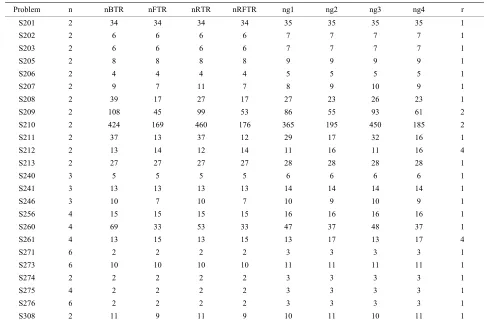
We choose 24 test problems from [29], where “S201” means problem 201 in Schittkowski (1987) collection [29], 12 test problems from CUTE [25,30] and the fa-mous Extended Rosenbrock test problem. In the follow-ing tables, “n” means the test problem’s dimension, “nBTR, nFTR, nRTR, nRFTR” mean the number of it-erations of the algorithm BTR, the algorithm FTR, the algorithm RTR and the algorithm RFTR, respectively. “ng1, ng2, ng3, ng4” mean the number of gradient evaluations of the algorithm BTR, the algorithm FTR, the algorithm RTR and the algorithm RFTR, respec-tively.
“r” means the rank of the number of iterations of the algorithm RFTR among the four algorithms, whose val-ues is in {1, 2, 3, 4}, where “1” means that the number of iterations of the algorithm RFTR is the smallest among the four algorithms, so the algorithm RFTR is the best one among the four algorithms. “4” means that the num-ber of iterations of the algorithm RFTR is the largest among the four algorithms, so the algorithm RFTR is the worst one among the four algorithms. “F” means that the algorithm does not stop when the maximal iteration number is achieved.
Table 1. Reports the numerical results on 24 test problems from [29].
Problem n nBTR nFTR nRTR nRFTR 1ng 2ng 3ng 4ng r
S201 2 34 34 34 34 35 35 35 35 1
S202 2 6 6 6 6 7 7 7 7 1
S203 2 6 6 6 6 7 7 7 7 1
S205 2 8 8 8 8 9 9 9 9 1
S206 2 4 4 4 4 5 5 5 5 1
S207 2 9 7 11 7 8 9 10 9 1
S208 2 39 17 27 17 27 23 26 23 1 S209 2 108 45 99 53 86 55 93 61 2 S210 2 424 169 460 176 365 195 450 185 2 S211 2 37 13 37 12 29 17 32 16 1 S212 2 13 14 12 14 11 16 11 16 4 S213 2 27 27 27 27 28 28 28 28 1
S240 3 5 5 5 5 6 6 6 6 1
S241 3 13 13 13 13 14 14 14 14 1 S246 3 10 7 10 7 10 9 10 9 1 S256 4 15 15 15 15 16 16 16 16 1 S260 4 69 33 53 33 47 37 48 37 1 S261 4 13 15 13 15 13 17 13 17 4
S271 6 2 2 2 2 3 3 3 3 1
S273 6 10 10 10 10 11 11 11 11 1
S274 2 2 2 2 2 3 3 3 3 1
S275 4 2 2 2 2 3 3 3 3 1
S276 6 2 2 2 2 3 3 3 3 1
[image:8.595.53.540.94.416.2]S308 2 11 9 11 9 10 11 10 11 1
Table 2. Reports the numerical results on the famous Extended Rosenbrock test problem.
n nBTR nFTR nRTR nRFTR ng 21 ng 3ng 4ng r
Table 3. Reports the numerical results on 12 test problems from CUTE [25,30].
Problem n nBTR nFTR nRTR nRFTR ng 21 ng 3ng 4ng r
ARHEAD 100 5 5 5 5 6 6 6 6 1
CHN
ROSNS 50 66 39 100 39 51 46 98 46 1
COSINE 100 F F 34 36 986 1008 32 40 2
DQDRTIC 100 4 4 4 4 5 5 5 5 1
ERRINROS 50 52 67 48 27 39 78 44 33 1
FLERCHCR 100 29 29 29 29 30 30 30 30 1
LIARWHD 300 13 13 13 13 14 14 14 14 1
LOGHAIRY 2 61 64 55 31 51 66 50 33 1
NONDIA 100 24 24 24 24 25 25 25 25 1
LS 4
PFIT 3 271 291 309 233 217 323 300 245 1
POWELLS 4 15 15 15 15 16 16 16 16 1
WOOD 4 69 33 53 33 47 37 48 37 1
show that the number for the algorithm RFTR to solve trust region subproblem is the smallest in total.
In Table 2, There are only 2 cases whose rank is sec-ond, the others all are the best. Moreover, the algorithm RFTR is more and more effective as the increase of the problem’s dimension.
In Table 3, There are only 1 case whose rank is second, the others all are the best. Moreover, The retrospective idea takes effects on the Problems COSINE, ERRINROS, LOGHAIRY clearly.
7. Conclusions and Perspectives
Trust region method is very reliable and robust and has very strong convergence properties. It is a class of very effective algorithms for solving unconstrained optimiza-tion now. The basic trust region algorithm is the mono-tone descent algorithm, i.e., the value of the object func-tion in the iterate sequence
xk strictly decreasesmonotonically. If the iterates follow the bottom of curved narrow valleys, then the monotone descent algorithm converges very slowly. The idea of non-monotone method [23,24] abandons the restriction of the descent property of the value of the object function, which allows the sequence of iterates to follow the bottom of curved narrow valleys much more loosely, which hopefully re-sults in longer and more efficient steps.
Trust region method combines with the filter tech-nique, which, in some sense, relaxes the monotonicity condition which accepts the trial step. The filter tech-nique improves the numerical effect for some problems.
The new algorithm RFTR presented in this paper com-bines with the filter technique and the retrospective idea, which the number of the algorithm RFTR to solve trust
region subproblem is decreased in total. On the other hand, our algorithm also looks like a self-adaptive method based on the trust-region framework. Meanwhile, our algorithm is not like the other algorithms about self-adaptive method [26,27] which need to compute the gradient value and function value at the auxiliary point, but may measure the acceptance of the previous iterate and the current iterate for the new and old model func-tion, respectively, which keep the robustness property of the trust-region method.
8. References
[1] M. J. D. Powell, “A New Algorithm for Unconstrained Optimization,” In: J. B. Rosen, O. L. Mangasarian and K. Ritter, Eds., Nonlinear Programming, Academic Press, New York, 1970.
[2] K. Levenberg, “A Method for The Solution of Certain Nonlinear Problems in Least Squares,” The Quarterly of Applied Mathematics, Vol. 2, No. 2, 1944, pp. 164-168. [3] D. W. Marquardt, “An Algorithm for Least Squares
Es-timation of Nonlinear Inequalities,” SIAM Journal on Applied Mathematics, Vol. 11, No. 2, 1963, pp. 431-441. [4] M. J. D. Powell, “Convergence Properties of a Class of
Minimization Algorithms,” In: O. L. Mangasarian, R. R. Meyer and S. M. Robinson, Eds., Nonlinear Program-ming, Academic Press, New York, 1975, pp. 1-27. [5] M. J. D. Powell, “On the Global Convergence of Trust-
Region Algorithms for Unconstrained Optimization,”
Mathematical Programming, Vol. 29, No. 3, 1984, pp. 297-303.
[7] D. C. Sorensen, “Newton’s Method with a Model Trust Region Modifications,” SIAM Journal on Numerical Analysis, Vol. 19, No. 2, 1982, pp. 409-426.
[8] J. J. Moŕe, “Recent Developments in Algorithms and Software for Trust Region Methods,” In A. R. Bachem, M. Grotshel and B. Korte, Eds., Mathematical Program-ming: The State of the Art, Springer-Verlag, Berlin, 1983, pp. 258-287.
[9] Y. X. Yuan, “On the Convergence of Trust Region Algo-rithm,” Mathematica Numerica Sinica, Vol. 16, No. 3, 1996, pp. 333-346.
[10] M. Lalee, J. Nocedal and T. Plantenga, “On the Implenta-tion of an Algorithm for Large-Scale Equality Con-strained Optimization,” SIAM Journal on Optimization, Vol. 8, No. 3, 1998, pp. 682-706.
[11] A. Friedlander, J. M. Martinez and S. A. Santos, “A New Trust Region Algorithm for Bound Constrained Minimi-zation,” Applied Mathematics and Optimization, Vol. 30, No. 3, 1994, pp. 235-266.
[12] A. R. Conn, N. I. M. Gould and P. L. Toint, “Conver-gence Properties of Minimization Algorithms for Convex Constraints Using a Structured Trust Region,” SIAM Journal on Optimization, Vol. 6, No. 4, 1996, pp. 1059- 1086.
[13] A. R. Conn, N. I. M. Gould and P. L. Toint, “Trust Re-gion Methods,” MPS-SIAM Series on Optimization, SIAM, Philadelphia, 2000.
[14] R. Fletcher and S. Leyffer, “Nonlinear Programming without a Penalty Function,” Mathematical Programming, Vol. 91, No. 2, 2002, pp. 239-269.
[15] R. Fletcher, N. I. M. Gould, S. Leyffer, P. L. Toint and A. Wächter, “Global Convergence of a Trust-Region SQP- Filter Algorithm for General Nonlinear Programming,”
SIAM Journal on Optimization, Vol. 13, No. 3, 2002, pp. 635-659.
[16] R. Fletcher, S. Leyffer and P. L. Toint, “On the Global Convergence of a Filter-SQP Algorithm,” SIAM Journal on Optimization, Vol. 13, No. 1, 2002, pp. 44-59. [17] M. Ulbrich, S. Ulbrich and L. N. Vicente, “A Globally
Convergent Primal Dual Interior-Point Filter Method for Nonconvex Nonlinear Programming,” Mathematical Pro-gramming, Vol. 100, No. 2, 2003, pp. 379-410.
[18] A. Wächter and L. T. Biegler, “Line Search Filter Meth-ods for Nonlinear Programming: Motivation and Global Convergence,” SIAM Journal on Optimization, Vol. 16, No. 1, 2005, pp. 1-31.
[19] A. Wächter and L. T. Biegler, “Line Search Filter Meth-ods for Nonlinear Programming: Local Convergence,”
SIAM Journal on Optimization, Vol. 16, No. 1, 2005, pp. 32-48.
[20] R. Fletcher, S. Leyffer and P. L. Toint, “A Brief History of Filter Methods,” SIAG/OPT Views and News, Vol. 18, No. 1, 2006, pp. 2-12.
[21] N. I. M. Gould, C. Sainvitu and P. L. Toint, “A Filter- Trust-Region Method for Unconstrained Optimization,”
SIAM Journal on Optimization, Vol. 16, No. 2, 2005, pp. 341-357.
[22] W. H. Miao and W. Y. Sun, “A Filter Trust-Region Method for Unconstrained Optimization,” Numerical
Mathematics − A Journal of Chinese Universities.
Gaodeng Xuexiao Jisuan Shuxue Xuebao, Vol. 29, No. 1, 2007, pp. 88-96.
[23] L. Grippo, F. Lampariello and S. Lucidi, “A Non-monotone Line Search Technique for Newton’s Meth-ods,” SIAM Journal on Numerical Analysis, Vol. 23, No. 4, 1986, pp. 707-716.
[24] P. L. Toint, “Non-Monotone Trust-Region Algorithms for Nonlinear Optimization Subject to Convex Constraints,”
Mathematical Programming, Vol. 77, No. 1, 1997, pp. 69-94.
[25] F. Bastin, V. Malmedy, M. Mouffe, P. L. Toint and D. Tomanos, “A Retrospective Trust-Region Method for Unconstrained Optimization,” Mathematical Program-ming, Vol. 123, No. 2, 2010, pp. 395-418.
[26] A. Sartenaer, “Automatic Determination of an Initial Trust Region in Nonlinear Programming,” SIAM Journal on Scientific Computing, Vol. 18, No. 6, 1997, pp. 1788- 1803.
[27] X. S. Zhang, Z. W. Chen and J. L. Zhang, “A Self-Adap-tive Trust Region Method Unconstrained Optimization,”
Operations Research Transactions, Vol. 5, No. 1, 2001, pp. 53-62.
[28] N. I. M. Gould, D. Orban, A. Sartenaer and P. L. Toint, “Sensitivity of the Trust-Region Algorithms to Their Pa-rameters,” 4OR: A Quarterly Journal of Operations Re-search, Vol. 3, No. 3, 2005, pp. 227-241.
[29] K. Schittkowski, “More Test Examples for Nonlinear Programming Codes,” Lecture Notes in Economics and Mathematical Systems, Springer Verlag, Berlin, Heide-berg, Vol. 282, 1987.
![Table 3. Reports the numerical results on 12 test problems from CUTE [25,30].](https://thumb-us.123doks.com/thumbv2/123dok_us/8982781.394441/9.595.60.538.94.290/table-reports-numerical-results-test-problems-cute.webp)
