Parameter identification through mode isolation for reaction diffusion systems on arbitrary geometries

(1)

c

The Author(s)

DOI: 10.1142/S1793524518500535

Parameter identiﬁcation through mode isolation for reaction–diﬀusion systems on arbitrary geometries

Laura Murphy

School of Mathematical and Physical Sciences University of Sussex, Department of Mathematics

Brighton BN1 9QH, UK [email protected]

Chandrasekhar Venkataraman School of Mathematics and Statistics University of St Andrews, St Andrews, UK

Anotida Madzvamuse

School of Mathematical and Physical Sciences University of Sussex, Department of Mathematics

Brighton BN1 9QH, UK [email protected]

Received 1 June 2017 Accepted 14 March 2018

Published 3 May 2018

We present a computational framework for isolating spatial patterns arising in the steady states of reaction–diﬀusion systems. Such systems have been used to model many nat-ural phenomena in areas such as developmental and cancer biology, cell motility and material science. In many of these applications, often one is interested in identifying parameters which will lead to a particular pattern for a given reaction–diﬀusion model. To attempt to answer this, we compute eigenpairs of the Laplacian on a variety of domains and use linear stability analysis to determine parameter values for the system that will lead to spatially inhomogeneous steady states whose patterns correspond to particular eigenfunctions. This method has previously been used on domains and sur-faces where the eigenvalues and eigenfunctions are found analytically in closed form. Our contribution to this methodology is that we numerically compute eigenpairs on arbitrary domains and surfaces. Here we present examples and demonstrate that mode isolation is straightforward especially for low eigenvalues. Additionally, we show that in some cases the inhomogeneous steady state can be a linear combination of eigenfunctions. Finally,

This is an Open Access article published by World Scientiﬁc Publishing Company. It is distributed under the terms of the Creative Commons Attribution 4.0 (CC-BY) License. Further distribution of this work is permitted, provided the original work is properly cited.

Int. J. Biomath. 2018.11. Downloaded from www.worldscientific.com

(2)

we show an example suggesting that pattern formation is robust on similar surfaces in cases that the surface either has or does not have a boundary.

Keywords: Reaction–diffusion systems; finite elements; parameter identification; eigen-value problem.

Mathematics Subject Classiﬁcation 2010: 35K55, 37C75, 65M60

1. Introduction

In his seminal work, Turing [59] presented an elegant mathematical theory of reaction–diffusion type for pattern formation in developmental biology. He showed that, via a symmetry breaking process, a homogeneous steady state which is lin-early stable in the absence of diffusion may be driven unstable in the presence of diffusion to give rise to the emergence of a spatially inhomogeneous pattern. This process is now well known asdiffusion-driven instabilityorTuring instability. Since then, reaction–diffusion systems have been proposed and applied to model many natural phenomena including cancer invasion and angiogenesis in cancer biology [10, 11, 21], pattern formation in developmental biology [29, 42], wound healing in biomedicine [13, 52], cell motility [22, 43, 44] and material science [9, 33], among many others. Despite their numerous applications, Turing’s theory of pattern for-mation has been widely criticized mainly due to the lack of robustness of the model system to changes in the parameters as well as the lack of experimental evidence of the existence of so-called morphogens with varying diffusivities. Only recently has the existence of chemical morphogens been experimentally validated in hair follicle pattern formation by Sicket al.[53].

To-date mode selection and parameter identification for reaction–diffusion sys-tems have been mainly carried out on regular planar domains and surfaces where the eigenvalue problem can be analytically solved to yield analytical forms of the wave numbers as well as their corresponding eigenfunctions [22, 36, 41]. In this work, we will depart from this framework and extend computationally mode selection and parameter identification to include arbitrary domains and stationary surfaces. First, we will solve the eigenvalue problem numerically using finite elements on planar domains or surface finite elements on smooth surfaces, respectively, to obtain the eigenmodes and their corresponding eigenfunctions. Here, we employ the Krylov– Schur algorithm [55] for solving the resulting algebraic system arising from the finite element discretization. Second, we then pick an eigenmode to which we apply the necessary and sufficient conditions for Turing diffusion-driven instability in order to isolate reaction-kinetic model parameter values within a reaction–diffusion system. This process can be loosely thought of as an inverse problem for model parameter identification. Once the parameter values are isolated, the full reaction–diffusion system is then solved with these isolated parameter values to obtain an inhomoge-neous spatially varying solution which is then compared to the numerically com-puted eigenfunction on the domain or surface. Alternatively, one could pose the following problem to which this methodology will provide insightful information

(3)

which is otherwise out of reach with the current methodology: Given a biological pattern on a domain or surface and a plausible reaction–diﬀusion system, what are the model parameter values within this reaction–diﬀusion system that will give rise to the observed pattern? This paper provides a theoretical and computational framework to answer such a question. A recent paper by Dhillon et al. [14] uses a similar approach to model pattern development and presents a multiresolution algorithm for tracing bifurcation branches.

It must be observed that the eigenvalue problem and the reaction–diffusion system are both solved by a similar numerical method, the finite element method in multi-dimensions [30]. The finite element method is well known for its capability to deal with complex irregular geometries [6, 18, 60]. Alternative numerical methods such as finite differences [7], spectral methods [11, 50] and finite volume methods among others could be used but with considerable efforts in dealing with geometrical complexities. As mentioned above one interpretation of our approach is that it provides a means of estimating parameter values such that the pattern predicted by linear stability analysis is close to a desired pattern. It must be noted that in many cases the steady state pattern may not be an eigenfunction (or a linear combination of the eigenfunctions) of the Laplacian on the given domain. This is since the nonlinear terms play a role in the resultant steady state pattern [47]. In such a setting our approach may provide parameters which serve as a suitable initial guess for a more advanced parameter identification algorithm [12, 20].

The remainder of this paper is structured as follows. In Sec. 2, we introduce the mathematical model which we study in this work. We summarize the necessary and sufficient conditions for Turingdiffusion-driven instabilityin Sec. 3. We then detail how mode selection and parameter identification are carried out. In Secs. 4 and 6, we outline the new theoretical and computational framework for mode selection and parameter identification. The use of the finite element method is described in Sec. 5. We then give specific examples in 2- and 3-dimensions for regular (by which we mean domains on which analytic expressions for the eigenfunctions are available) as well as general domains and surfaces (where no analytical solutions exist). We discuss the implications of our framework in the context of current methodologies and conclude that given a biological pattern and a reaction–diffusion system, our approach provides a useful tool for estimating parameter values which may give rise to the observed pattern.

2. Mathematical Model Framework

In order to illustrate with clarity the novelty of our approach, we first introduce the standard theoretical framework for reaction–diffusion systems in multi-dimensions [47]. Let Ω⊂Rm₍_m_{= 1}_,₂_,_{3) be a simply connected bounded stationary volume for} all timet∈I = [0, t_F], t_F >0 and ∂Ω be the surface boundary enclosing Ω. Also let u = (u(x, t), v(x, t))T _{be a vector of two chemical concentrations at position} x∈Ω⊂Rmand timet∈I. The evolution equations for reaction–diffusion systems

(4)

in the absence of cross-diﬀusion can be obtained from the application of the law of mass conservation and the extended Fick’s ﬁrst law [47, 59] to yield the dimensional system

            

u_t=D_u∆u+f(u, v),

v_t=D_v∆v+g(u, v), x∈Ω, t >0,

n· ∇u=n· ∇v= 0, xon∂Ω, t≥0,

u(x,0) =u₀(x) and v(x,0) =v₀(x), xon Ω, t= 0,

(2.1)

where ∆ denotes the usual Cartesian Laplace operator, D_u >0 and D_v > 0 are diﬀusion coeﬃcients. Here, nis the unit outward normal to∂Ω. Initial conditions are prescribed through non-negative bounded functions u₀(x) and v₀(x). In the above,f(u, v) andg(u, v) represent nonlinear reactions.

In the case of surfaces, the Laplace operator is replaced by the Laplace–Beltrami operator ∆_Γ, where Γ is the (smooth) surface. Surface gradients are also employed. This can be described as follows (for further details we refer the interested reader to see [16]). If f : Γ → R is diﬀerentiable at x ∈ Γ we can deﬁne the tangential gradient off atx∈Γ by

∇Γf =∇f¯− ∇f¯·nn. (2.2)

Here ¯f is a smooth extension off : Γ→Rto an (n+ 1)-dimensional neighborhood U of the surface Γ, so that ¯f|_Γ =f.∇ is the gradient in Rn+1 _and_n _{is the unit} normal. The Laplace–Beltrami operator applied to a twice diﬀerentiable function f ∈C2(Γ) is then deﬁned by

∆_Γf =∇_Γ· ∇_Γf. (2.3)

It must be observed that if the surface does not have a boundary, no boundary conditions are needed. If the surface has a boundary, we assume homogeneous Neumann boundary conditions.

Since the reaction terms are nonlinear, analytical solutions cannot normally be obtained. Therefore, we investigate solution behavior using linear stability theory and numerical methods. Linear stability analysis is one way of determining the behavior of a nonlinear system near a given stationary point, normally a uniform steady state, of the given system. The idea is to find under what conditions on the nonlinear reaction kinetics is the uniform steady state linearly asymptotically stable in the absence of diffusion. When diffusion is introduced, the uniform steady state is driven unstable in what is now known as the process ofdiffusion-driven instability with the system converging to a spatially inhomogeneous steady state, thereby giving rise to patterning [47, 59]. The mathematical treatment of the derivation of the necessary conditions for diffusion-driven instability requires solving the well-known eigenvalue problem, withW a solution of

∆W +k2W = 0, x∈Ω, (2.4a)

(n· ∇)W = 0, x∈∂Ω, (2.4b)

(5)

where the solution pairs (k (eigenvalues), W_k(x) (eigenfunctions) are obtained either analytically on certain spatial domains or numerically for the general case) of this equation can be compared to the spatially inhomogeneous steady state solu-tions of (2.1), with good agreement expected near primary bifurcation points.

This approach is generally called mode isolation. The most famous exploration of this problem is the celebrated paper “Can one hear the shape of the drum?” by Kac [31]. The question being asked is if one knows all the eigenvalues of the eigenvalue problem is it possible to determine the domain? It was later proven by Gordonet al.[25] that the answer is no and they gave examples of distinct regions with identical eigenvalues.

Other work concerned with mode isolation and linear stability theory for reaction–diffusion systems can be found in [11, 36], here the validation has been mainly restricted to special domains and volumes where the eigenvalue problem can be solved analytically. In this work, we will depart from this framework, instead we will compute approximations of the eigenpairs on arbitrary, simply connected domains, volumes and surfaces. We then use these eigenvalues to calculate, by use of the Turing-parameter space restrictions, appropriate model parameter values. This approach can be thought to be analogous to an inverse parameter identification approach whereby, given the eigenvalues and eigenfunctions solving the eigenvalue problem (2.4), find model parameter values that would give rise to an inhomo-geneous spatially varying solution similar to that exhibited by the eigenfunction. To confirm numerical predictions, we use the computed model parameter values to solve the full nonlinear reaction–diffusion systems and compare approximated eigenfunctions on these arbitrary domains, volumes and surfaces to the spatially inhomogeneous solutions obtained numerically.

To proceed, next we show the two-component form which we will work with and state the conditions fordiﬀusion-driveninstability. These will help us to isolate particular modes.

3. Conditions for Diﬀusion-Driven Instability for Reaction–Diﬀusion Systems

All two-component reaction–diﬀusion systems of the form (2.1) can be non-dimensionalized and scaled to take the form

u_t=γf(u, v) + ∆u, v_t=γg(u, v) +d∆v, x∈Ω⊂Rn, t∈[0,∞], (3.1a)

(n· ∇)

u

v

= 0, x∈∂Ω, t∈[0,∞], (3.1b)

u(x,0), v(x,0) given, (3.1c)

where u = u(x, t), v = v(x, t), d is the ratio of diffusion coefficients, f(u, v) and g(u, v) describe the reaction kinetics. For simplicity, we assume that f and gare continuously differentiable,γ can be described as the relative strength of the

(6)

reaction terms or alternatively as proportional to the domain size. We have zero flux boundary conditions (homogeneous Neumann) because we want only internal sources of instability, i.e. self-organization of the system. A uniform steady state (u_s, v_s) is a fixed point where (u, v) = (u_s, v_s), constant in time and space, sat-isfies (3.1), i.e. (u_t, v_t)|_u₌_u_s_,v₌_v_s = 0. We can find the steady state by solving f(u_s, v_s) =g(u_s, v_s) = 0.

The conditions for instability due to diﬀusion are well known (see, for example, [47]). First, in the absence of diﬀusion, the steady state (u_s, v_s) is linearly stable if and only if the partial derivatives off andg at (u_s, v_s) satisfy

f_u+g_v<0 and f_ug_v−f_vg_u>0. (3.2)

Linear stability analysis considering small perturbations from the equilibrium w(x, t) = (ˆu(x, t),ˆv(x, t)) leads us to the system

w_t=γ

f_u f_v

g_u g_v

w+

1 0

0 d

∆w, (3.3)

which can be solved by method of separation of variables to yield

w(x, t) =

k

c_keλtW_k(x), (3.4)

whereW_k(x) solves the eigenvalue problem

∆W +k2W = 0, x∈Ω, (3.5a)

(n· ∇)W = 0, x∈∂Ω. (3.5b)

These are modes that will decay with time unless the wavenumberk2 satisﬁes

c(k2) =d(k2)2−γ(df_u+g_v)k2+γ2(f_ug_v−f_vg_u)<0, (3.6)

this means that instability will occur if

df_u+g_v >0, (df_u+g_v)2−4d(f_ug_v−f_vg_u)>0 (3.7)

andk2lies in the rangek2₋< k2< k₊2 where

k2_±=γ(dfu+gv)± (dfu+gv)2−4d(fugv−fvgu)

2d . (3.8)

We exploit this range to isolate particular patterns/modes. The unstable modes will correspond to the eigenfunctions of the Laplacian (or Laplace–Beltrami operator) on the chosen domain or surface with the selected boundary conditions andk2 the associated eigenvalues. The eﬀect of varyingdandγon (3.6) is shown in Fig. 1.

In summary the necessary conditions for diﬀusion driven instability are

f_u+g_v <0, f_ug_v−f_vg_u>0, (3.9a)

df_u+g_v >0, (df_u+g_v)2−4d(f_ug_v−f_vg_u)>0. (3.9b)

Additionally, the suﬃcient conditions for patterning formation are that one must be able to isolate distinct real wave numbers and that the domain must be large enough [39, 40, 47].

(7)

[image:7.595.49.398.65.209.2]

(a)γ= 15 (b)d= 10

Fig. 1. Here the dispersal relation (3.6) is plotted (for Schnakenberg kinetics). For a ﬁxed value ofγ, whendis below the critical valuedc,c(k2_{) has no roots so no modes can be isolated. As}_d

increases, so does the diﬀerence between the two roots hence there is more chance that the value ofkwe seek will be betweenk2₋andk+2. Similarly, for a ﬁxed value ofd, increasingγcauses both

k2₋andk+2 to increase.

3.1. Examples of reaction kinetics

For illustrative purposes, we consider three classical reaction kinetics as summarized below. The work presented in this paper holds true for other similar reaction kinetics capable of generating Turing patterns.

3.1.1. Schnakenberg or activator-depleted substrate kinetics

The Schnakenberg kinetics [51] are a condensed version of the well-documented Brusselator model describing a series of autocatalytic reactions also known as activator-depleted models [23, 49], and these are characterized by

AX, B→Y, 2X+Y →3X. (3.10)

Using the law of mass action and the non-dimensionalization of f and g, within system (3.1), we obtain that

f(u, v) =a−u+u2v and g(u, v) =b−u2v, (3.11)

whereaandbare positive parameters.

3.1.2. Gierer–Meinhart kinetics

One of the models proposed by Gierer and Meinhardt [23] describes a system whereby an “activator” activates the production of an “inhibitor” which inhibits the production of the activator. Again the non-dimensionalized form can be obtained

f(u, v) =a−bu+ u 2

v(1 +ku2) and g(u, v) =u

2₋_v, _(3.12)

(8)

where aandb are positive parameters (representing constant production rate and linear degradation rate, respectively) and k can be thought of as the saturation concentration ofu.

3.1.3. Thomas kinetics

The Thomas model [58] is an immobilized-enzyme substrate-inhibition mechanism which can be written in non-dimensional form as

f(u, v) =a−u− ρuv

1 +u+Ku2, g(u, v) =αb−αv−

ρuv

1 +u+Ku2, (3.13)

where a,ρ,K,α,β are all non-negative parameters. This can be interpreted as in [46] by saying that u and v: (i) are generated by constant production a and αb, respectively, (ii) decay linearly proportional touandαv, respectively and (iii) are used up in a substrate inhibition manner ₁₊_uρuv₊_Ku2.

4. Overview on Mode Isolation for Reaction–Diﬀusion Systems

The goal of mode isolation is to choose parameters, in our case (d, γ), so that a trajectory starting from a small random perturbation from the steady state will evolve into a spatial pattern generated by one that corresponds, or at least is close to, a chosen eigenfunction of the Laplacian on that domain. Wavenumber isolation of reaction–diﬀusion systems is described in one dimension, squares and triangles in [36]. In [22], wavenumbers of a visco-elastic model are isolated on the unit disk. We use similar ideas in this work. The basic steps are as follows.

(1) Determine a subset of eigenpairs of the Laplacian with suitable boundary con-ditions on the domain. For special domains this can be done analytically but in general must be done numerically.

(2) Compute the dispersal relation (3.6) for the chosen reaction kinetics (this is independent of the geometry) and the range of admissible wave numbers as a function ofdandγ.

(3) Compute d∗ and γ∗ such that only one of the eigenvalues (wave numbers) computed in step (1) lies in the range.

(4) In order to compare with the patterned state, solve the reaction–diﬀusion sys-tem numerically with computed parameter values and compare with the numer-ically computed eigenfunctions.

It is possible to implement the above procedure simply because if a domain is bounded and the boundary is sufficiently regular, the Neumann Laplacian has a discrete spectrum of infinitely many non-negative eigenvalues with no finite accu-mulation point

0< λ₁≤λ₂≤ · · ·, λ_n→ ∞ (4.1)

and this is due to the spectral theorem for compact self-adjoint operators [8, 32, 57].

(9)

The aim is to have an algorithm to ﬁnd the parameter valuesdandγfor a given eigenpair (k2, W) such that only patterns analogous toW will grow. For this, one needs that the correspondingkis in the range deﬁned in (3.8)

γL=k₋2 < k2< k2₊=γR, (4.2)

where

L= (dfu+gv)− (dfu+gv)2−4d(fugv−fvgu)

2d , (4.3a)

R= (dfu+gv) + (dfu+gv)

2₋₄_d₍_f_u_g_v₋_f_v_g_u₎

2d , (4.3b)

and that no other klies in this range. In other words, the sign of the polynomial c(k2) for a givenk determines if the mode will grow. Figure 1 illustrates how the graph ofc(k2) changes asdandγ are varied. We deﬁne the critical diﬀusion ratio d_c as the root of

d2_cf_u2+ 2(2f_vg_u−f_ug_v)d_c+g2_v= 0. (4.4)

We ﬁnd (k2, W) either analytically or numerically. Then we propose the following algorithm described in pseudo-code:

Input:d=d_c+,≈d_c/5,γ >0,f, g and the k_l,n that we wish to be uniquely

isolated.

(1) Computek2₋ andk2₊ from (4.2).

(2) If k_l,n2 < k2₋ increase γ by 1 (this number is arbitrary but should be small). This moves the curve to higher values ofk.

(3) Ifk_l,n2 < k₊2 decreaseγ by 1. This moves the curve to lower values ofk. (4) If there exists anotherk∗_l,n=k_l,n such thatk₋2 < k_l,n∗2 < k2₊ then decreaseby

d_c/100. This shifts the curve upward so the diﬀerence between k₋2 and k2₊ is smaller.

(5) Ifk_l,n is uniquely isolated END. If not go to (3).

Output:The appropriated, γ.

Note that we cannot haved < d_c (because thenc(k2) would have no roots) nor γ <0 (becausek2>0).

5. Finite Element Method for Reaction–Diﬀusion Systems

In order to validate that our mode isolation algorithm does indeed isolate the desired unstable mode, we will simulate the reaction–diﬀusion systems under consideration with the computed parameter values. To do this we employ a ﬁnite element method for the space discretization and an implicit–explicit time-stepping scheme for the temporal approximation [35, 37, 50].

(10)

In order to compute a ﬁnite element approximation, we write the weak formula-tion of (3.1) as follows: Findu, v∈L2(0, T;H1(Ω)) such that for allφ, ψ∈H1(Ω) we have          Ω u_tφ+

Ω∇

u· ∇φ=γ

Ω

f(u, v)φ,

Ω

v_tψ+d

Ω∇

v· ∇ψ=γ

Ω

g(u, v)ψ,

x∈Ω, t >0. (5.1)

In this work, we shall assume the well posedness of the weak formulation above. We note that for suitable parameter values existence and uniqueness of a classical solution, and hence a weak solution, to (3.1) may be shown for example by the method of invariant regions proposed and analyzed by Sm¨oller [54].

5.1. Spatial discretization

We define the computational domain Ω_h by requiring that Ω_h be a polyhedral approximation to Ω. Furthermore, we defineT_hto be a triangulation of Ω_hmade up of non-degenerate elementsκ_i, i.e.T_h=_i{κ_i}. Finally, we define the finite element spaceV_h:={v_h∈C0(Ω_h) :v_h|_κis linear}. The semidiscrete (space discrete) finite element approximation to (5.1) seeks a pair (U, V)∈V_h2 such that

         Ωh

U_tφ+

Ωh

∇U· ∇φ=γ

Ωh

I_h[f(U, V)]φ,

Ωh

V_tψ+d

Ωh

∇V · ∇ψ=γ

Ωh

I_h[g(U, V)]ψ,

∀φ, ψ∈V_h, (5.2)

where we use the Lagrange interpolant I_h of the initial data into V_h as initial conditions for the scheme. LettingN_hbe the total number of degrees of freedom of the nodes for the ﬁnite element discretization, we can write

U = Nh

i=1

α_iφ_i, V = Nh

i=1

β_iφ_i, whereφ_i(xj, t)∈V_h:φ_i=

1 ifi=j,

0 ifi=j. (5.3)

In order to illustrate a concrete example of the scheme, we focus on the reaction– diﬀusion system with Schnakenberg kinetics (3.11). The ﬁnite element approxima-tion (5.2) with the Schnakenberg kinetics can be written in matrix-vector form as follows:

Mα_t+Aα=γ[aH−Mα+Mα2β], (5.4a)

Mβ_t+dAβ=γ[bH−Mα2β], (5.4b)

where α = (α₁, . . . , α_N_h) andβ = (β₁, . . . , β_N_h) are the coefficient vectors of the finite element functionsU andV respectively andMandAare mass and stiffness matrices andH is a load vector with entries given by

M_i,j=

Ωh

φ_iφ_j, A_i,j=

Ωh

∇φ_i· ∇φ_j, H_j=

Ωh

φ_j, i= 1, . . . , N_h. (5.5)

(11)

5.2. Temporal discretization

For the temporal discretization we employ an IMEX method [35, 37, 50] in which the diﬀusive term is treated implicitly and the reaction terms are treated explicitly, for simplicity we employ a uniform timestep τ. Introducing the shorthand for a time discrete sequence of functions, fn = f(t_n), the fully discrete scheme we employ reads, for n = 0,1, . . . , given (Un_{, V}n₎ _∈ _V2

h ﬁnd (Un+1, Vn+1) ∈ Vh2 such that, ∀φ, ψ∈V_h,

           Ωh 1 τ(U

n+1₋_Un₎_φ₊

Ωh

∇Un+1· ∇φ=γ

Ωh

I_h[f(Un, Vn)]φ,

Ωh

1 τ(V

n+1₋_Vn₎_ψ₊_d

Ωh

∇Vn+1· ∇ψ=γ

Ωh

I_h[g(Un, Vn)]ψ,

(5.6)

where we use Lagrange interpolant of the initial data intoV_h as initial conditions for the scheme. This leads us to the following matrix vector form:

1 τM+A

αn+1 ₌_γ_[_a_H₋_M_αn₊_M₍_αn₎2_βn_{] +}1

τMα

n_, _(5.7a)

1

τM+dA

βn+1 ₌_γ_[_b_H₋_M₍_αn₎2_βn_{] +} 1

τMβ

n_. _(5.7b)

Since we are interested in convergence to a spatially inhomogeneous steady state, for the stopping criteria we use theL₂norm of the approximate time-derivative of the discrete solution, stopping the computation if this decreases below a tolerance, usually 10−9 (see Fig. 2).

5.3. Numerical computations

We take the parameter values as shown in Table 1, and discretisation parameters as in Table 2. The uniform states for Schnakenberg kinetics were obtained analytically while for the Gierer–Meinhardt and Thomas reaction kinetics these were calculated computationally using the Newton–Raphson method [2, 36]. For the initial data we use small quasi-random perturbations around the uniform steady state values. The linear system (5.7) is solved using the conjugate gradient method [4, 24, 28].

5.4. Convergence to a steady state

[image:11.595.47.397.567.617.2]

Figure 2 plots the L₂ norm of the discrete time-derivative of U and V against the elapsed time. To begin with theL₂ norm is large. This quickly decays due to

Table 1. Parameters for reaction kinetic models and the corresponding uniform steady states.

Model a b k K α ρ us vs

Schnakenberg 0.9 0.1 1 0.9

Gierer–Meinhart 0.1 1 0.5 0.8395 0.7047

Thomas 150 100 0.05 1.5 13 37.74 25.16

(12)

[image:12.595.76.370.76.357.2]

Table 2. Discretization parameters. Time-step ﬁxed as 10−3_.

Domain Type Degrees of freedom No. of cells h

Sphere Volume 3817 3584 0.0915064

Ellipse Area 1313 1280 0.0404632

Dumbbell Volume 29,521 28,672 0.0280245

Sphere surface Surface area 6146 6144 0.0630101

“Fish” Surface 6146 6144 0.00940557

“Eel open” Surface 2112 2048 0.0540314

“Eel closed” Surface 4610 4608 0.00631303

Fig. 2. Plot of theL2 norm of the discrete time-derivative over time for the example shown in

Fig. 8(b). There is an initial decay due to diﬀusion followed by a growth because of the exponen-tially growing modes which eventually decays, due to the dominant nonlinear terms.

diﬀusion followed by a rapid growth, because of the exponentially growing modes. The time-derivative eventually starts to decay due to the eﬀects of the nonlinear terms that act to bind the exponentially growing solution thereby giving rise to a spatially inhomogeneous steady state.

6. Isolating Modes on General Domains

On arbitrary domains, analytical solutions for the eigenvalue problem are not typ-ically available but approximate eigenpairs can be computed numertyp-ically. Numer-ically approximating these pairs is a signiﬁcant challenge. In general, as we are typically interested in a small number of eigenpairs, it is not necessary to ﬁnd all solution pairs, however for our approach to mode isolation to remain applicable, it is important that we obtain consecutive pairs.

As previously stated, the eigenvalue problem we wish to solve is as follows:

∆W+k2W = 0, x∈Ω,

(n· ∇)W = 0, x∈∂Ω. (6.1)

[image:12.595.73.373.81.169.2]

(13)

To approximate the solution we employ the ﬁnite element method for the spatial discretization outlined in Sec. 5. We work with the weak formulation of the eigen-value problem and look for an approximate eigenpairs (W_h, k2_h)∈V_h×R₊ (where V_hcontains all continuous piecewise linear functions on a given mesh) such that

Ω∇

W_h· ∇φ=k2

Ω

W_h·φ, ∀φ∈V_h. (6.2)

As in (5.4) this may be written in matrix-vector form, we want to ﬁnd (w, k2_h)∈

Rm_×_R

+, wheremis the dimension ofV_h such that

Aw=k2Mw, (6.3)

where A and M are stiﬀness and mass matrices deﬁned in the same way as in Eq. (5.5). This is a generalized eigenvalue problem. We use the packagedeal.II[4] for its approximation using SLEPc and the Krylov–Schur algorithm. For complete-ness we give a description of the algorithm employed in Appendix A.

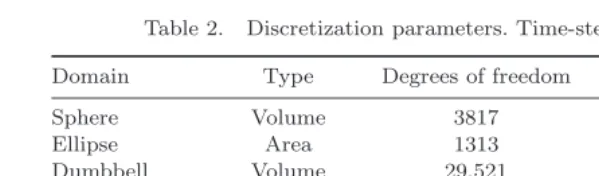
7. Mesh Generation

All the mesh generation is carried out using thedeal.IIlibrary. We use hexahedral meshes for the volumes and quadrilaterals for the ellipse and surfaces. In Fig. 3, we exhibit diﬀerent meshes generated by this package on which we will carry out com-putations. We also consider smooth surfaces; these meshes are generated by creating

(a) Unit sphere (b) Unit sphere cut to show inside

[image:13.595.111.333.358.558.2]

(c) Surface of unit sphere (d) Ellipse

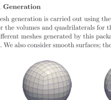
Fig. 3. Examples of mesh generation for diﬀerent volumes and surfaces: (a)–(c) Mesh generation on the unit sphere. (d) The ellipse which is a deformation of a circle mesh. (e)–(f) The dumbbell is a deformation of the bulk of a sphere. (g) The “ﬁsh” shape is a deformation of the surface of a sphere. (h) An “eel” is modeled by a cylinder with an open boundary and additionally as the same cylinder with added rounded boundaries.

(14)

(e) Dumbbell mesh (f) Inner structure of dumbbell mesh

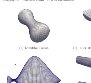
[image:14.595.65.361.63.330.2]

(g) “Fish” mesh (h) “Eel” meshes (with and without boundary) Fig. 3. (Continued)

a triangulation Ω_h of the bulk of the domain Ω then the surface triangulation is deﬁned by collecting the faces of the elements of the bulk triangulation that lie on the surface (Γ_h= Ω_h|_dΩ), i.e. the surface mesh is the trace of the volume mesh (in the example of the cylinder with open ends we use only the elements on the curved surface). For this reason the equations are not being approximated on the actual surface but on an approximation of it. For more details on surface mesh generation the reader is referred to [4] and the references therein.

8. Comparisons of Eigenfunctions and Spatially Inhomogeneous Steady States

8.1. Example 1: Sphere

We start by considering the unit sphere, a domain for which the eigenvalue problem can be solved analytically.

8.1.1. Eigenvalues and eigenfunctions of the Laplacian in the bulk of the unit sphere

In order to solve (2.4) on the sphere, we convert the eigenvalue problem into spheri-cal coordinates. The eigenvalue problem in spherispheri-cal coordinates is as follows [2, 45]:

∆w+k2w= 1 r2

∂ ∂r

r2∂w

∂r

+ 1

r2sinθ ∂ ∂θ

sinθ∂w

∂θ

+ 1

r2sinθ ∂2w ∂φ2 +k

2_w_{= 0}_,

(15)

with homogeneous Neumann boundary conditions. The solutions of the above eigen-value problem are well known and are obtained using separation of variables [2, 45]. Following [2, pp. 424–428] we ﬁnd an inﬁnite number of discrete solutions of the form

wm_l,n(r, θ, φ) =Am_l,nJ_l₊1 2

j_l₊1

2,nr

eimφP_lm(cosθ), (8.1)

where l, m, n are all integers such that |m| ≤ l ≤ n, Am

l,n are constants, Jα(x) is a Bessel function of the ﬁrst kind, i.e. J_α(x) = ∞_j₌₀ (−1)j

j!Γ(1+j+α)( x

2)2j+α with Γ(n) = (n−1)!,P_lm(x) are the associated Legendre polynomials andj

l+12,nare zeros of the diﬀerential of the spherical Bessel function. We can ﬁnd the eigenvaluesk2_l,n= (j

l+1₂,n)2numerically (using the fact thatJl+1₂,n= l

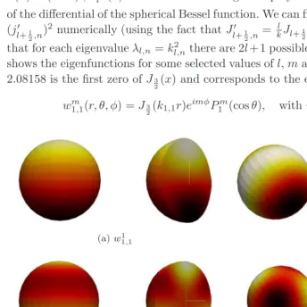
kJl+1₂(k)−Jl+3₂(k)). It follows that for each eigenvalueλ_l,n=k_l,n2 there are 2l+ 1 possible eigenfunctions. Figure 4 shows the eigenfunctions for some selected values ofl,mandn. For examplek₁_,₁= 2.08158 is the ﬁrst zero ofJ3

2(x) and corresponds to the eigenfunctions

w₁m_,₁(r, θ, φ) =J3

2(k1,1r)e imφ_Pm

1 (cosθ), withm=−1,0,1. (8.2)

(a)w1

1,1 (b)w02,1

(c)w0

3,1 (d)w−3,21

[image:15.595.49.393.250.594.2]

(e)w−₄_,3₁

Fig. 4. Analytical solutions to the eigenvalue problem on the unit sphere i.e. (8.1) for selected values ofl,mandn. These are plotted usingdeal.II.

(16)

The spherical Bessel function is given by J3

2(k1,1r) =

sin(k1,1r)

(k1,1r)2 −

cos(k1,1r) k1,1r . Meanwhile Y₁m=eimφP₁m(cosθ) are spherical harmonics whose real parts can be

written in Cartesian coordinates asY₁−1=

3 4π·

y r,Y10=

3

4π·zrandY11=

3 4π·xr. Since the system we are solving is invariant to polarity we can consider these to be equivalent. Figure 4(a) shows a plot of the eigenfunction

w1₁_,₁=

sin(k₁_,₁r) (k₁_,₁r)2 −

cos(k₁_,₁r) k₁_,₁r

·x

r, (8.3)

where as usualr2=x2+y2+z2. The second examplek₂_,₁= 3.34209 corresponds to the eigenfunctions

w₂m_,₁(r, θ, φ) =J5

2(k2,1r)e imφ_Pm

2 (cosθ), with −l≤m≤l. (8.4)

Choosingm= 0, converting the above to Cartesian coordinates and taking the real part gives

w0₂_,₁(x, y, z) =

3 k₂2_,₁r2 −1

sin(k₂_,₁r) k₂_,₁r −

3 cos(k₂_,₁r) k2₂_,₁r2

× 1 4 5 π·

−x2−y2+ 2z2 r2

.

The plot of the functionw0₂₁is shown in Fig. 4(b).

8.1.2. Mode isolation on the sphere

Using the method described in Sec. 4 with all other parameters ﬁxed as in Table 1 we can isolate the wavenumbers for the reaction–diﬀusion system with Schnakenberg kinetics and these are shown in Table 3. Similarly, for Thomas and Gierer–Meinhart (Table 4). In all these cases the interval [k₋, k₊] is centered onk_l,n.

8.1.3. Simulations of the reaction–diﬀusion systems on the unit sphere

[image:16.595.82.365.558.617.2]

Solving usingdeal.IIwe use the mesh shown in Fig. 3(a). The timestep is taken to beτ= 10−3. We take the initial conditions to be a small random perturbation from the previously computed homogeneous steady state. So for the reaction–diﬀusion

Table 3. Given particular values ofdandγwe obtain the values fork−and

k+as well as the corresponding wavenumbers that are isolated on the sphere,

for the reaction–diﬀusion system with Schnakenberg kinetics.

d γ k− k+ Wavenumbers excited

10 15 1.7321 2.7386 k1,1= 2.08158

10 40 2.8284 4.4721 k2,1= 3.34209

9 60 3.9319 5.0866 k0,2= 4.49341,k3,1= 4.51410

8.81 85 4.8575 5.8955 k4,1= 5.64670

(17)

[image:17.595.93.351.91.151.2]

Table 4. The values ofdandγwhich isolate the given wavenumbers on the sphere for the Gierer–Meinhart and Thomas reaction kinetics.

Gierer–Meinhart Thomas Wavenumbers excited

d= 74,γ= 30 d= 30,γ= 15 k1,1

d= 74,γ= 80 d= 30,γ= 40 k2,1

d= 74,γ= 160 d= 28,γ= 60 k0,2,k3,1

d= 72,γ= 200 d= 27.5,γ= 90 k4,1

system with Schnakenberg kinetics, at each point in the grid we set the initial conditions to be

α0= 0.995 + 0.01, β0= 0.895 + 0.01, (8.5)

whereis a uniformly distributed random variable between 0 and 1.

For each eigenvalue there are a number of diﬀerent eigenfunctions. Computing using the values obtained with mode isolation, the solution converges to either one of the eigenfunctions or a linear combination. These converged solutions are shown in Figs. 5 and 6. It is possible to force the solution to converge to an eigenfunc-tion (which it does not appear to with random initial perturbaeigenfunc-tion) by making a suitable choice of initial condition, for example a perturbation of the desired

(a)γ= 15,d= 10 (b)γ= 40,d= 10

(c)γ= 70,d= 9 (d)γ= 85,d= 8.81

Fig. 5. Converged solutions of system (3.1) with Schnakenberg kinetics (3.11). These solutions represent the speciesu. The isolated modes arew1

1,1,w02,1,w03,1andw4−,31.

[image:17.595.49.396.319.591.2]

(18)

(a) Gierer–Meinhart,γ= 80,d= 74 (b) Thomas,γ= 40,d= 30

(c) Gierer–Meinhart,γ= 160,d= 74 (d) Thomas,γ= 70,d= 28

[image:18.595.47.396.62.461.2]

(e) Gierer–Meinhart,γ= 200,d= 72 (f) Thomas,γ= 90,d= 27.5

Fig. 6. Converged solutions of system (3.1) for the speciesuwith Gierer–Meinhart kinetics (3.12) on the left with isolated modesw0

2,1,w33,1andw−4,31and Thomas (3.13) on the right with isolated

modesw02,1,w−3,12andw− 3 4,1.

eigenfunction, suitably scaled. Hence, in the case where multiple wave numbers are excited, pattern selection is heavily inﬂuenced by the choice of initial conditions which act as the basin of attraction, one of the major criticisms of Turing’s theory for pattern formation [5].

8.2. Example 2: Ellipse

Eigenmodes on an ellipse have been investigated in various papers [19, 26, 48, 61]. Finding the solution involves numerically solving the Mathieu and modiﬁed

(19)

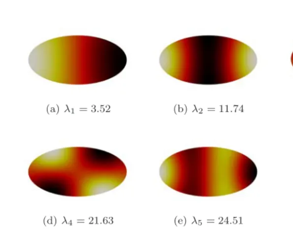
(a)λ1= 3.52 (b)λ2= 11.74 (c)λ3= 12.52

(d)λ4= 21.63 (e)λ5= 24.51 (f)λ6= 34.30

[image:19.595.72.370.72.308.2]

(g)λ7= 41.75 (h)λ8= 45.88 (i)λ9= 50.97

Fig. 7. Eigenfunctions corresponding to the labeled eigenvalues on an ellipse. These are solutions of (6.1) approximated usingdeal.II.

Mathieu equations [1]. In particular Wu and Shivakumar [61] analytically ﬁnd the ﬁrst eigenvalue of ellipses with Dirichlet boundary conditions, of various sizes of ellipse. Using the eigenvalue solver described in Sec. 6, with Dirichlet boundary conditions, we can reproduce their results (results not reported for brevity’s sake). In the following we consider Neumann boundary conditions and choose the semi-major axis to be twice the semi-minor axis.

The eigenvalues and eigenfunctions are shown in Fig. 7. Figure 8 shows the converged solutions of the reaction–diﬀusion system when the chosen values of d andγisolate the corresponding wavenumbersk_i2=λ_i. It must be observed that the pattern computed will be a scalar multiple of the eigenfunction. This scalar may be negative which results in a reversed pattern (compare for example Figs. 7(a) and 7(g) with Figs. 8(a) and 8(g), respectively). Similarly for later examples shown in Figs. 10(e) and 12(c), 12(e) and 12(g).

8.3. Example 3: Dumbbell

As a third example we consider the dumbbell shaped domain shown in Fig. 3(e). The solver for the eigenvalue problem on this mesh gives the output of eigenvalues and eigenfunctions shown in Fig. 9. The corresponding steady state solutions with the parameters obtained by mode isolation are shown in Fig. 10.

(20)

(a)d= 10,γ= 10 (b)d= 8.8,γ= 30 (c)d= 8.8,γ= 44

(d)d= 8.8,γ= 57 (e)d= 8.7,γ= 77 (f)d= 8.7,γ= 95

[image:20.595.79.365.74.308.2]

(g)d= 8.63,γ= 115 (h)d= 8.61,γ= 135 (i)d= 8.61,γ= 150

Fig. 8. Converged solutions of system (3.1) with Schnakenberg kinetics (3.11), on an ellipse for the speciesu, they all match the associated eigenfunctions shown in Fig. 7. It must be noted that the pattern can appear to be reversed (e.g. in (a) and (g)), this is due to the choice of the initial conditions. Choosing appropriate initial conditions results in a pattern similar to that shown in Fig. 7(a) or 7(g).

(a)λ1= 1.49 (b)λ2= 12.68 (c)λ3= 22.86

(d)λ4= 22.98 (e)λ5= 26.52 (f)λ6= 49.91

Fig. 9. Eigenfunctions corresponding to the labeled eigenvalues on the dumbbell. These are solutions of (6.1) approximated usingdeal.II.

[image:20.595.55.397.392.557.2]

(21)

(a)d= 10,γ= 5 (b)d= 9,γ= 40 (c)d= 8.8,γ= 60

[image:21.595.51.396.76.241.2]

(d)d= 8.8,γ= 88 (e)d= 8.65,γ= 130

Fig. 10. Convergedusolutions of system (3.1) with Schnakenberg kinetics (3.11) on a dumbbell. Eigenvaluesλ1, λ2, λ5, λ6have been isolated, however sinceλ3≈λ4in (c) we see a linear

combi-nation of their eigenfunctions. (e) Shows a reversed mode due to the nature of the random initial conditions as previously described in Sec. 8.2.

8.4. Example 4: Surface of a sphere

In all the previous examples we considered bulk, volumetric domains. In this exam-ple we have a curved surface as the domain. This means using the Laplace Beltrami operator ∆_Γinstead of the Laplacian ∆ in (6.1) and (3.1). To approximate solutions in this case, we employ the surface ﬁnite element method [6, 15–18, 38].

The eigenpairs on the surface of the unit sphere can be found analytically and are well known and documented in [11] for example. The eigenfunctions are referred to as spherical harmonics. They are the restrictions of the eigenfunctions (8.1) to the surface. The eigenvalues are of the formk2=l(l+ 1), wherelis an integer, and the eigenfunctions are

wm_l (θ, φ) =Am_l eimφP_lm(cosθ), (8.6)

where m and Pm

l are as described in Sec. 8.1.3. Therefore, we can test the per-formance of the eigenvalue problem solver with this example. Using the eigenvalue solver on an approximated mesh of the surface of the sphere using 98306 degrees of freedom we obtain the following output of the first 30 eigenvalues computed to six significant figures:

k_h2= 2.00009,2.00009,2.00009,6.00042,6.00042,6.00042,6.00053,6.00053,

12.0013,12.0015,12.0015,12.0015,12.0016,12.0017,12.0017,20.003,

20.003,20.0032,20.004,20.0041,20.0042,20.0042,20.0045,20.0046,

30.0066,30.0067,30.0067,30.0068,30.0081,30.0095. (8.7)

(22)

[image:22.595.90.359.68.184.2]

(a) (b)

Fig. 11. Mode isolation for the reaction–diﬀusion system with Schnakenberg kinetics on the surface of the sphere. (a) The surface ﬁnite element solution with given parameters d= 9 and

γ= 35 and (b) numerically computed eigenfunction corresponding to eigenvalueλ9= 12.0186.

As expected these are the first five values of the form k2 = l(l + 1) with l = 1,2,3,4,5. It must be observed that the finite element method is known to be less effective for higher eigenvalues due to the min-max theorem [56]. This means we must use a highly refined mesh in order to obtain values that are closer to the analytical values. The eigenfunctions are analogous to those detailed in Sec. 8.1.3 restricted to the boundary. This shows that the eigenvalue solver gives the required output. Since the results are shown in Sec. 8.1.3, we only show one example of mode isolation in Fig. 11. As mentioned in Sec. 3, γ can be thought of as being proportional to the domain size. Here we only consider a sphere with radius one. As the size of the sphere (radiusR) increases, the eigenvalues decrease (specifically they are multiplied by _R12). This effect is demonstrated in [34] where they show that fixing other values and increasing R causes higher mode patterns and hence more complex patterns are obtained.

8.5. Example 5: “Fish” surface

We now consider a smooth surface on which no analytical expression for the eigen-pairs is available, the surface is taken to be diffeomorphic to the sphere and is shown in Fig. 3(g), it is meant to (very loosely) mimic the shape of a fish. We found the first 100 eigenpairs then chose several to isolate. These are shown in Fig. 12. Various patterns are observed including stripes, spots and concentric rings.

8.6. Examples 6 and 7: “Eel” shapes

When computing on surfaces, one has to consider whether or not the surface has a boundary. In papers modeling ﬁsh or eel patterns (see, for example, [60]), a surface with a boundary is often used. To investigate whether having a boundary is signiﬁcant in this example we consider a surface with and without boundary. We see, in Figs. 13 and 14, that the eigenvalues and eigenfunctions are very similar and it is possible to isolate similar patterns using the same parameter values.

(23)

(a)d= 8.9,γ= 130 (b)λ5= 40.18

(c)d= 8.58,γ= 240 (d)λ10= 79.56

(e)d= 8.58,γ= 400 (f)λ15= 134.73

[image:23.595.90.360.60.565.2]

(g)d= 8.58,γ= 510 (h)λ19= 175.98

Fig. 12. Surface ﬁnite element solutions corresponding to theuspecies of the reaction–diﬀusion system with Schnakenberg kinetics with the given parameters on the left and numerically com-puted eigenfunctions corresponding to the given eigenvalue on the right. Again we observe reversed modes as described in Sec. 8.2.

(24)

(a)λ4(open)= 54.43 (b)λ4(closed)= 44.94

(c)λ23(open)= 253.69 (d)λ25(closed)= 257.54

[image:24.595.123.322.67.275.2]

(e)λ24(open)= 253.73

Fig. 13. Eigenfunctions of the Laplace–Beltrami operator on the “eel” shape with the corre-sponding eigenvalue. The left column shows the surface without a boundary and the right has a boundary. Note that, although the eigenfunctions are diﬀerent,λ23≈λ24.

(a)d= 8.8,γ= 140 (b)d= 8.8,γ= 140

(c)d= 8.6,γ= 750 (d)d= 8.6,γ= 750

Fig. 14. Converged solutions corresponding to theuspecies of the reaction–diﬀusion system with Schnakenberg kinetics on the surface of an eel. The surfaces on the right have a boundary whereas those on the left do not. We ﬁnd that using the same parameter values on both surfaces gives very similar results.

8.7. Quantitative comparisons

By inspecting the plots it can be observed that the modes qualitatively appear to be isolated. To further expand on this, we normalize both the solutions and eigenfunc-tions to be in the range [−1,1] then compute the L2 norm of their diﬀerence and

[image:24.595.84.360.332.504.2]

(25)

[image:25.595.78.367.90.202.2]

Table 5. L2 _{norm of diﬀerence between converged solution and the selected}

eigenfunction (U−ωk) is found for the examples shown.

Ellipse L2 _Dumbbell _L2 _“Fish” _L2

ω1 9.6623×10−3 ω1 0.35029 ω5 0.076100

ω2 9.7404×10−3 ω2 0.034952 ω10 0.015871

ω3 0.028500 ω5 0.020861 ω15 0.010345

ω4 0.037851 ω6 0.010280 ω19 6.9365×10−3

ω5 0.039147

ω6 0.030712

ω7 0.021398

ω8 0.066343

ω9 0.056569

results of these computations are shown in Table 5. Results on the sphere are not possible due to rotational symmetry. It turns out that theseL₂norm differences are small and are due to a number of factors: First, the chosen numerical parameters: the differences get smaller and smaller with further grid refinement. On the other hand, numerical tests seem to suggest that refining the time-step does not make a significant difference in the decrease of theL₂ norms. Second, due to mode clus-tering, theL₂norm differences can be affected by small contributions from nearby modes that are residing in the same excitable region. Last, the treatment of the nonlinear terms plays a significant role in the decrease of theseL₂norm differences.

9. Conclusion and Further Challenges

In this paper, we have considered reaction–diffusion systems and have presented a framework for isolating particular spatially inhomogeneous patterns. The method involves finding eigenpairs of the Laplacian (or more generally Laplace–Beltrami), and computing parameters such that when the reaction–diffusion system is solved numerically, only patterns analogous to a particular eigenfunction will grow. In previous works the eigenvalue problem is solved analytically whereas in this paper both the eigenvalue problem and the reaction–diffusion system are solved using the finite element method. Advances in numerical software mean that we can find 100 eigenpairs in a few minutes and we have demonstrated that these eigenpairs match analytical results. The approach is shown to work for three different examples of nonlinear reaction kinetics and on a variety of domains and surfaces. In summary, the main observations are:

• Mode isolation is straightforward for low values ofk2 but can become slightly more diﬃcult for higher values of k2. This is due to the approximation of the nonlinear terms and clustering of the eigenvalues of the linear problem.

• When two or more eigenvalues are clustered close to each other it becomes diﬃcult to isolate them computationally as well as analyltically. If two or more eigenvalues are in the permissible range then the inhomogeneous steady state could be a linear combination of the corresponding eigenfunctions.

(26)

• We display an example of two surfaces where pattern formation appears to be robust despite the fact one has a boundary while the other does not. An interest-ing investigation would be to see if this can be true for other geometries. Note that this observation is only for the case of zero-ﬂux boundary conditions. Imposing Dirichlet or Robin-type boundary conditions would result in substantially diﬀer-ent patterns.

In this paper, we have only considered stationary domains/volumes and surfaces. However, the domains of biological processes generally evolve with time [6, 18, 35, 37, 60]. This adds more complexity to solving the reaction–diﬀusion systems. An interesting and natural extension of this work would be to introduce domain growth and surface evolution. For this extension, studies on the eﬀects of initial conditions would also be worthwhile.

Data Availability

All relevant data is contained within the manuscript. The computational code used to generate the Figures and Tables in the manuscript is available on request.

Acknowledgments

The authors thank anonymous reviewers for their valuable comments. This work (L. Murphy) was supported by an EPSRC Doctoral Training Centre Studentship through the University of Sussex. C. Venkataraman and A. Madzvamuse acknowl-edge support from the Leverhulme Trust Research Project Grant (RPG-2014-149) and the EPSRC grant (EP/J016780/1). This research was partly undertaken whilst L. Murphy, C. Venkataraman and A. Madzvamuse were participants in the Isaac Newton Institute Program, Coupling Geometric PDEs with Physics for Cell Mor-phology, Motility and Pattern Formation. This work (A. Madzvamuse) has received funding from the European Union Horizon 2020 research and innovation programme under the Marie Sklodowska-Curie grant agreement (No. 642866). A. Madzvamuse was partially supported by a grant from the Simons Foundation. A. Madzvamuse is a Royal Society Wolfson Research Merit Award Holder, generously supported by the Wolfson Foundation. L. Murphy acknowledges the support from the University of Sussex ITS for computational purposes.

Appendix A. The Krylov–Schur Algorithm

The Krylov–Schur algorithm was introduced by [55] and is an alternative to the method of [3]. The aim of the algorithm is to compute a number of eigenpairs of a given square matrix A.

The basicArnoldi algorithm has input matrixA and initial vector v₁ of norm 1 (v_j will make up the columns of ann×mmatrixV_m) and outputV_m,H_m,f, β such that

AV_m=V_mH_m+f e_m∗, β=f₂. (A.1)

(27)

A Krylov decomposition is a generalized version of this and is given by

AV_m=V_mB_m+v_m₊₁b∗_m₊₁, (A.2)

whereB_mis not necessarily upper Heisenberg andb∗_m₊₁is an arbitrary vector. The Krylov–Schur method is described in the SLEPc Technical Report [27] as follows:

Input: MatrixA, initial vectorv₁, and dimension of the subspacem

Output: A partial Schur decompositionAV_1:_k=V_1:_kH_1:_k,_1:_k

• Normalizev₁

• InitializeV_m= [v₁], k= 0, p= 0

• Restart loop

— Performm−psteps of Arnoldi with deﬂation

— ReduceH_m(part of the output of the Arnoldi algorithm) to (quasi-)triangular form,H_m←U∗₁H_mU₁

— Sort the 1×1 or 2×2 diagonal blocks:H_m←U∗₂H_mU₂ — U=U₁U₂

— Compute eigenpairs ofH_m,H_my_i=y_iθ_i — Compute residual norm estimates,τ_i=β|e∗_my_i| — V_m←V_mU

— Exit if enough converged eigenpairs, otherwise lock newly converged vectors — Choose p (k (the number of currently converged eigenpairs)< p < m) and

set ˜v_p₊₁=v_m₊₁

— Computeb_w(the leading subvector ofb∗_m₊₁U) and insert in the appropriate positions ofH_p

• end

If the eigenpairs of H_1:_k,_1:_k (i.e. solutions of Hy = θy) are (θ_i,y_i) then the approximate eigenvalues ofAareλ_i =θ_i and eigenvectors arexi=V_1:_ky_i. In our problem we have (6.3) (the generalized eigenvalue problem) instead ofAx=λx, and here one works with a spectral transformation T_S = M−1A or T_SI = (A−σI)M instead ofA.

References

[1] M. Abramowitz and I. Stegun,Handbook of Mathematical Functions (Dover Publi-cations, New York, 1970).

[2] G. Arfken, H. Weber and F. Harris,Mathematical Methods for Physicists(Elsevier, Amsterdam, 2013).

[3] W. Arnoldi, The principle of minimized iterations in the solution of the matrix eigen-value problem,Quart. Appl. Math.9(1951) 17–29.

[4] W. Bangerth, T. Heister, L. Heltai, G. Kanschat, M. Kronbichler, M. Maier and B. Turcksin, The deal.ii library, version 8.3,Arch. Numer. Softw.4(100) (2016) 1–11.

[5] J. Bard and I. Lauder, How well does Turing’s theory of morphogenesis work?

J. Theor. Biol.45(1974) 501–531.