Dose selection in seamless phase II/III clinical trials based on efficacy and toxicity

(1)

A Thesis Submitted for the Degree of PhD at the University of Warwick

http://go.warwick.ac.uk/wrap/2765

This thesis is made available online and is protected by original copyright. Please scroll down to view the document itself.

(2)

Dose Selection in Seamless Phase II/III Clinical

Trials based on Efficacy and Toxicity

by

Peter Kung’u Kimani

Thesis

Submitted in partial fulfilment of the requirements

for the degree of

Doctor of Philosophy in Statistics

Department of Statistics

(3)

List of Tables

2.1 Simplest decision making problem . . . 15 3.1 Chance of successive treatment failures when probability of success is 0.2 . 33 3.2 Decision boundaries at inspection 1 using Gehan’s method . . . 34 3.3 Cross tabulation of toxicity and efficacy . . . 46 6.1 Probabilities of efficacy and toxicity at tested dose levels for the three

sce-narios used to assess effect of efficacy . . . 103 6.2 Probabilities of efficacy and toxicity at tested dose levels for the three

sce-narios used to assess effect of toxicity . . . 104

(7)

List of Figures

2.1 Beta densities with different parameter values. The legends give the values

of the parameters. . . 8

2.2 Beta curves with same mean (0.2) but different parameter values . . . 10

3.1 Phase I set-up . . . 21

3.2 Flowcharts of the traditional design (Design A) . . . 22

3.3 A variation of the traditional design (Design D) . . . 23

3.4 A phase II setting allowing for 3 actions at each inspection . . . 31

3.5 Range of the parameter values . . . 37

3.6 Possible outcomes at stage(i+ 1) . . . 41

3.7 (a) The preference regions forµ = (µ1, µ2). The first position in the pair correspond toX1 (efficacy) and the second position toX2 (toxicity). The symbols +, 0 and - respectively indicates new drug is preferred, considered equivalent and unacceptable. (b) An example of appropriate actions for specified values ofµ; R (reject new drug) and A (accept new drug) . . . 43

3.8 Dose response curves using the prior means . . . 50

4.1 Closure set with 3 treatments. The hypotheses contained inH1are circled. . 71

4.2 P-values required to test 3 elementary hypotheses. Panels (a) and (b) re-spectively give stage 1 and stage 2 p-values corresponding to hypotheses given in Figure 4.1. Panel (c) gives the combined p-values for these hy-potheses. . . 73

4.3 Stage 2 p-values when treatment 3 is dropped . . . 74

5.1 Configuration of the minimum number of successes. The x-axes are the number of successes in dose 1 (x21) and y-axes the number of successes in dose 2 (x22). . . 87

5.2 Different scenarios of dose response curves used to give examples of im-plied marginal associations. . . 99

(8)

LIST OF FIGURES vii

6.1 Underlying true dose-response curves. The left panel shows different sce-narios for efficacy while the right panel shows different scesce-narios for toxicity.102 6.2 Elicited prior densities. Row 1 and 2 give the prior distributions for efficacy

and toxicity respectively. Columns 1 and 2 correspond to prior distributions at dose 10.50mg and 5000mg respectively. Column 3 gives the resulting joint prior distributions. . . 105 6.3 Histograms of set of doses with highest predictive power. Row 1 explores

different scenarios for efficacy. In (a), only dose 1 is ineffective, in (b) only doses 5 and 6 are effective and in (c), all doses are ineffective. Row 2 explores different scenarios for toxicity. In (d), all doses are safe, in (e) dose 6 is toxic and in (f), doses 4 to 6 are toxic. . . 110 6.4 Contour plots for more informative and less informative prior densities. . . 115 6.5 Histograms of set of doses with highest predictive power. From left to right

(9)

Acknowledgments

I would like to acknowledge various support I received from several people. Firstly, I would like to thank my supervisors Professor Jane Hutton and Professor Nigel Stallard. Throughout the preparation of this thesis, they gave me invaluable support and guidance. I would like to thank Dr. Ewart Shaw who every year gave me useful comments after reviewing my annual reports. I would also like to thank Paula and other administrative staff in the department for making sure I was comfortable.

I cannot forget the friendship of the PhD students in the department. I particularly thank Michalis and Demetris with whom from the first year until now, we have coffee breaks together at the student union. I also thank my friends at the Chaplaincy, my housemates Andrea and Flavia, and all my other friends.

To my parents and brothers; thank you for the love and the encouragement you have always offered me. I was able to pay for my expenses because of the bursary award I received from the Department of Statistics and I am very grateful for this. Lastly, I thank God for seeing me through the period of my studies.

(10)

Declarations

I declare that the work in this thesis is my own, and has not been submitted elsewhere for examination. The materials that are not my original ideas have been acknowledged by referencing. The materials in Chapters 5 and 6 expound the work by Kimani et al. (2009).

(11)

Abstract

Seamless phase II/III clinical trials are attractive in development of new drugs because they accelerate the drug development process. Seamless phase II/III trials are carried out in two stages. After stage 1 (phase II stage), an interim analysis is performed and a decision is made on whether to proceed to stage 2 (phase III stage). If the decision is to continue with further testing, some dose selection procedure is used to determine the set of doses to be tested in stage 2. Methodology exists for the analysis of such trials that allows complete flexibility of the choice of doses that continue to the second stage. There is very little work, however, on optimizing the selection of the doses. This is a challenging problem as it requires incorporation of the dose-response relationship, of the observed safety profile and of the planned analysis method. In this thesis we propose a dose-selection procedure for binary outcomes in adaptive seamless phase II/III clinical trials that incorporates the dose-response relationship, and explicitly incorporates both efficacy and toxicity. The choice of the doses to continue to stage 2 is made by comparing the predictive power of the potential sets of doses which might continue to stage 2.

(12)

Chapter 1 Introduction

In drug development, clinical trials are categorized into three phases. Phase I is the stage where the drug is first tested in human beings and the objective is to determine the safety of the new drug. Phase I trials are small and several dose levels are generally tested. If a safe dose (or dose range) is identified, the drug is then tested for efficacy in a small clinical trial. Such a trial is referred to as a phase II clinical trial and like phase I, often more than one dose level is tested. At the end of the phase II trial, a decision has to be made on the basis of efficacy and safety data regarding which dose(s) proceeds to the next stage of testing. The last stage of drug testing in human beings before submission for regulatory approval is the phase III clinical trial which is a large confirmatory trial for efficacy. A review of the statistical models used in design and analyses of data at each of the three phases of a clinical trial is given in Chapter 3. Chapter 2 outlines the statistical tools needed in the review of the statistical models used in each of the phases of a clinical trial.

In order to reduce the time before approval of a new drug, there has been interest in combining different phases of a clinical trial. Trials which combine phase II and phase III into a single trial with a phase II stage and phase III stage are referred to as (seamless) phase II/III trials. Such trials are conducted in two stages. In stage 1 (phase II stage) of phase

(13)

II/III trials, several hypotheses, such as comparing how the drug works in different sub-populations or which doses are more efficacious than control treatment are tested. Based on stage 1 data, subpopulation(s) or dose(s) which show promising results continue to stage 2 (phase III stage) for further testing. At the end of stage 2, data from both stage 1 and stage 2 are used for the final confirmatory analysis. Although such phase II/III trials save development time, they introduce statistical complexity associated with controlling the type I error while testing multiple hypotheses and combining evidence from the two phases. In Chapter 4 we describe how to address these issues.

In addition to the issues associated with testing phase II/III clinical trials, another challenge raised by these trials is how to make the choice of the subpopulation(s) or the dose(s) to continue to stage 2 after stage 1. This is the question considered in this thesis. In Chapter 5, we develop a new method for dose selection in seamless phase II/III allowing for the final analysis that incorporates the dose response relationship, the prior knowledge and the stage 1 data. The dose selection procedure is evaluated using simulation studies in Chapter 6.

(14)

Chapter 2 Statistical background

In this chapter we give background on some of the statistical tools that will be needed in the rest of this thesis. The work in this thesis is based on binary outcomes, that is, occurrence or non-occurrence of an event such as toxicity or a therapeutic effect. Hence statistical tools reviewed in this chapter are demonstrated using binary outcomes. After describing the technique of transformation of random variables in Section 2.1, we will describe how to make Bayesian inference for a binary outcome parameter in Section 2.2. The chapter ends by describing Bayesian decision theoretic techniques in Section 2.3.

2.1 Transformation of random variables

In this thesis, we will occasionally need to determine the distribution of a random vector when we know the distribution of another random vector with which there is one-to-one transformation. To do this, we will use the technique of transformation of random variables that is described in several statistics text books such as in Chapter 11 of Roussas (2007). In the rest of this section, we briefly review this technique. LetfX1,...,Xn(x1, ..., xn)be the value of the joint probability density of the continuous random vector X = (X1, ..., Xn)′.

(15)

Suppose the transformationsy1 = φ1(x1, ..., xn), ..., yn = φn(x1, ..., xn)are respectively partially differentiable with respect tox1, ...,xn and represent one-to-one transformations for all values within the range of X for whichfX1,...,Xn(x1, ..., xn) 6= 0, then for these val-ues of(x1, ..., xn), the equationsy1 = φ1(x1, ..., xn), ...,yn = φn(x1, ..., xn)are uniquely solved forx1, ..., xn to givex1 = ψ1(y1, ..., yn), ....,xn = ψn(y1, ..., yn)and for the cor-responding values of(y1, ..., yn), the joint probability density of Y = (φ1(X1, ..., Xn), ...,

φn(X1, ..., Xn))′ is given by

fY1,...,Yn(y1, ..., yn) =fX1,...,Xn(ψ1(y1, ..., yn), ..., ψn(y1, ..., yn))|J|, (2.1)

where_|J_|is the determinant of the Jacobian of the transformationJ given by

J =

dψ1

dy1 ...

dψ1

dyn

.

dψn dy1 ...

dψn dyn

.

For all the other values of(y1, ..., yn),fY1,...,Yn(y1, ..., yn) = 0.

2.2 Review of Bayesian principle

(16)

2.2. REVIEW OF BAYESIAN PRINCIPLE 5

A common feature of phase I and phase II trials is that they are small studies. This means that the incorporation of information from outside the trial is particularly attractive. This can be achieved by using the Bayesian principle in order to learn from previous ex-perience. In this section, we demonstrate how to make Bayesian inference for a parameter of interest such as the binomial parameterp. In contrast to the frequentist setting wherep

is assumed to be fixed, in Bayesian statisticspitself is considered to be a random variable whose distribution is continually updated as more data are collected. After data x are col-lected, the updated distribution ofpis referred to as the posterior distribution ofpgiven x, with the density that will be denoted byπ(p_|x). The Bayesian principle is centered around Bayes’ theorem. Ifpis the parameter of interest and data x are collected, Bayes’ theorem is expressed as

π(p|x) = R l(p|x)·π0(p)

l(p_|x)_·π0(p)dp

, (2.2)

where l(p|x) is the likelihood function of p given the data x and π0(p) is the density of the prior distribution of p before data x are observed. For binary outcomes, data can be summarised by the number of successfully treated patients (sn) and the number of patients entered in the trial (n) so that we may write l(p_|sn, n) for l(p|x). Inference on p or a function ofpis then made using the posterior distribution. For example, the posterior mean can be used to estimate the probability of successp.

(17)

a logistic regression model.

2.2.1 Eliciting beta prior distribution for a Bernoulli parameter

The beta prior distribution is a conjugate prior for a Bernoulli process parameter such as the probability of successp. The beta prior distribution for the binomial data parameter is proposed in some clinical trial designs that will be reviewed in the next chapter and is also used for research work outlined in the remainder of this thesis. For a Bernoulli process, the likelihood function ofp, the probability of success, after n patients have been treated and

snsuccesses have been observed is given by

l(p|sn, n) =

n sn

psn₍₁₋_p₎n−sn ₍_s

n= 0,1, ..., n).

If we assume thatphas a beta prior distribution with parametersa >0andb >0, that is,

π0(p) =Beta(p;a, b) =

pa−1₍₁₋_p₎b−1

B(a, b) , 0< p <1,

whereB(a, b)is the beta function, then using equation (2.2), the posterior distribution ofp

given(sn, n)is given by

π(p_|sn, n) =

l(p|sn, n)·Beta(p;a, b)

R

{l(p_|sn, n)·Beta(p;a, b)}dp

∝ pa+sn−1₍₁₋_p₎b+n−sn−1

which is of beta form Beta(a+sn, b+n−sn). Hence a beta prior distribution is a conjugate prior for a Bernoulli parameter.

(18)

number of attractive properties which make it appealing to use it as a prior distribution for a binomial data parameterp. The domain ofpin Beta(p;a, b)is[0,1]which makes it sensible to use a beta distribution as a prior for a binomial distribution parameter which itself has its domain[0,1]. As shown above, if a binomial distribution parameterpis assumed to have a beta distribution Beta(p;a, b), the posterior distribution ofpis Beta(a+sn, b+n−sn), wheresn is the number of successfully treated patients aftern patients have been admin-istered a treatment. The mean of a random variable p that is Beta(a+sn, b +n −sn) is

a+sn

a+b+n. (2.3)

Ifa=b= 0, then expression (2.3) gives the proportion of successfully treated patients after

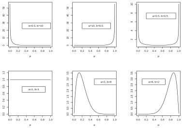
npatients have been entered in the trial. Thus the parameters of the beta prior distribution, that is a and b, may be thought of as pseudo-data elicited such that the prior belief is that if a +b patients were treated, a will be successfully treated so that the proportion of successfully treated patients is a/(a+b). This proportion is then updated when data (sn, n) are collected to give expression (2.3). Figure 2.1 shows beta densities with different parameter values. The legends give the parameter values of the beta densities. For a beta density with parameter vector (a, b) = (0.5,10), most mass is at values of p close to 0 while for a beta density with parameter vector(a, b) = (10,0.5), most mass is at values of

pclose to 1. For a beta density with parameter vector(a, b) = (0.5,0.5), probability mass is concentrated at values ofpclose to 0 and 1. Whenp is Beta(1,1), the density is flat so that this corresponds to Uniform[0,1]. When both parameters values are greater than 1, the densities have a mode between 0 and 1. For example whenpis Beta(2,8),p = 0.1is the mode. Whena >1andb > 1the mode is

a−1

a+b₋2

(19)

0.0 0.2 0.4 0.6 0.8 1.0 0 10 20 30 40 50 p a=0.5, b=10

0.0 0.2 0.4 0.6 0.8 1.0

0 10 20 30 40 50 p a=10, b=0.5

0.0 0.2 0.4 0.6 0.8 1.0

2 4 6 8 10 p a=0.5, b=0.5

0.0 0.2 0.4 0.6 0.8 1.0

0.0 0.2 0.4 0.6 0.8 1.0 1.2 p a=1, b=1

0.0 0.2 0.4 0.6 0.8 1.0

0.0 0.5 1.0 1.5 2.0 2.5 3.0 3.5 p a=2, b=8

0.0 0.2 0.4 0.6 0.8 1.0

[image:19.612.107.483.104.368.2]

0.0 0.5 1.0 1.5 2.0 2.5 3.0 3.5 p a=8, b=2

Figure 2.1: Beta densities with different parameter values. The legends give the values of the parameters.

is Beta(1,1) and prior densities with parameter value(s) less than 1 should be used with care.

In addition to the mean value of the parameter of interest, the parameter values chosen for its prior distribution should reflect the level of uncertainty (variance) associated with the parameter of interest. The variance ofpwhich is Beta(a, b) is given by

ab

(a+b)2₍_a₊_b_{+ 1)},

(20)

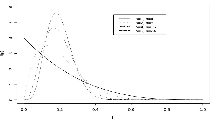
with high peaks at the mode reflecting more certainty on the true value ofp. Accordingly, Lindley and Phillips (1976) suggest referring to curves of the beta densities plotted for different values ofa andb during the elicitation process. In their paper, they give a good discussion using an example of how to elicit and quantify a beta distribution. Figure 2.2 shows curves for different values ofaandbbut with the same mean (0.2). As the values of

aandbincrease the peaks are higher and the mode moves closer to the mean 0.2. Thall and Simon (1994) refer to Lindley and Phillips (1976) for the elicitation and quantification of the beta distribution but they also introduce the idea of the width of the 90% interval (W90) running from the 5% to 95% percentiles. An investigator is asked to provide the width of an interval within which he/she is 90% confident plies. A search is then carried out to determine values ofaandbsuch that the mean ofpisa/(a+b)and the difference between the 95th quantile and the 5th quantile is equal to the specified value. The shorter the width the more informative is the prior distribution since the density curves will be more peaked.

2.2.2 Prior distribution for dose-response parameters

(21)

p

f(p)

0.0 0.2 0.4 0.6 0.8 1.0

0

1

2

3

4

5

6

[image:21.612.106.473.111.321.2]

a=1, b=4 a=2, b=8 a=4, b=16 a=6, b=24

Figure 2.2: Beta curves with same mean (0.2) but different parameter values

reviewed this form of prior distribution and some of the notation used in this section is adopted from his review.

Letp(d)denote the probability of success at dose leveld. Further suppose that given dose, successes are independent binary outcomes with probabilityp(d)and that p(d)can be modeled by a generalized linear model. Then probabilities of success are related to the dose levels through the formula

g(p(d)) =α+β f(d),

whereg(.)is a link function that links the probability of success (p(d)) to the linear pre-dictorα+β f(d), where α is the intercept parameter, β is the slope parameter and f(.)

(22)

links the probability of success to the linear predictor as follows

g(p(d)) =logit(p(d)) = log

p(d) 1₋p(d)

=α+β f(d). (2.4) Using the proposal of Bedrick et al. (1996), rather than directly elicit prior distri-butions for the parameter vector(α, β), prior distributions for the probabilities of success are elicited at some dose levels. Because the dose-response curve (2.4) is defined by two parameters (αandβ), prior distributions for probabilities of success are elicited at two dose levels. Assuming these prior distributions are independent, the joint distribution of the two probabilities of success is obtained and hence the joint distribution of the linear predictor parameters(α, β)using transformation of random variables. If there were three parameters in the linear predictor, prior distributions for probabilities of success would be elicited at three dose levels and so on. For the dose-response curve (2.4), suppose the prior distribu-tions for probabilities of success are elicited at dose levelsdi, i=−1,0. These dose levels do not have to be among the experimental dose levels. In this thesis, we will assume beta prior distributions Beta(pi;ai, bi), i = −1,0 at dose i can be elicited as described above wherepi denotes the probability of success at doseiand ai andbi may be interpreted as pseudo-data elicited as described above. Assuming the elicited beta prior distributions at the two doses are independent, then the joint prior distribution ofp(d−1)andp(d0)is given by

0

Y

i=−1

p(ai−1)

i (1−pi)(bi−1)

B(ai, bi)

.

To obtain the joint prior distribution ofαand β which we denote byπ0(α, β), the technique of transformation of random variables described in Section 2.1 is used. In equa-tion (2.1), letn = 2,X1 =p(d−1),X2 = p(d0),y1 =α, y2 = β. Assuming the logit link (2.4),

ψ1(α, β) =p(d−1) =p−1 =

exp(α+β f(d−1))

(23)

and

ψ2(α, β) =p(d0) =p0 =

exp(α+β f(d0))

1 +exp(α+β f(d0))

,

so that using equation (2.1),

π0(α, β) = 0

Y

i=−1

p(ai−1)

i (1−pi)(bi−1)

B(ai, bi) |

J|, (2.5)

wherepi, (i = −1,0)are functions of αandβ as defined above. The partial derivatives are

dψi

dα =pi(1−pi) and dψi

dβ =pi(1−pi)g(di) i=−1,0

so that

|J|=|g(d−1)−g(d0)| 0

Y

i=−1

(pi)(1−pi)

which when substituted in equation (2.5) gives

π0(α, β) = |g(d−1)−g(d0)| 0

Y

i=−1

pai

i (1−pi)bi

B(ai, bi)

.

The transformation of the dose that we are going to use in this thesis is the natural log. Hence the joint prior density ofαandβis given by,

π0(α, β) = 0

Y

i=−1

pai

i (1−pi)bi

B(ai, bi)

log

d−1

d0 . (2.6)

Suppose that a new drug is tested at k doses. Let the number of treatment successes and treatment failures at dosedi (i= 1, ..., k) be denoted byai andbi respectively. The likeli-hood function of(α, β)given the observed data is

l(α, β|x) =

k Y i=1 ni ai

pai

(24)

2.3. BAYESIAN DECISION THEORY 13

where ni = ai +bi is the number of patients allocated to dose di so that updating the distribution of (α, β) given by equation (2.6) with these data using equation (2.2), the joint posterior density forαandβis

π(α, β|x)∝

k

Y

i=−1

pai

i (1−pi)bi, (2.7) where

pi =

exp(α+β log di)

1 +exp(α+β log di)

, i=−1,0,1, ..., k.

The form of the posterior distribution given by equation (2.7) has the same form as the prior distribution given by equation (2.6) so that this prior is a conjugate prior for (α, β). Eliciting the prior distribution for (α, β) as described in this section may also have the advantage of being easier and more intuitive since it involves elicitation of the probabilities of success at several doses from investigators rather than direct elicitation of the joint probability of (α, β).

2.3 Bayesian decision theory

(25)

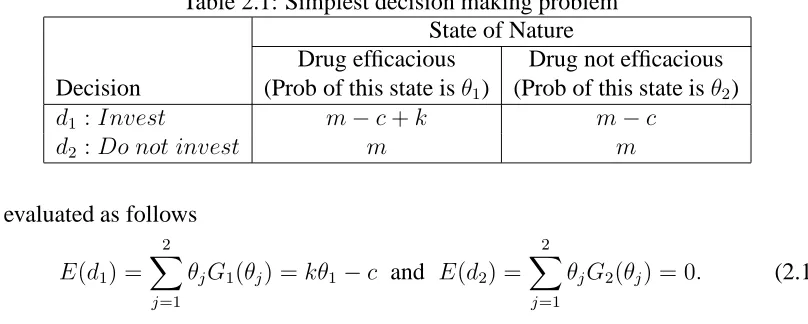
Before giving gain functions for complex decision problems, we first consider the simplest decision making problem where there are only two decisions to choose from and only two states of nature can occur. Table 2.1 summarizes this simple problem for a drug company with a capital base of£_m_{from which it can choose whether or not to invest}£_c

in a clinical trial to test efficacy of a new drug. Decision 1 is “to invest” (d1) and decision 2 is “not to invest” (d2). At the end of the clinical trial, the two states of nature are the new drug will be concluded to be efficacious (“drug is efficacious”) and the new drug will be concluded not to be efficacious (“drug is not efficacious”) with probability θ1 and θ2 respectively, whereθ1+θ2 = 1. Suppose that if the new drug is concluded to be efficacious at the end of the clinical trial, the drug company will make £_k _{from marketing the new}

drug. Then if the drug company decides to undertake the drug development, and the drug is concluded to be efficacious, the drug company will improve its capital to£₍_m₋_c₊_k₎

while if the drug is concluded not to be efficacious, then its capital will decrease by £_c

to £₍_m ₋_c₎_{. If the drug company chooses not to undertake the drug development, the}

drug company will neither lose nor gain anything regardless of whether the drug will have been concluded effective or not as shown in row corresponding to decisiond2. To compare decisiond1 andd2, the expected gain function for decisiondi (i=1,2) is defined by

E(di) = 2

X

j=1

θjGi(θj), (2.8)

whereGi(θj)is the final capital base if statej(j = 1,2)occurs for decisioni(i=1,2). The resulting expected gains from decisiond1andd2 are respectively

E(d1) = 2

X

j=1

θjG1(θj) =m+kθ1−c and E(d2) = 2

X

j=1

θjG2(θj) =m, (2.9)

(26)

[image:26.612.95.499.100.262.2]

2.3. BAYESIAN DECISION THEORY 15

Table 2.1: Simplest decision making problem State of Nature

Drug efficacious Drug not efficacious Decision (Prob of this state isθ1) (Prob of this state isθ2)

d1 :Invest m−c+k m−c

d2 :Do not invest m m

are evaluated as follows

E(d1) = 2

X

j=1

θjG1(θj) =kθ1−c and E(d2) = 2

X

j=1

θjG2(θj) = 0. (2.10)

The two expressions (2.9 and 2.10) show that the difference in expected fortune between decisionsd1 andd2only depends on the amount the drug company will make from selling the new drug if it is concluded to be effective and the amount it will lose if the new drug will be concluded not to be effective. Hence the gain functions can be compared relative to any baseline.

In the example of Table 2.1, the decision is whether to invest or not to invest. A more natural decision in clinical trials is whether to proceed from one phase of a clinical trial to the next phase. For example, in a phase II study, one may want to choose between a decision to proceed from phase II to phase III (d1) and decision to abandon drug development after the phase II study (d2). Another example would be a phase II clinical trial that allows more than one inspection of data during the trial. Before the final inspection, one may choose to stop the phase II study and proceed to phase III study (d1), stop phase II study and abandon drug development (d2) or continue with the phase II study and make another inspection (d3). Thus the number of decisions to choose from may be more than 2 but often will be finite.

Further in Table 2.1, the state of nature is that the drug is efficacious, in a clinical trial the unknown state of nature would be the probability of efficacy for an experimental drug, denoted byp_∈[0,1]. In Bayesian decision theory, the decision maker’s prior knowledge of

(27)

that are drawn from a distribution that depends on the unknown state of naturep. These data are used to update the distribution of pusing the Bayes’ theorem given by equation (2.2) resulting to a posterior distribution π(p_|x). Then the expected gain _Ga, for action

a∈ D, where_Dis the set of actions that may be chosen is given by

Z 1

0

Ga(p, n)π(p|x)dp, (2.11)

whereGa(p, n)is the gain associated with actionaand depends on the probability of suc-cesspand the number of patients in the trialn. To give an example of the form ofGa(p, n), suppose in a phase II clinical trial one of the actions that may be taken is to proceed to phase III. Suppose the average amount of money required to treat one patient in the phase II trial isk and the amount required to test a drug in a phase III trial ism ≥0. After the phase III trial, the company gets a reward denoted byl _≥ 0 which depends on the probability that the drug is concluded effective by a phase III clinical trial. This probability is given by the power function of the test denoted byκ(p). Then the gain may be expressed as

−nk−m+lκ(p),

(28)

Chapter 3 Clinical trials

In the introduction, we mentioned that in drug development, clinical trials are categorized into three phases. In this chapter, we will first in Section 3.1 give the broader definition of a clinical trial and the definition of clinical trials in the development of a new drug and then in Sections 3.2, 3.3 and 3.4 respectively, we will give the objective and review some of the statistical models used to design and analyse clinical trials in phase I, phase II and phase III. Most of the models reviewed in this chapter will assume that the clinical trials are carried out in the traditional set-up where each phase of a clinical trial is carried out separately.

3.1 What is a clinical trial?

In this section, we define a clinical trial, describe the drug development process, and de-scribe the different phases of a clinical trial. The section was compiled from various lit-erature. Some of the text books used are Wang and Bakhai (2006) and Cook and DeMets (2008). The papers reviewed in later sections were also used in developing this section. A clinical trial is a research study to test how well a new intervention such as a new therapy or

(29)

a different mode of administration of an existing drug works on people. We will consider a clinical trial in the development of a new drug. The broad aim of a clinical trial in the de-velopment of a new drug is to find out whether there is a dose (or dose range) and schedule at which the drug can be shown to be simultaneously safe and effective, to the extent that the risk-benefit relationship is acceptable. The particular subjects who may benefit from the drug, and the specific indications for its use, also need to be defined.

The modern drug development process involves a series of experiments that are carried out with specific objectives. First, tests are carried out in the laboratory in isolation from living organisms. After obtaining promising results, the next step is to test the new substance in animals (animal pharmacological studies) before the testing can proceed to human beings. The testing in human beings is what is referred to as a clinical trial and is categorized into phase I clinical trials, phase II clinical trials and phase III clinical trials.

Phase I is the stage where the drug is first tested in human beings. The primary ob-jective is to determine the safety of the new therapy. Several dose levels are made available for testing. The dose levels are determined from the animal pharmacological studies. If a safe dose (or dose range) is found, the drug is then tested for biological activity (anti-disease activity) in a small clinical trial. Such a trial is referred to as a phase II clinical trial. Before the product is released into the market, a confirmatory trial (phase III trial) has to be carried out. While phase I and II trials could include only a treatment arm, phase III trials are almost always randomized studies comparing a control (standard therapy) arm and a treatment (new drug) arm.

3.2 Phase I clinical trials

(30)

3.2. PHASE I CLINICAL TRIALS 19

to achieve this primary objective. The basic set-up of phase I clinical trials described in Section 3.2.1 is generally adopted from combining materials in the articles later cited in this section.

3.2.1 Basic set-up of a phase I clinical trial

Phase I clinical trials are typically small, having as few as 10 participants while rarely exceeding 30 participants. Except for cancer trials (oncology), where subjects are usually patients who are at an advanced stage of the disease and/or have failed to respond to the standard therapies, healthy volunteers are used. In oncology, sick patients are used because potential cancer drugs are known to be highly toxic and it would be unethical to administer them to healthy volunteers who have not been diagnosed with cancer. These are normally patients who have not responded to existing therapies. Since in oncology the subjects are patients, it may be desired that most of the patients available are allocated to the dose that will be proposed for testing in the next phases of a clinical trial. This is to enable them have maximum benefit in case the new cancer therapy has therapeutic effect on this group of patients.

Most designs, such as those proposed by O’Quigley et al. (1990), Babb et al. (1998) and Durham et al. (1997) among others, have been developed for cancer trials but can be modified for other therapies. Supposek different doses, d1 < d2 < ... < dk, are chosen for consideration in an oncology trial and we wish to establish the maximum tolerated dose (MTD). We define MTD as the dose, d∗_{, for which the probability of a medically}

unacceptable dose limiting toxicity (DLT) is equal to some specified valueθ. That is MTD is the dosed∗ _{such that}

Prob_{DLT_|d∗_}=θ.

(31)

is not necessarily the safest dose that is sought is because it is widely assumed that toxicity is a prerequisite for antidisease activity such as antitumor activity in cancer treatment. The MTDd∗_{is not necessarily one of the experimental doses}_d′

is, i= 1, ..., k. It is hoped that the lowest dose (d1) is safe and that

d1 ≤MTD≤dk.

Most investigators assume that there is an underlying dose-response relationship but not all phase I designs explicitly involve fitting the dose-response curve. Each dose level has a corresponding probability of DLT. The probability of DLT is assumed to be monotonic increasing in dose. Diagrammatical representation of the set-up is given by Figure 3.1. The experiment is performed usingk dose levelsd1, ..., dk whose respective probabilities of DLT are θ1, ..., θk. With the maximum accepted probability of DLT denoted by θ, the dose that corresponds to this value isd∗_{as is shown in the figure. In Figure 3.1, it has been}

assumed that the MTD has been captured by the experimental dose ranged1todk.

For safety reasons, the available patients (volunteers) are sequentially entered into the trial in small cohorts. Each cohort usually includes at most three volunteers. The early designs are intuitive and approach the MTD conservatively from the lowest dose (d1) while recent designs are based on statistical principles where the cohort of volunteers, for example in the Bayesian setting, are allocated to the experimental doses based on the predictive probability of toxicity at the experimental doses.

(32)

d1 ... di ... ... dk

θ1

θi

θ θk

6

d∗

dose prob. of

DLT

Figure 3.1: Phase I set-up

3.2.2 Early designs

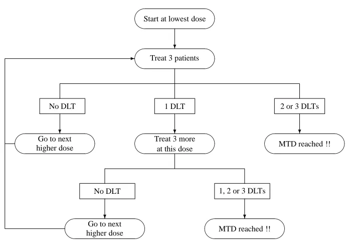
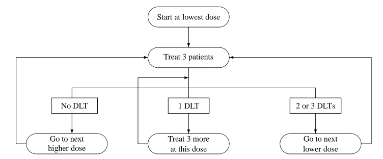
Storer (1989) describes a traditional design (which he calls design A) and also defines three more designs (B, C and D). In design A, whose flowchart is given by Figure 3.2, cohorts of 3 patients are treated at a time starting from the lowest dose. The patients’ responses are observed before allocating the next cohort to one of the experimental doses. If no DLT is observed in all 3 patients, escalation to the next higher dose occurs. If 2 or 3 DLTs are observed, the MTD is reached and the trial stops. If only 1 patient experiences a DLT, 3 more patients are allocated to the same dose and if no extra DLT is observed, escalation again continues; otherwise the MTD is reached and the trial stops.

(33)

Start at lowest dose

Treat 3 patients

?

No DLT 1 DLT 2 or 3 DLTs

Go to next higher dose

Treat 3 moreat this dose

MTD reached !! ? ? ?

No DLT 1, 2 or 3 DLTs

MTD reached !! ? ?

-Figure 3.2: Flowcharts of the traditional design (Design A)

allows de-escalation to lower doses and all available patients are entered in the trial. For this design, there is no outcome that leads to stopping so that all available patients are tested.

Storer has proposed two two-stage designs, denoted by BC and BD which combine the single-stage designs (that is B followed by either C and D). The first stage follows design B until the first toxic response occurs. From the point at which the next patient is entered at the next lower dose level, the second stage design (C or D) is implemented. He showed the two stage designs (BC and BD) estimated the MTD with reduced bias relative to the single stage designs A, C and D.

[image:33.612.121.467.78.318.2]

(34)

Start at lowest dose

Treat 3 patients

?

No DLT 1 DLT 2 or 3 DLTs

Treat 3 moreat this dose

Go to nextlower dose

?

? ?

-

-Figure 3.3: A variation of the traditional design (Design D)

3.2.3 The continual reassessment method

The Continual Reassessment Method (CRM) was developed by O’Quigley et al. (1990) for a cancer trial. Several authors, for example Babb et al. (1998), Whitehead et al. (2006), Fan and Wang (2006) and Durham et al. (1997) among others, have compared their methods’ operating characteristics with those of CRM. LetXj be a binary random variable (that is,

Xj ∈ {0,1}), where 1 denotes occurrence of a DLT and 0 nonoccurrence of a DLT for the

jth _{patient (}_j _{= 1}_{, ..., n}_{) entered in the trial. Further, as above, let}_d∗ _{(not necessarily one}

of the experimental dose levelsd1 < d2 < ... < dk) be the MTD. The probability of DLT is modeled by a simple dose-response curveψ(d, a)that depends on the dose leveld and a single parametera. The dose-response function is assumed to be monotonic indand a

and that for somea, saya0, from the setAof possible values ofa, we haveψ(d∗, a0) =θ, whereθis the maximum accepted probability of DLT.

The version of the CRM proposed by O’Quigley et al. (1990) uses the Bayesian principle where the parameterais considered to be a random variable. Let (x1, ..., xj−1), the data before experimentation on thejth_{patient, be denoted by x}

j and letπ(a|xj)denote the prior density of the parameterabefore experimentation on thejth_{patient. The form of}

[image:34.612.105.481.80.236.2]

(35)

experimentation. They take_A = (0,_∞)so that

Z ∞

0

π(a_|xj)da= 1, (j = 1, ..., n).

Using the accumulated information on the(j ₋1)patients responses, the probability of DLT at dose leveli(denoted byθij) is estimated by

θij =

Z ∞

0

ψ(di, a)π(a|xj)da, (i= 1, ..., k). (3.1)

This is the expected value of the probabilities over_A. As an approximation to equation (3.1), O’Quigley et al. (1990) suggest one could obtain the posterior mean ofaand substi-tute this in the dose-response function resulting in a simple to evaluate estimate ofθij given by

θ_ij′ =ψ(di,¯a(j)), (i= 1, ..., k), ¯a(j) =

Z ∞

0

aπ(a|xj)da.

We continue explanation of the CRM usingθ′

ij but the same procedure would be followed if one chose to useθij. In order to determine the best dose to allocate to thejth patient, the estimates of probabilities of DLTθ′

ij, (i = 1, ..., k) are compared with the accepted proportion of DLTθby defining some measure of distance∆ofθ′

ij fromθ. A commonly used choice is the absolute difference ∆(θ′

ij, θ) = |θ

′

ij −θ|. The jth entered patient is assigned to the dosedi such that∆(θ

′

ij, θ)is minimized.

Given the response of the jth _{patient, which updates the knowledge about} _a 0, the posterior distributionπ(a|xj+1) is obtained from π(a|xj) using Bayes’ formula given by equation (2.2). The likelihood of the outcome for thejth_{patient is Bernoulli given by}

φ(d(j), xj, a) = (ψ(d(j), a))xj{1−ψ(d(j), a)}1−xj,

(36)

experimenta-3.2. PHASE I CLINICAL TRIALS 25

tion withjth_{patient is}_π₍_a_|_x

j)so that the posterior distribution has density equal to

π(a|xj+1) =

φ(d(j), xj, a)π(a|xj)

R∞

0 φ(d(j), xj, u)π(u|xj)du

= π0(a)

Qj

l=1φ{d(l), xl, a}

R∞

o π0(u)

Qj

l=1φ{d(l), xl, u)}du

.

Patients are entered in this way until the results of the last patient entered are avail-able. The recommended dose level for further testing will be the dosedi (i= 1, ..., k)such that∆(θ′

i,n+1, θ)is minimized. As seen in the allocation of the patients to the dose levels, the design takes into consideration the large potential gain to the patients by aiming to treat as many patients as possible at the MTD. This makes it superior to the designs that begin testing at the lowest dose; these designs tend to under-treat more patients particularly if the MTD is the highest dose considered for experimentation.

O’Quigley and Shen (1996) proposed a likelihood based version of the CRM (CRML). Suppose(j−1)subjects have been entered in the trial and a dose-response function is de-fined as before, then the likelihood is equal to

L(a) =

j−1

Y

l=1

(ψ(dl, a))xl{1−ψ(dl, a)}1−xl,

where dl ∈ {d1, ..., dk} is the dose level allocated to patient l. To obtain an estimate fora using the maximum likelihood method, the derivative of the logarithm of the above expression is obtained which results in the score function

U(a) =

j−1

X

l=1

{xl

ψ′

ψ(dl, a)} −

j−1

X

l=1

{(1−xl)

ψ′

1−ψ(dl, a)}. (3.2)

(37)

allocated to dosedisuch that∆(ψ(di,ˆaj), θ),i= 1, ..., k, is minimized. The recommended dose level for further testing will be the dosedisuch that∆(ψ(di,ˆan+1), θ)is minimized.

Before heterogeneity, that is, when all patients experience DLTs or all patients do not experience DLTs, the equationU(a) = 0 has no solution so that it is not possible to obtain the maximum likelihood estimate of a and consequently the maximum likelihood estimateψ(di,ˆaj). Before heterogeneity in results is observed, O’Quigley and Shen (1996) suggest using the Bayesian CRM or one of the early designs described above until a DLT is observed if the first outcome is a non-DLT or vice versa. This is because the early designs do not involve estimating a parameter while allocating patients to a dose and in the Bayesian CRM, a prior distribution forais defined which is updated by the data so that we do not have problem of estimatingathrough maximum likelihood estimate. Comparison using different starting procedures show that the final results, that is the dose recommended for testing in the next phases of a clinical trial, are largely robust to the method used before heterogeneity is achieved. Operational characteristics would be expected to differ when the lower doses have a very low probability of DLT where starting with the traditional design, more patients are allocated to the lower dose levels. However, the probabilities of recommending the experimental doses for further testing are similar to starting with the Bayesian CRM. Comparison of likelihood CRM and Bayesian CRM using simulation studies indicated similar results.

(38)

to the lower doses. Despite the difference in operating characteristics with this scenario, the probabilities of recommending experimental doses for testing in the next phases of a clinical were similar in the three methods. The Bayesian CRM and CRML started with Bayesian CRM used the same prior distribution foraand the probabilities of recommend-ing the experimental doses were very close. O’Quigley and Shen (1996) observed that if less informative prior distributions were used, the results of these two methods would be closer.

3.2.4 Overdose control

An attractive idea for phase I clinical trials is to impose a safety constraint in order to minimize the chance of exposing patients to dose(s) with probability of DLT above that of the MTD. This can be achieved by requiring that a dose d cannot be administered if the predictive probability of a DLT at that dose is greater than a pre-specified value given the already collected data. Whitehead et al. (2006) propose an explicit consideration which they argue is more transparent. For example, using the Bayesian CRM, safety may be incorporated by allocating thejth _{patient to dose}_d

i such that ∆(θ

′

ij, θ)is minimized and

θ′_ij ≤θT, where ∆, θ

′

ij andθare as defined above and θT is the probability of DLT which would be considered too high to allocate patients.

(39)

MTD for binary outcomes). For thejth ₍_j _{= 1}_{, ..., n}₎_{patient, if allocation is to a dose}_d_, the probability thatdexceeds the MTD is related to the posterior CDF of the MTD and is given by the functionπj defined as

πj(d) =Prob{MTD≤d|xj},

where xj is the data at the time of jth patient, that is, the responses and the dose levels administered. Hence,πj is the conditional probability that dosedexceeds the MTD given the currently available data. Based on this criteria, thejth _{patient is allocated to the dose} leveldisuch that

πj(di) = α.

That is, each patient is allocated to a dose so that the predicted probability it exceeds the MTD is equal toα. Babb et al. (1998) assume that any dose is available within the experi-mental dose range. If only a distinct number of doses are available, thejth _{patient may be} allocated to the highest dose leveldi such that

πj(di)≤α.

3.3 Phase II clinical trials

(40)

3.3. PHASE II CLINICAL TRIALS 29

techniques have been proposed. After outlining the set-up of phase II clinical trials, we will give a review of the popular designs and the emerging new designs.

3.3.1 Set-up of phase II clinical trials

For ethical reasons, it is often important to monitor the outcomes for patients in a phase II clinical trial. For this reason, phase II trials are sometimes designed such that at least two inspections are carried out so that there are opportunities to stop early either for futility or highly promising results before all the patients available for phase II testing are entered into the trial. Suppose there arekinspections where all remaining patients are entered into the trial after the(k₋1)th_{inspection. At the}_ith_inspection₍_i_{= 1}_{, ..., k}₋₁₎_,_{three actions} (decisions) can be taken

• Action A: Stop the phase II study and abandon development of the drug

• Action P: Stop the phase II study and proceed to phase III study

(41)

fewer patients are recruited and treated. Also, reducing the development duration increases profit to the drug company because lesser time of the patent life is used to develop the new drug. On the other hand Action C is taken when the drug shows evidence of efficacy but not strong enough to suggest stopping the phase II testing after theith ₍_i _{= 1}_{, ..., k}₋₁₎ inspection to proceed to phase III testing. At thekth_{(last) inspection only actions A and P} can be taken.

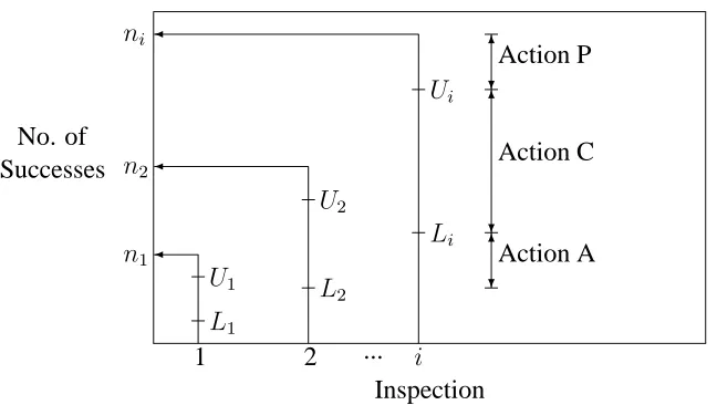
In some settings, not all three actions are considered. For example some trials allow for action P only at thekth_{inspection; that is, they do not allow for early stopping of phase} II due to highly promising results from the new drug and proceeding to phase III before all trial subjects are treated and observed. Decision (action) boundaries depend on the design being utilized. For binary data, it makes sense action P will be taken if enough successes are observed, action A will be taken if too few successes are observed and action C will be taken if the number of successes is between the number of successes required to take action A and the number of successes required to take action P. A pictorial representation of the decision boundaries is shown in Figure 3.4. In the general case, before the last inspection, if all the three actions can be taken at theith _{inspection (}_i _{= 1}_{, .., k}₋₁_{), two values} _U

i

andLi (Li < Ui)are predetermined. The two values are used as the decision boundaries for the action to be taken. Suppose at theith_{inspection the total number of treated patients} in the phase II trial isni and si are treated successfully. If si < Li, drug development is abandoned (Action A). Ifsi > Ui, phase II trial is stopped and drug development proceeds to phase III (Action P). On the other hand, ifLi ≤ si ≤ Ui, more patients are treated and

(i+ 1)th _{inspection is made (Action C). If the design does not allow Action P, no upper} valuesU′

(42)

No. of Successes

1 2 i

Inspection ...

n1

n2

ni

L1

U1 _L

2

U2

Li

Ui

6

?Action P 6

?

Action C

6

[image:42.612.116.440.81.264.2]

?Action A

Figure 3.4: A phase II setting allowing for 3 actions at each inspection

3.3.2 Frequentist designs

Frequentist designs focus on determining decision boundaries that control the error rates. Suppose that the true probabilities of success using the standard treatment and the new drug arep0 and p1 respectively. Then the new drug may be considered to be sufficiently more efficacious than the control treatment ifp1 ≥ p0 +δ, whereδ >0is a clinically relevant improvement of the new drug over the standard treatment. The hypothesis would then be to testH0 : p1 = p0 VsH1 : p1 ≥ p0 +δ. The experiment is set up such that the error of rejectingH0 when actuallyH0 is true (type I error, usually denoted byα) and the error of concludingH0 when in realityH1 is the truth (type II error, commonly denoted byβ) are controlled to some specified levels.

(43)

phase III clinical trial. Hence unlike in phase III clinical trials, Schoenfeld proposes that in a phase II clinical trial, preference should be given to minimizing type II error (hence increasing the power; power= 1₋β). He proposes setting type II error to less than 0.10 and type I error to less than 0.25.

Gehan (1961) proposed a design which has had considerable application in the past. The design has two stages. He stated that two decisions can be made

• Decision I: Drug is unlikely to be effective in a proportionp1of the patients or more

• Decision II: Drug could be effective in a proportionp1 of patients or more.

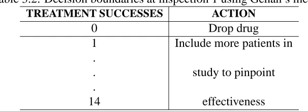
When Decision I is made at inspection 1, Action A is taken while if Decision II is made, Action C is taken. There is no opportunity for Action P. Gehan illustrated how to determine the decision boundaries by takingp1 = 0.20. Withp1 = 0.20, the chance of consecutive treatment failures is summarized in Table 3.1. The probability of treatment failure is1₋

p1 = 0.8. Assuming the observations are independent, the probability ofi(i = 1, ...,14) consecutive failures is(0.8)i_{. The chance of at least 1 success after}_i_{patients will then be} given by1−(0.8)i_{. For example as shown in the table, the chance of 3 consecutive failures} is(0.8)3 _{= 0}_.₈_×₀_.₈_×₀_._{8 = 0}_.₅₁₂_{and the chance of at least 1 success after 3 patients} have been treated will be1−(0.8)3 _{= 0}_.₄₈₈_.

(44)

[image:44.612.109.481.96.312.2]

Table 3.1: Chance of successive treatment failures when probability of success is 0.2

CONSECUTIVE CHANCE OF TREATMENT FAILURE IN GIVEN

PATIENTS CONSECUTIVE NUMBER OF PATIENTS

1 0.8

2 0.8_×0.8=0.64

3 0.8_×0.8_×0.8=0.512

. .

8 0.168

. .

11 0.086

. .

14 0.044

The number of additional subjects for the second stage is determined so that the true effectiveness of the drug is estimated with a given precision, i.e, standard error. The standard error of the estimated proportion of the treatment successes after the first sample ofn1patients is

s

p(1−p)

n1

,

wherepis the proportion of treatment successes in the first sample and n1 the size of the first sample. If the proportion of successes is approximately the same for future patients, the standard error with the total number of patients is about

s

p(1−p)

n2

, (3.3)

(45)

[image:45.612.137.440.102.212.2]

Table 3.2: Decision boundaries at inspection 1 using Gehan’s method

TREATMENT SUCCESSES ACTION

0 Drop drug

1 Include more patients in .

. study to pinpoint

.

14 effectiveness

The sample size for second stage using Gehan’s (1961) method depends on the success rate in the first stage. Also, Gehan’s design controls the error rates for the first inspection only. Simon (1989) proposed an optimal two-stage design that like Gehan’s method allows for Actions A and C but the second stage sample size does not depend on first stage success rate and his design controls the error rates for the entire phase II trial. At the first inspection, the number of successes,S1, fromn1 patients is observed. A lower boundL1 is predetermined so that ifS1 ≤ L1, action A will be taken. Otherwise action C is taken, with a further(n2 −n1)treated at the second stage. A lower boundL2 for the second stage is also set such that if the total number of successes (in both stages)S2 ≤L2, development of the drug will be abandoned.

The probability of treatment success depends on the true probability of success,

p, for the new drug. Assuming that the responses from the patients are independent and identically distributed as Bernoulli with parameterpthe probability of i (i = 0,1, ..., n1) successes in the first stage is Bin(n1, p). Thus the probability of abandoning the drug at first stage, that is prob(S1 ≤L1), is given by

L1

X

i=0

n1

i

pi(1₋p)n1−i ₌_F

B(L1;p, n1), (3.4)

(46)

Thus the probability of proceeding at stage 1 and abandoning at stage 2 is expressed as n1

X

i=L1+1

prob(S1 =iandS2−S1 ≤L2 −i;p).

Since(S2−S1)is binomial with parameter vector(n2−n1, p), with(S2−S1)independent ofS1, the above probability is

n1

X

i=L1+1

L2−i

X

j=0

n1

i

pi(1₋p)n1−i

n2 −n1

j

pj(1₋p)n2−n1−j

=

n1

X

i=L1+1

fB(i;n1, p)FB(L2−i;n2−n1, p), (3.5) wherefB denotes a binomial mass function and as before FB denotes the cumulative dis-tribution function of a binomial disdis-tribution.

The expected sample size is EN = n1 + (1 −PET)(n2 −n1)where PET is the probability of early termination after the first stage. Parametersp0,p1,αandβare specified and then the two-stage design that satisfies the error probability constraints and minimizes the expected sample size when the response probability isp0 is determined. Optimization is taken over all values ofn1and(n2−n1)as well asL1andL2. This is found by searching over the range ofL1 ∈ (0, n1)and for each value of L1 determine the maximumL2 that satisfies the type II error.

3.3.3 A Bayesian design

Thall and Simon (1994) have proposed a Bayesian design for phase II clinical trials. LetE

(47)

Let the response for the jth _{patient in the phase II clinical trial,} _X

j (j = 1,2, ...) take values 0 and 1 for treatment failure and successful treatment respectively. Assuming the responsesX′

js are independent, the total number of successes after n patients, Sn =

X1 +X2 +...+Xn, is Bin(n, pE). Suppose in an experiment after n patients, sn are treated successfully, then the posterior distributions forpE after observing data (sn, n) is denoted byπ(pE|sn, n). Assuming an improvement of sizeδis of medical significance, the objective is to determine the probability that the effect of the new treatment (pE) is greater than the effect of the standard treatment plusδ(pS+δ) expressed as

λ(sn, n;πS, πE, δ) = Prob(pS+δ < pE|Sn=snout of n)

=

Z 1−δ

pS=0

Z 1

pE=pS+δ

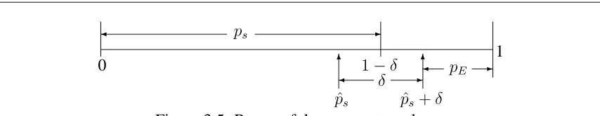
π(pE|sn, n)π0(pS)dpEdpS. (3.6) Figure 3.5 demonstrates the range of the parameter values used to obtain the probability. Since we want to determine the probability that the new drug is better than the control by effective size δ, pS and pE are integrated over values such that (pE − pS) ≥ δ. Hence parameterpsis allowed to take values from 0 to1−δ, since beyond1−δ,(pE −pS)will be less thanδ. The parameterpE is similarly integrated frompS+δto 1 to make sure that

(pE −pS)≥δ.

Thall and Simon (1994) proposed beta prior distributions for bothpE andpS. Sup-pose thatπ0(pE)is Beta(aE, bE)andπ0(ps)is Beta(aS, bS). Since there is no experimenta-tion with the control treatment, the posterior distribuexperimenta-tion ofpSis also Beta(aS, bS). For the new drug the likelihood is Binomial so that following the discussion of Section 2.2.1, the posterior distributionπ(pE|sn, n)is Beta(aE +sn, bE +n−sn)and since

Z 1

ps+δ

fβ(pE;aE+sn, bE +n−sn)dpE = 1−Fβ(pS+δ;aE +sn, bE+n−sn), wherefβ andFβ are respectively the probability density function and the cumulative dis-tribution function of a beta disdis-tribution, then equation (3.6) simplifies to

Z 1−δ

0 {

(48)

0 1−δ 1

_p_s

6 6

_δ - pE

-ˆ

[image:48.612.84.511.71.154.2]

ps pˆs+δ Figure 3.5: Range of the parameter values

wherefβ andFβ are as defined above.

Thall and Simon assume the parameters aS, bS, aE and bE can be elicited from the investigators and the parameters represent pseudo-patients. For exampleaS andbS are elicited such that if(aS+bS)patients are treated with the standard drug, thenaSwould have successful responses to the treatment whilebS will not respond positively to the standard drug. Similarly, aE patients would be treated successfully after aE +bE are treated with the new drug. Thall and Simon assume an informative prior distributionπ0(pS)and an at most slightly informative prior distributionπ0(pE). They suggest eliciting and quantifying the prior distributions by setting width of the 90% interval (W90) and examining the Beta curves as described in Section 2.2.1.

The design allows for the three actions (A, P and C) stated in Section 3.3.1. To determine the decision boundaries, a small valuepL such as (0.01-0.05) and a large value

pU such as (0.95-0.99) for equation (3.7) are predetermined. Letλ denote the expression (3.7) after the prior distributions (π0(pE), π0(pS)) and parameter values sn, nand δ are given. The lower and upper cut-offs are then given by

Un =smallest integersn such thatλ(sn, n, πS, πE,0)≥pU

Ln =Largest integersn< Unsuch that λ(sn, n, πS, πE, δ)≤pL. The decision rule afternpatients are treated is:

ifSn≤Ln, take action A, ifSn≥Un, take action P, and

(49)

wherenmaxis the maximum number of patients that can be entered into the phase II clinical trial.

3.3.4 A Bayesian decision design

The decision boundaries (rules) for the frequentist and Bayesian designs described in Sec-tions 3.3.2 and 3.3.3 respectively depend only on the number of successfully treated pa-tients. Fully Bayesian decision theory techniques can be used to define gain function which incorporate other measures such as the monetary gain for the pharmaceutical company. Stallard (1998) has proposed a method for sample size determination for phase II clinical trials using Bayesian decision theory. Here we will dwell more on Stallard’s proposal for defining decision boundaries after evaluating data rather than on sample size determina-tion. He defines a gain function that depends on the true efficacy and stage of the trial at which the decision is made. Suppose a maximum of K inspections are planned at phase II and that theith_{inspection (}_i _{= 1}_{, ..., K}_{) is carried out after a total of}_n

i patients have been entered into the trial. Further let the true probability of efficacy be denoted by p. Then the gain is a function ofpand ni and for actiona(a ∈ {A, P, C}), it is denoted by

Ga(p, ni). Actions A, P and C are as defined in Section 3.3.1. Let Xj be the indicator variable for successful treatment of patient j, j = 1, ..., ni andSni =

Pni

j=1Xj be the number of successfully treated patients afternipatients have been treated. After observing dataX1 =x1, X2 =x2, ..., Xni =xni withSni =sni, using the Bayesian decision theory principles of Section 2.3, the expected utility from actionais

Ga(sni) =E{Ga(p, ni)|sni, ni}=

Z 1

0

Ga(p, ni)π(p|sni, ni)dp,

whereπ(p_|sni, ni)is the posterior distribution of p given the data(sni, ni). The optimal action is the one with largest expected utility.

(50)

(action A) at theith _{inspection is given by}

GA(p, ni) =−nik

which is 0 (baseline value) less the number of patients entered multiplied by the cost per patient.

To proceed to phase III (action P), in addition to the cost of the phase II trial, the gain function needs to incorporate the cost of the phase III trial and the expected reward if the phase III trial shows that the new drug is efficacious. Stallard assumed that the total cost of the phase III trial is fixed and equal to some amountm(≥0). The rewardl(≥ 0)is taken to depend on the speed with which the drug can be developed. Assuming the length of phase III is fixed, the variability of speed of the drug development will depend on the length of the phase II trial and hence l will be taken to be a function of ni. Further, the reward will depend on the probability that the drug will be indicated efficacious by the phase III trial. This probability depend onpand is given by the power function of the test denoted byκ(p). The utility function for action P at theith _{inspection will thus be of the} form

GP(p, ni) =−nik−m+l(ni)κ(p).

Expectations for the two gain functions corresponding to actions A and P are given by

GA(p, ni) = E[GA(p, ni)] =−nik (3.8) and

GP(p, ni) = E[GP(p, ni)] = −nik−m+l(ni)E(κ(p)|sni, ni) (3.9) respectively, whereE(κ(p)_|sni, ni)which we define as the predictive power in Chapter 5, is the expected value ofκ(p)obtained using the posterior distribution ofpgiven(sni, ni).

Ati =K, further continuation (that is action C) is not possible. At this inspection,

(51)

C. Wheni ₆= K, the utility from action C, depends on the action that will be taken at the

(i+ 1)th_{inspection and subsequent inspections. At the}₍_i_{+ 1)}th_{inspection, if}_S

ni+1 =sni+1

and the optimal action is taken, the expected utility will be

maxa∈{A,P,C}Ga(sni+1, ni+1)

The expected utility from action C at theith _{inspection can thus be given recursively by}

GC(sni, ni) =

s_ni+ni+1−ni

X

S_ni+1=sni

maxa∈{A,P,C}{Ga(sni+1, ni+1)}fni+1(sni+1|sni, ni), (3.10)

wherefni+1(sni+1|sni, ni)is the density ofSni+1 givenSni =sni given by

fni+1(sni+1|sni, ni) =

Z 1

0

gni+1(sni+1|sni, p)π(p|sni, ni)dp

withgni+1(sni+1|sni, p)the density ofSni+1 givenSni =sni and the value ofp.

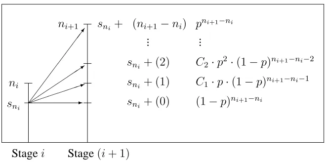
Figure 3.6 gives all possible outcomes at stage(i+ 1)and the probability of each possible outcome given the outcome at stagei. Suppose at inspectioni,sni successes are observed. With the(i+ 1)th inspection carried out afterni+1 patients have been treated, at inspection (i + 1) an extra (ni+1 −ni) patients are entered so that the extra number of successes takes values0, 1, ..., (ni+1 −ni) and consequentlySni+1 can take values

sni+ 0, sni+ 1, ..., (sni+ni+1−ni). Thus

Prob(Sni+1 =sni +s(ni+1−ni)|p) =Prob(S(ni+1−ni) =s(ni+1−ni)|p)

which is Bin((ni+1 −ni), p) where S(ni+1−ni) is the random variable denoting the extra number of successes at inspection(i+ 1). This is the distribution ofgni+1(sni+1|sni, p).

(52)

ni

sni

Stagei Stage(i+ 1)

7 1 3

-ni+1 sni + (ni+1−ni)

sni+ (2)

sni+ (1)

sni+ (0)

pni+1−ni

C2·p2·(1−p)ni+1−ni−2

C1·p·(1−p)ni+1−ni−1

[image:52.612.127.459.82.246.2]

(1−p)ni+1−ni ... ...

Figure 3.6: Possible outcomes at stage(i+ 1)

functionscanddexist that determine decision boundaries so that

maxa∈{A,P,C}Ga(sni, ni) =

            

GA(sn1, ni), sni < c(i)

GC(sni, ni), c(i)≤sni < d(i)

GP(sni, ni), d(i)≤sni.

3.3.5 Phase II studies based on therapeutic benefit and toxicity

The phase II designs described above focussed only on efficacy data. However, it may be desirable to make the decision on which doses to consider for further testing based on both efficacy and safety data. Both frequestists and Bayesian methods that use both efficacy and safety are available. We will mention several methods but we will describe in detail one frequentist method and two Bayesian methods.

A frequentist method

Dose selection in seamless phase II/III clinical trials based on efficacy and toxicity

Dose Selection in Seamless Phase II/III Clinical

Trials based on Efficacy and Toxicity

Peter Kung’u Kimani

Thesis

Doctor of Philosophy in Statistics

Department of Statistics

Contents

List of Tables

List of Figures

Acknowledgments

Declarations

Abstract

Chapter 1

Introduction

Chapter 2

Statistical background

2.1

Transformation of random variables

2.2

Review of Bayesian principle

2.2.1

Eliciting beta prior distribution for a Bernoulli parameter

2.2.2

Prior distribution for dose-response parameters

2.3

Bayesian decision theory

Chapter 3

Clinical trials

3.1

What is a clinical trial?

3.2

Phase I clinical trials

3.2.1

Basic set-up of a phase I clinical trial

3.2.2

Early designs

3.2.3

The continual reassessment method

3.2.4

Overdose control

3.3

Phase II clinical trials

3.3.1

Set-up of phase II clinical trials

3.3.2

Frequentist designs

3.3.3

A Bayesian design

3.3.4

A Bayesian decision design

3.3.5

Phase II studies based on therapeutic benefit and toxicity