A topic based sentence representation for extractive text summarization

Proceedings of the Multiling 2019 Workshop, co-located with the RANLP 2019 conference, pages 26–34 Varna, Bulgaria, September 6, 2019.

26

A topic-based sentence representation for extractive text summarization

Nikolaos Gialitsis DIT, NKUA

[email protected]

Nikiforos Pittaras DIT, NKUA IIT, NCSR-D

[email protected]

Panagiotis Stamatopoulos DIT, NKUA

[email protected]

Abstract

We examine the effect of probabilistic topic model-based word representations, on sentence-based extractive summariza-tion. We formulate the task of sentence se-lection as a binary classification problem, and we test a variety of machine learning algorithms, exploring a range of different settings for classification and modelling. A preliminary investigation via a wide ex-perimental evaluation on the MultiLing 2015 MSS dataset illustrates that topic-based representations can prove benefi-cial to the extractive summarization pro-cess, compared to a TF-IDF baseline, with Quadratic Discriminant Analysis and Gra-dient Boosting providing the best results for micro and macro F1 score, respec-tively.

1 Introduction

In recent years, advances in the field of Natural Language Processing (NLP) have revolutionized the way machines are used to interpret human-written text. With the rapid accumulation of pub-licly available documents, from newspaper articles to social media posts, machine learning methods designed to automate data analysis are urgently needed. A problem that has been relevant since the dawn of NLP is the automatic summary extraction from a large corpus of text. The development of a consistent and time-efficient method of extractive summarization can assist journalists in their day to day tasks, as well as provide better tools for infor-mation retrieval.

Summaries need to be as brief as possible but must also capture the important elements of a text. This turns out to be a challenging task for any al-gorithm to carry out, since there is a virtually

infi-nite number of documents that can exist, and each one of them can refer to a unique concept. Natu-ral language is tricky for a computer to model; the absence or presence of a single word can shift the meaning of a whole sentence or even of a whole chapter. On the other hand, some words do not add any value to a sentence, the meaning is still the same even if we ignore them. To make matters even more complex, a word can be crucial for one article but of little importance to another.

Human brains have evolved to effectively detect complex patterns in text, to focus on the most im-portant bits of a text while ignoring those that are less important. For a machine, the importance of word or a sentence is not obvious, as it needs to be programmed with a built-in way to assess it in any given context. For the purposes of summary ex-traction, an automatic summarizer needs to be able to compare words, or sentences via computational means, and announce those with the highest scores as the most relevant for a given document. The representation, aka. the method by which these similarity scores are assigned, is of critical impor-tance to any summary extraction task.

When the representation is selected, the next step is training the model, that is, feeding the sen-tences represented as numerical sequences, to a machine learning procedure. If the representation and the dataset are suitable for the goal we are try-ing to accomplish, we can expect that the model will be able to predict which words or sentences are more important to a given document. Sum-ming up all the sentences that the model considers to be important, results in a summary of the input text.

2 Related work

2.1.1 Semantic Topics.

Topics can be viewed as semantic groups that re-fer to a particular portion of reality. A document can refer to one or more distinct topics, which hu-mans can often easily distinguish. For example, the words ”fishing”, ”boat” , ”waves” , have some-thing in common; they are all affiliated with the sea. We can think of Sea as one topic, which con-tains these three words. However, topics are not always that identifiable and there can be broader or narrower topics. Resuming the previous exam-ple, alternatively, there can exist a topic on fishing , another one on boats and another one on ocean waves. Each one of them contains a number of words that are directly tied to that concept.

As demonstrated, there is no unique way to infer topics from an input document. It depends on the representation, the way that we measure the similarity scores between two words.It only makes sense that if two words are similar, they will have a high chance of belonging to the same topic.This statement derives from the distribu-tional hypothesis in linguistics which proposes that words that occur in similar contexts tend to have similar meanings (Harris, 1954) However, we have to keep in mind that one word can also belong to one or more topics and that the number of topics in a document is also not known.

2.1.2 Latent Dirichlet Allocation.

Topic models can infer topics by observing the distribution of words across documents. This can be accomplished with Latent Dirichlet Allocation (LDA) (Steyvers and Griffiths,2017;Blei,2012), a generative statistical model that makes the hy-pothesis that there exists an underlying distribu-tion of words,topics and documents, which gener-ated the input text collection. Using probabilistic topic model jargon, the words of a document are called ”observed variables”, whereas the variables of the topic structure are called ”hidden variables”. Using an iterative process, the model estimates the posterior distribution of the hidden variables given the observed variables. However, the vast amount of topic structures that can exist result in exponen-tial complexities of computation. For this reason, sampling-based algorithms have been developed , such as Gibbs sampling.

2.1.3 Gibbs sampling

In Gibbs sampling (Steyvers and Griffiths,2017), a Markov chain (i.e., a sequence of random vari-ables, each only dependent on the previous) is con-structed, using samples from the distribution of hidden variables. The assignment of words to top-ics is sampled iteratively until the Markov chain converges to the target distribution. In the be-ginning of this procedure, each word is randomly assigned to a topic and in each subsequent itera-tion, the word-topic assignments are re-evaluated, which might result in words passing through mul-tiple topics during the process.

2.2 Vector Space Models

Vector Space Model (VSM) approaches project the input to an-dimensional vector representation, where the semantic similarity of the points is de-termined by their distance (e.g cosine, euclidean, etc.) in the projected vector space. Feature vector representations are widely used in Machine Learn-ing tasks, e.g. for classification, clusterLearn-ing, etc. of a collection of input items (Turney and Pantel,

2010).

2.2.1 Bag-of-words approaches

A popular way to represent a set of documents as feature vectors has been the bag-of-words ap-proach (Salton et al.,1975), where a sentence can be represented as a vector of word features. Each vector coordinate expresses word statistics, such as frequency or the Term Frequency-Inverse Doc-ument Frequency (TF-IDF) (Jones,2004) value of a given word in the source texts. By mapping a word to its TF-IDF value, words receive a high weight when they appear often in the referenced document, but rarely in other documents of the set. The benefit of this approach is that it suppresses common words that appear in the majority of doc-uments, without containing any semantic value for the task. It has been demonstrated that the ap-proach can result in significant improvements over raw frequency approaches in a variety of informa-tion retrieval tasks. (Salton and Buckley,1988).

2.3 Extractive Summarization

formed of three relatively independent tasks : (Rao and Gudivada,2018)

1. Construction of an intermediate representa-tion of the input text based on the key aspects of the text

2. Scoring the sentences based on the selected representation

3. Selection of the summary comprising of a number of sentences

Gupta and Lehal(2010) define a different divi-sion of tasks, which includes a pre-processing and a processing step. The pre-processing step also includes: sentence boundary identification, stop-word elimination, and stemming. During the pro-cessing step, weights are assigned to specific sen-tence features by a feature-wise weighting mech-anism, with the top ranked sentences being in-cluded in the final summary. In this study, we will follow the paradigm, proposed byRao and Gudi-vada(2018).

There are two types of representation-based ap-proaches: 1) topic representations and indicator representations. A Topic representation trans-forms the text into an intermediate form and in-terprets the topic(s) discussed in the text. The techniques used for this, differ in terms of their complexity, and are divided into frequency-driven approaches, topic word approaches, latent seman-tic analysis and Bayesian topic models. Indica-tor representation describes every sentence as a list of formal features (indicators) of importance such as sentence length, position in the document, or having certain phrases; the use of indicators was demonstrated byJ et al.(2008).

2.3.1 Sentence-based summarization

In contrast to bag-of-words representations that suffer from the curse of dimensionality ( Bell-man,1958), more sophisticated recent approaches produce sentence vectors in a lower dimensional space , such as a latent-topic space. Many such these methods utilize topic clusters in order to lo-cate the centroids (or medoids in non-euclidean spaces) that best represent the sentences in the top-ics. Then the score of each sentence is assigned in respect to its distance from the clusters’ represen-tatives. For example, Thomas et al.(2015) used a graph-based procedure where each node of the graph represents a sentence and the edges’ weights reflect the similarity between the connected nodes. Next, a PageRank/TextRank algorithm is applied

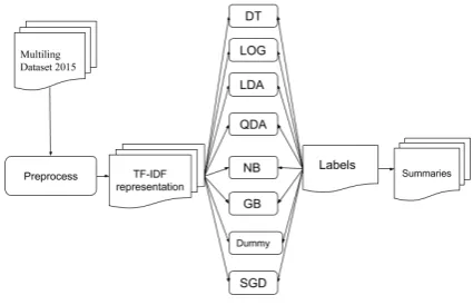
Figure 1: The pipeline for the TF-IDF-based ex-tractive summarization

to extract the sentence representatives based on the graph centrality. In another topic-based ap-proach,featured byVicente et al. (2015) Principal Component Analysis (PCA) was used to project the sentences into a lower-dimension space. The principal components are then evaluated and the sentences with the highest scores get selected to appear in the summary.

2.3.2 Contributions

There are some limitations with the majority of the existing topic-based summarization methods. First, they work directly in the sentence space and the term-topic information embedded in the sen-tences is ignored.

In this study, we combine the simplicity of word-level approaches with the power of proba-bilistic topic models; instead of limiting word in-formation to a single value (e.g. frequency or TF-IDF weight), we model sentences with word-level topic assignments. This approach is supported by a clear and rigorous probabilistic interpreta-tion (rather than some ad-hoc sentence-level ag-gregation of a multitude of unrelated scores) and produces rich, semantic sentence-level representa-tions.

3 Proposed Method

3.1 Binary classification modelling

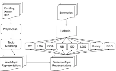
Figure 2: pipeline for topic-modeling based ex-tractive summarization

transformed to a subset ofM sentence summaries O = {oj}, oj ∈ S, j ∈ {1. . . M}via a classifier that maps each sentence to a binary label (denoted inclusion in the summary or not). The classifica-tion model should selectOsuch that the concate-nation of its sentences should produce a coherent, non-reductive and readable summary.

In this study, we tackle classification as a su-pervised learning procedure; it is necessary to have a set of ground truth sentences, that is, sen-tences that are indeed valid summaries of input documents. Such data (commonly referred to as “golden” summaries) are manually compiled by humans, who are considered the best summarizers (Genest et al.,2009); if a human reader can not dif-ferentiate between a human summarizer and an au-tomatic summarizer, that means that the extractive model is optimal. Using the input documents and ground truth data, the classification system can fa-cilitate learning using input sentence features to-wards a saliency detection model that implements sentence selection towards extractive summariza-tion. We detail this process in the next sections.

3.2 Topic-based Sentence Extraction

In our approach of extractive summarization, we utilize the topics’ information in word-level fea-ture vector representations using an LDA-based topic model with Gibbs sampling.

The intuition behind our proposed method fol-lows two statements:(1) the significance of a word is reflected by its contribution to a set of semantic topics (2) the significance of a sentence is reflected by patterns in its words-topics contributions.

For the purpose of formality we provide the

mathematical description of the proposed method. Given a finite set of semantic topics T =

{T1, T2, ...T|T|} over the documents’ space D,

a set of sentences per document SDi = {s1, s2, ..., sk}, and a set of words per sentence WS_Di = {w1, w2, ...wn}, we define the word-topics contribution function of a wordwas:

C(w) =

p(w, T1), p(w, T2), ...p(w, T|T|)

(1)

where the vector C(w) is the contribution of the word w to the topics set T and p(w, Ti) is the probability ofwbeing generated by the topic Ti ∈ T (after the topic model has inferred the posterior probability distributions), as defined by LDA’s term-topic distribution. In simpler terms, this probability is computed using:

p(w, Ti) =

N(w, Ti)

N(Ti) (2)

whereN(w, Ti)andN(Ti)are the number of oc-curences ofwinTi and the total number of word occurences inTi, respectively.

Further, normalization is applied over the con-tributions of each word vector, in order to project the values into the {0,1} interval, dividing each value by the maximum value in each vector :

Ci(w) =

Ci(w)

max(C(w))∀i∈ {1,|T|} (3)

wheremax(C(w))6= 0

After all word-topic contributions have been calculated, each sentences={w1, w2, ..., wn} is represented by the vector

C(s) = [C(w1), C(w2), ..., C(wn)], (4)

effectively transforming an input set of sentences S={s1, s2, ..sk}into the multi-dimensional vec-tor

S0 = [C(s1), C(s2), ..., C(sk)] (5)

order for the elements ofS0 in equation (5) to be-come uniform.

4 Experiments

4.1 Dataset and Preprocessing

We use the Multiling 2015 dataset for single-document summarization (Giannakopoulos et al.,

2015) 1. The dataset is constructed by the Mul-tiLing community (Conroy et al., 2015) from wikipedia pages, using articles annotated by human-curated summaries. It consists of 40 lan-guages, spanning 30 documents and summary sets – in our work, we restrict the evaluation to the En-glish language, i.e. work with the 30 EnEn-glish doc-uments provided.

We modify the dataset in order to align it with the extractive summarization setting (as the pro-vided summaries are not purely document sen-tences). First, the ground truth is modified, la-belling input source sentences with a label l ∈

0,1 (1 if the sentence should be included in the summary, else 0). This is computed by measur-ing the similarity of each source sentence with each human-authored summary for the document, in terms of common n-grams. I.e, each human-authored sentence gi is assigned to a maximally similar source sentence sj. Stopword filtering is applied prior to this process, and each source tence is assigned to at most one ground truth sen-tence.

Additionally, since the dataset used contains very unbalanced classes – the grand majority (with a ratio approximately 13 to 1) belonging to class 0, i.e. the class for sentences that should not be included in the summaries. To alleviate this, we employ an oversampling scheme. To limit the bias towards class 0 during the training phase of our model, we implemented oversampling, by repeat-ing the sentences belongrepeat-ing to class 1 a fixed num-ber of times arriving at a2 : 1negative to positive ratio, at most. This way, a classifier that always predicts dominant label (in this case 0) has sub-optimal performance.

Also, all letters were converted to lower-case in order for the model not to differentiate between words in the beginning and in the middle of sen-tences, such as ”apples” and ”Apples”. In addi-tion, stop words were also removed from the vo-cabulary to limit its size, without significant loss

1_{http://multiling.iit.demokritos.gr/} pages/view/1516/multiling-2015

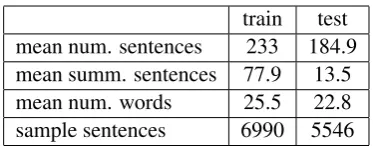
train test mean num. sentences 233 184.9 mean summ. sentences 77.9 13.5 mean num. words 25.5 22.8 sample sentences 6990 5546

Table 1: Multiling 2015 single-document summa-rization dataset characteristics.

of information.

Other preprocessing tasks such as stemming was also explored; however, they did not have a significant effect on the classification perfor-mance. After these steps, we end up with the final version of the dataset which is described in detail in table1.

4.2 Evaluation

We use the provided training and test dataset por-tion to train and evaluate the produced classifiers. The evaluation is performed in terms of micro and macro F-measure; the former is calculated by counting the total true positives, false nega-tives and false posinega-tives while the macro-averaged variant calculates metrics for each label, and finds their unweighted mean (i.e., not considering la-bel imbalance). Additionally, we compare the predicted summaries with the ground-truth as de-scribed in section 4.1, using the Rouge metric to assess performance (Lin, 2004) 2. Rouge scores reflect the overlap of n-grams between the ground-truth and the predicted summaries.

4.3 TF-IDF Sentence Classification

As a baseline model, we also implemented a IDF representation of the input dataset. The TF-IDF scores for each word-document pair are cal-culated and each sentence is represented by the vector of the tf-idf values of the words it contains. For example, a sentence withN words results in a Nw- dimensional vector, whereNw is the number of words in the sentence.

The pipeline for sentences classification using the tf-idf approach is summarized schematically in Figure 1.The scikit-learn v0.21.3 machine learn-ing library3 is used for building and training the models.

2

Metric DT KNN GB NB LDA QDA Dummy LOG SGD

macro-f1 0,497 0,511 0,514 0,514 0,527 0,080 0,452 0,527 0,481 micro-f1 0,898 0,900 0,918 0,911 0,903 0,083 0,643 0,883 0,927

Table 2: TF-IDF sentence classification results.

4.4 Topic Modeling-based Classification of sentences

For the production of the topics and the topic-vectors we used MALLET, a Java framework for various common tasks in NLP, including topic-modeling (McCallum, 2002). Using this tool, we inferred topics over the corpus of the docu-ments in the training set. We subsequently rep-resent firstly the words, and lastly the sentences, of the documents in the training set by their topic-contributions as described in section3.2. By de-fault, MALLET ignores all 1-letter and 2-letter words. Additionally, we use the NLTK english stop-words list for stop-word filtering4.

We test the trained topic model by extracting word and sentence-level probabilistic vector rep-resentations from the test set. Any word in the test set not present in the training set, is represented as a zero-vector of topic-contributions.

The pipeline for sentence classification using the topics-based approach can be visualized in fig-ure2and is outlined below:

• Infer k topics using MALLET’s topic model from the training set

• Represent each sentence in the training set using the equation (4).

• Train a classifier on the topics-represented training set

• Represent each sentence in the test set using the trained model from Step 1

• Predict the labels in the represented test set

• Evaluate the classifier using the micro and macro f-measures

5 Results and Discussion

5.1 Classification Results

The experimental results of the classification on the Multiling Dataset, evaluated with the micro-f1 and macro-micro-f1 scores are displayed in tables 2

and4, for the TF-IDF representation and the topic-based representation, respectively. Baseline re-sults using a simple rule-based classifier (Dummy)

4_{https://gist.github.com/sebleier/} 554280

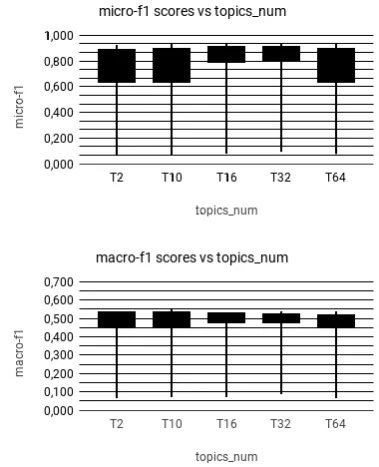
Table 3: Comparison of the micro (top) and macro (bottom) f1 performance of topic modeling, based based on the selection of the number of topics

are also reported, generating predictions with re-spect to the training set’s class distribution – it is thus not influenced by the representation. Dummy gives a micro-f1 score of 0.643 and a macro-f1 score of0.452.

For TF-IDF, the best macro-f1 score recorded is 0.527 achieved by the Linear Discriminant Analysis (LDA) and Logistic Regression Classi-fiers (LOG) and the best micro-f1 score is0.927, given by the Stochastic Gradient Descent Clas-sifier (SGD). TF-IDF achieves significantly bet-ter classification results than Dummy , improv-ing micro-f1 by 28%and macro-f1 by 7%, veri-fying the effectiveness of simple bag-of-word ap-proaches.

candi-MICRO F-MEASURE

Topics DT KNN GB NB LDA QDA Dummy LOG SGD

2 0,885 0,812 0,884 0,922 0,879 0,102 0,643 0,754 0,073 10 0,889 0,752 0,895 0,078 0,873 0,175 0,643 0,782 0,927

16 0,889 0,802 0,908 0,080 0,884 0,928 0,643 0,800 0,927 32 0,894 0,864 0,909 0,093 0,866 0,927 0,643 0,813 0,927

64 0,892 0,872 0,916 0,149 0,861 0,927 0,643 0,856 0,073 mean 0,890 0,820 0,902 0,264 0,873 0,612 0,643 0,801 0,585 std 0,003 0,044 0,011 0,330 0,008 0,387 0,000 0,034 0,418

MACRO F-MEASURE

Topics DT KNN GB NB LDA QDA Dummy LOG SGD

2 0,535 0,524 0,535 0,489 0,531 0,101 0,452 0,513 0,068 10 0,532 0,506 0,546 0,073 0,535 0,172 0,452 0,520 0,481 16 0,528 0,513 0,534 0,076 0,533 0,505 0,452 0,517 0,481 32 0,537 0,517 0,531 0,091 0,522 0,481 0,452 0,521 0,481 64 0,517 0,512 0,516 0,149 0,539 0,484 0,452 0,527 0,068

mean 0,530 0,514 0,532 0,176 0,532 0,349 0,452 0,520 0,316 std 0,007 0,006 0,010 0,159 0,006 0,175 0,000 0,005 0,202

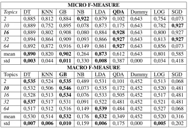
Table 4: Topic modeling results in micro and macro F1 score.

date values for the number of topics, visualized in box-plots presented in table3. By analyzing table

4and the box-plots, we concluded that a satisfac-tory number of topics is10for this particular task, as for thisk, the Gradient Boosting Classifier (GB) records the highest macro-f1 score. Our decisions are biased towards the macro-f1 instead of the micro-f1 score, since even after the over-sampling of the dataset, the classes are still heavily imbal-anced. In addition, we are mostly interested in the sentences that should be included in the summary, which belong to the smaller class. One thing to note, is that as the topic dimension increases, the macro-f1 performance of the Quadratic Discrimi-nant Analysis classifier increases rapidly between Topics 2 and Topics 32 where it reaches a plateau at macro F1≈0.48.

Topic-modeling improves on the measures of TF-IDF and Dummy, with a0.928micro-f1 score given by the Quadratic Discriminant Analysis (Topics 16) and a0.546macro-f1 score given by Gradient Boosting Classifier(Topics 10) resulting in a 3.6% increase in performance, in compari-son with the TF-IDF macro-f1 score. The worst-performing classifiers for the selected number of topics are the Naive Bayes (NB) and Quadratic Discriminant Analysis classifiers.

Finally, considering across-topics averages, SGD, QDA and NB appear to be the least stable configurations, while GB, LDA and DT are among

the top performers.

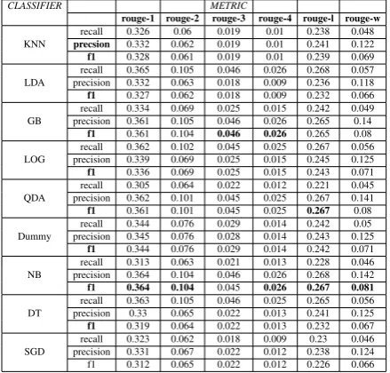
5.2 Rouge scores

The rouge scores of the summaries produced by the representation-classifier combinations are dis-played in tables5and6. Even though we observed considerable differences in the classification phase between the two representations overall, the final rouge scores are more similar than expected. Bold values correspond to the maximum f-measures for each rouge-metric.

For the TF-IDF, the highest rouge-scores across all classifiers were given by the Quadratic Dis-criminant Analysis (QDA), while for the Topics-representation, the highest values were recorded by the Naive Bayes Classifier (NB) and Gradient Boosting (GB). The TF-IDF representation results in slightly better rouge-1 to rouge-4 scores while the Topics-based representation produces better rouge-l and rouge-w scores.

6 Conclusions

us-CLASSIFIER METRIC

rouge-1 rouge-2 rouge-3 rouge-4 rouge-l rouge-w recall 0,226 0,042 0,013 0,007 0,170 0,034 KNN precision 0,307 0,056 0,017 0,008 0,232 0,127 f1 0,245 0,046 0,014 0,007 0,186 0,051 recall 0,127 0,025 0,008 0,003 0,096 0,019 LDA precision 0,161 0,036 0,017 0,011 0,120 0,065 f1 0,136 0,027 0,010 0,004 0,103 0,029 recall 0,164 0,032 0,008 0,004 0,132 0,026 GB precision 0,258 0,060 0,019 0,013 0,199 0,113 f1 0,186 0,038 0,010 0,005 0,149 0,040 recall 0,153 0,031 0,009 0,003 0,115 0,023 LOG precision 0,184 0,038 0,012 0,006 0,136 0,071 f1 0,162 0,034 0,010 0,004 0,122 0,034 recall 0,365 0,106 0,047 0,026 0,264 0,056 QDA precision 0,364 0,106 0,047 0,027 0,264 0,140 f1 0,365 0,106 0,047 0,027 0,264 0,080 recall 0,344 0,076 0,029 0,014 0,242 0,050 Dummy precision 0,345 0,076 0,028 0,014 0,243 0,125 f1 0,344 0,076 0,029 0,014 0,242 0,071 recall 0,208 0,034 0,006 0,001 0,148 0,029 NB precision 0,232 0,037 0,006 0,001 0,164 0,082 f1 0,216 0,035 0,006 0,001 0,154 0,042 recall 0,280 0,043 0,010 0,003 0,207 0,041 DT precision 0,323 0,045 0,010 0,003 0,239 0,122 f1 0,292 0,044 0,010 0,003 0,216 0,060 recall 0,000 0,000 0,000 0,000 0,000 0,000 SGD precision 0,000 0,000 0,000 0,000 0,000 0,000 f1 0,000 0,000 0,000 0,000 0,000 0,000

Table 5: TF-IDF Rouge Scores

CLASSIFIER METRIC

rouge-1 rouge-2 rouge-3 rouge-4 rouge-l rouge-w recall 0.326 0.06 0.019 0.01 0.238 0.048 KNN precsion 0.332 0.062 0.019 0.01 0.241 0.122 f1 0.328 0.061 0.019 0.01 0.239 0.069 recall 0.365 0.105 0.046 0.026 0.268 0.057 LDA precision 0.332 0.063 0.018 0.009 0.236 0.118 f1 0.327 0.062 0.018 0.009 0.232 0.066 recall 0.334 0.069 0.025 0.015 0.242 0.049 GB precision 0.361 0.105 0.046 0.026 0.265 0.14 f1 0.361 0.104 0.046 0.026 0.265 0.08 recall 0.362 0.102 0.045 0.025 0.267 0.056 LOG precision 0.339 0.069 0.025 0.015 0.245 0.125 f1 0.336 0.069 0.025 0.015 0.243 0.071 recall 0.305 0.064 0.022 0.012 0.221 0.045 QDA precision 0.362 0.101 0.045 0.025 0.267 0.141 f1 0.361 0.101 0.045 0.025 0.267 0.08 recall 0.344 0.076 0.029 0.014 0.242 0.05 Dummy precision 0.345 0.076 0.028 0.014 0.243 0.125 f1 0.344 0.076 0.029 0.014 0.242 0.071 recall 0.313 0.063 0.021 0.013 0.228 0.046 NB precision 0.364 0.104 0.046 0.026 0.268 0.142 f1 0.364 0.104 0.045 0.026 0.267 0.081 recall 0.363 0.105 0.046 0.025 0.265 0.056 DT precision 0.33 0.065 0.022 0.013 0.241 0.125 f1 0.319 0.064 0.022 0.013 0.232 0.067 recall 0.323 0.062 0.018 0.009 0.23 0.046 SGD precision 0.331 0.067 0.022 0.012 0.238 0.124 f1 0.312 0.065 0.022 0.012 0.226 0.066

Table 6: Topic modeling Rouge Scores

ing micro-f1 and macro-f1 scores. Based on the trained models, we produced summaries for the input documents and we compared them with the ground-truth using several Rouge-metrics. As a baseline, we also implemented a TF-IDF repre-sentation of sentences, which follows a traditional bag-of-words weighted approach.

Initial results of this early study show that topic-modeling can be beneficial for sentence classifica-tion, as it outperforms the TF-IDF representaclassifica-tion, as illustrated by the micro and macro f1 scores in our experiments, albeit this not being the case for the Rouge-based evaluation. We demonstrated that the topics-based approach can easily compete with the TF-IDF approach and shows promise in extractive summarization. Careful task-specific adjustments need to be made however, as the re-sults in the summary evaluation (using Rouge) appear underwhelming compared to those in the classification phase.

In the future, more sophisticated methods such as Principal Component Analysis(PCA) (Jolliffe,

2011) or Linear Semantic Analysis(LSA) ( Lan-dauer et al.,1998) can be applied on the presented framework of topics-based sentence representa-tion, in order to project the word-topic vectors into lower-dimensional spaces.

Additionally, more adaptive topic modelling ap-proaches could be applied, removing the need for pre-determined topic specification,(Steyvers and Griffiths,2017). Moreover, Neural Network clas-sification architectures can be explored, in addi-tion to the set of classifiers we already tested on the dataset. A-priori knowledge on words, phrases and sentences from external sources (e.g. knowl-edge bases such as Wordnet (A. Miller et al.,

References

A. Miller, G., Beckwith, R., Fellbaum, C., Gross, D., and J. Miller, K. (1991). Introduction to WordNet: An On-line Lexical Database*. 3.

Bellman, R. (1958). Dynamic programming and stochastic control processes. Information and Con-trol, 1(3):228 – 239.

Blei, D. M. (2012). Probabilistic topic models. Com-munications of the ACM, 55(4):77.

Conroy, J. M., Kubina, J., Rankel, P. A., and Yang, J. S. (2015).Multilingual Summarization and Evaluation Using Wikipedia Featured Articles, chapter Chapter 9, pages 281–336.

Genest, P.-E., Lapalme, G., and Yousfi-Monod, M. (2009). Hextac: the creation of a manual extractive run.

Giannakopoulos, G., Kubina, J., Conroy, J., Stein-berger, J., Favre, B., Kabadjov, M., Kruschwitz, U., and Poesio, M. (2015). MultiLing 2015: Multilingual Summarization of Single and Multi-Documents, On-line Fora, and Call-center Conver-sations. In Proceedings of the 16th Annual Meet-ing of the Special Interest Group on Discourse and Dialogue, pages 270–274, Prague, Czech Republic. Association for Computational Linguistics.

Gupta, V. and Lehal, G. S. (2010). A Survey of Text Summarization Extractive Techniques. Journal of Emerging Technologies in Web Intelligence, 2(3).

Harris, Z. S. (1954). Distributional Structure. WORD, 10(2-3):146–162.

J, J., Pingali, P., Varma, V., J, J., Pingali, P., and Varma, V. (2008). Sentence Extraction Based Single Docu-ment Summarization.

Jolliffe, I. (2011). Principal Component Analysis. In Lovric, M., editor, International Encyclopedia of Statistical Science, pages 1094–1096. Springer Berlin Heidelberg, Berlin, Heidelberg.

Jones, K. S. (2004). A statistical interpretation of term specificity and its application in retrieval. page 9.

Landauer, T. K., Foltz, P. W., and Laham, D. (1998). An introduction to latent semantic analysis. Dis-course Processes, 25(2-3):259–284.

Lin, C.-Y. (2004). ROUGE: A Package for Automatic Evaluation of Summaries. page 8.

McCallum, A. K. (2002). MALLET: A Machine Learning for Language Toolkit.

Rao, C. and Gudivada, V. (2018). Computational Analysis and Understanding of Natural Languages: Principles, Methods and Applications. Handbook of Statistics. Elsevier Science.

Salton, G. and Buckley, C. (1988). Term-weighting approaches in automatic text retrieval. Information Processing & Management, 24(5):513–523.

Salton, G., Wong, A., and Yang, C.-S. (1975). A vector space model for automatic indexing. Communica-tions of the ACM, 18(11):613–620.

Steyvers, M. and Griffiths, T. (2017). Probabilistic Topic Models. page 15.

Thomas, S., Beutenm¨uller, C., de la Puente, X., Remus, R., and Bordag, S. (2015). ExB Text Summarizer. In Proceedings of the 16th Annual Meeting of the Special Interest Group on Discourse and Dialogue, pages 260–269, Prague, Czech Republic. Associa-tion for ComputaAssocia-tional Linguistics.

Turney, P. D. and Pantel, P. (2010). From Frequency to Meaning: Vector Space Models of Semantics. Jour-nal of Artificial Intelligence Research, 37:141–188.