Online Learning of Approximate Dependency Parsing Algorithms
Ryan McDonald Fernando Pereira
Department of Computer and Information Science University of Pennsylvania
Philadelphia, PA 19104
{ryantm,pereira}@cis.upenn.edu
Abstract
In this paper we extend the maximum spanning tree (MST) dependency parsing framework of McDonald et al. (2005c) to incorporate higher-order feature rep-resentations and allow dependency struc-tures with multiple parents per word. We show that those extensions can make the MST framework computationally in-tractable, but that the intractability can be circumvented with new approximate pars-ing algorithms. We conclude with ex-periments showing that discriminative on-line learning using those approximate al-gorithms achieves the best reported pars-ing accuracy for Czech and Danish.
1 Introduction
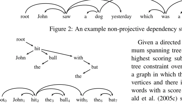
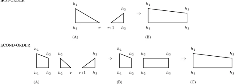
Dependency representations of sentences (Hud-son, 1984; Me´lˇcuk, 1988) model head-dependent syntactic relations as edges in a directed graph. Figure 1 displays a dependency representation for the sentence John hit the ball with the bat. This sentence is an example of a projective (or nested) tree representation, in which all edges can be drawn in the plane with none crossing. Sometimes a non-projective representations are preferred, as in the sentence in Figure 2.1 In particular, for freer-word order languages, non-projectivity is a common phenomenon since the relative positional constraints on dependents is much less rigid. The dependency structures in Figures 1 and 2 satisfy the tree constraint: they are weakly connected graphs with a unique root node, and each non-root node has a exactly one parent. Though trees are
1Examples are drawn from McDonald et al. (2005c).
more common, some formalisms allow for words to modify multiple parents (Hudson, 1984).
Recently, McDonald et al. (2005c) have shown that treating dependency parsing as the search for the highest scoring maximum spanning tree (MST) in a graph yields efficient algorithms for both projective and non-projective trees. When combined with a discriminative online learning al-gorithm and a rich feature set, these models pro-vide state-of-the-art performance across multiple languages. However, the parsing algorithms re-quire that the score of a dependency tree factors as a sum of the scores of its edges. Thisfirst-order factorizationis very restrictive since it only allows for features to be defined over single attachment decisions. Previous work has shown that condi-tioning on neighboring decisions can lead to sig-nificant improvements in accuracy (Yamada and Matsumoto, 2003; Charniak, 2000).
In this paper we extend the MST parsing frame-work to incorporate higher-order feature represen-tations of bounded-size connected subgraphs. We also present an algorithm for acyclic dependency graphs, that is, dependency graphs in which a word may depend on multiple heads. In both cases parsing is in general intractable and we provide novel approximate algorithms to make these cases tractable. We evaluate these algorithms within an online learning framework, which has been shown to be robust with respect approximate in-ference, and describe experiments displaying that these new models lead to state-of-the-art accuracy for English and the best accuracy we know of for Czech and Danish.
2 Maximum Spanning Tree Parsing
root John saw a dog yesterday which was a Yorkshire Terrier
Figure 2: An example non-projective dependency structure.
root
hit
John ball with
the bat
the
root0 John1 hit2 the3 ball4 with5 the6 bat7
Figure 1: An example dependency structure.
proposed by McDonald et al. (2005c). This formu-lation leads to efficient parsing algorithms for both projective and non-projective dependency trees with the Eisner algorithm (Eisner, 1996) and the Chu-Liu-Edmonds algorithm (Chu and Liu, 1965; Edmonds, 1967) respectively. The formulation works by defining the score of a dependency tree to be the sum of edge scores,
s(x,y) =
X
(i,j)∈y
s(i, j)
where x = x1· · ·xn is an input sentence and y
a dependency tree forx. We can viewy as a set
of tree edges and write (i, j) ∈ y to indicate an
edge inyfrom wordxito wordxj. Consider the example from Figure 1, where the subscripts index the nodes of the tree. The score of this tree would then be,
s(0,2) +s(2,1) +s(2,4) +s(2,5) +s(4,3) +s(5,7) +s(7,6)
We call this first-order dependency parsing since scores are restricted to a single edge in the depen-dency tree. The score of an edge is in turn com-puted as the inner product of a high-dimensional feature representation of the edge with a corre-sponding weight vector,
s(i, j) =w·f(i, j)
This is a standard linear classifier in which the weight vector ware the parameters to be learned during training. We should note thatf(i, j)can be based on arbitrary features of the edge and the in-put sequencex.
Given a directed graph G = (V, E), the maxi-mum spanning tree (MST) problem is to find the highest scoring subgraph of G that satisfies the tree constraint over the vertices V. By defining a graph in which the words in a sentence are the vertices and there is a directed edge between all words with a score as calculated above, McDon-ald et al. (2005c) showed that dependency pars-ing is equivalent to findpars-ing the MST in this graph. Furthermore, it was shown that this formulation can lead to state-of-the-art results when combined with discriminative learning algorithms.
Although the MST formulation applies to any directed graph, our feature representations and one of the parsing algorithms (Eisner’s) rely on a linear ordering of the vertices, namely the order of the words in the sentence.
2.1 Second-Order MST Parsing
Restricting scores to a single edge in a depen-dency tree gives a very impoverished view of de-pendency parsing. Yamada and Matsumoto (2003) showed that keeping a small amount of parsing history was crucial to improving parsing perfor-mance for their locally-trained shift-reduce SVM parser. It is reasonable to assume that other pars-ing models might benefit from features over previ-ous decisions.
Here we will focus on methods for parsing
second-order spanning trees. These models fac-tor the score of the tree into the sum of adjacent edge pair scores. To quantify this, consider again the example from Figure 1. In the second-order spanning tree model, the score would be,
s(0,−,2) +s(2,−,1) +s(2,−,4) +s(2,4,5) +s(4,−,3) +s(5,−,7) +s(7,−,6)
Here we use the second-order score function
there is no s(2,1,4) for the adjacent edges from
hittoJohnandball). This independence between left and right descendants allow us to use aO(n3) second-order projective parsing algorithm, as we will see later. We write s(xi,−, xj) when xj is the first left or first right dependent of word xi. For example, s(2,−,4) is the score of creating a dependency fromhittoball, sinceballis the first child to the right ofhit. More formally, if the word
xi0 has the children shown in this picture,
xi0
xi1 . . . xij xij+1 . . . xim
the score factors as follows:
Pj−1
k=1s(i0, ik+1, ik) +s(i0,−, ij) +s(i0,−, ij+1) +Pmk=−j1+1s(i0, ik, ik+1)
This second-order factorization subsumes the first-order factorization, since the score function could just ignore the middle argument to simulate first-order scoring. The score of a tree for second-order parsing is now
s(x,y) =
X
(i,k,j)∈y
s(i, k, j)
wherekandjare adjacent, same-side children of
iin the treey.
The second-order model allows us to condition on the most recent parsing decision, that is, the last dependent picked up by a particular word, which is analogous to the the Markov conditioning of in the Charniak parser (Charniak, 2000).
2.2 Exact Projective Parsing
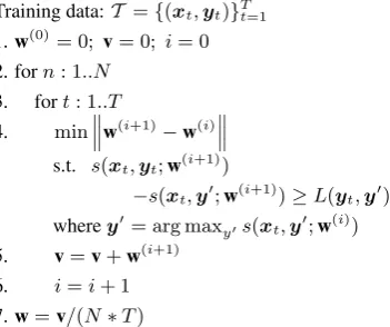
For projective MST parsing, the first-order algo-rithm can be extended to the second-order case, as was noted by Eisner (1996). The intuition behind the algorithm is shown graphically in Figure 3, which displays both the first-order and second-order algorithms. In the first-second-order algorithm, a word will gather its left and right dependents in-dependently by gathering each half of the subtree rooted by its dependent in separate stages. By splitting up chart items into left and right com-ponents, the Eisner algorithm only requires 3 in-dices to be maintained at each step, as discussed in detail elsewhere (Eisner, 1996; McDonald et al., 2005b). For the second-order algorithm, the key insight is to delay the scoring of edges until pairs
2-order-non-proj-approx(x, s)
Sentencex=x0. . . xn,x0=root
Weight functions: (i, k, j)→R
1. Lety=2-order-proj(x, s)
2. while true
3. m=−∞, c=−1, p=−1 4. forj: 1· · ·n
5. fori: 0· · ·n 6. y0=y[i→j]
7. if¬tree(y0)or∃k: (i, k, j)∈ycontinue
8. δ=s(x,y0)−s(x,y)
9. ifδ > m
10. m=δ, c=j, p=i 11. end for
12. end for 13. ifm >0 14. y=y[p→c]
15. elsereturny
16. end while
Figure 4: Approximate second-order non-projective parsing algorithm.
of dependents have been gathered. This allows for the collection of pairs of adjacent dependents in a single stage, which allows for the incorporation of second-order scores, while maintaining cubic-time parsing.
The Eisner algorithm can be extended to an arbitrary mth-order model with a complexity of
O(nm+1), form > 1. Anmth-order parsing gorithm will work similarly to the second-order al-gorithm, except that we collectmpairs of adjacent dependents in succession before attaching them to their parent.
2.3 Approximate Non-projective Parsing
Unfortunately, second-order non-projective MST parsing is NP-hard, as shown in appendix A. To circumvent this, we designed an approximate al-gorithm based on the exact O(n3) second-order projective Eisner algorithm. The approximation works by first finding the highest scoring projec-tive parse. It then rearranges edges in the tree, one at a time, as long as such rearrangements in-crease the overall score and do not violate the tree constraint. We can easily motivate this approxi-mation by observing that even in non-projective languages like Czech and Danish, most trees are primarily projective with just a few non-projective edges (Nivre and Nilsson, 2005). Thus, by start-ing with the highest scorstart-ing projective tree, we are typically only a small number of transformations away from the highest scoring non-projective tree. The algorithm is shown in Figure 4. The ex-pressiony[i → j]denotes the dependency graph
FIRST-ORDER
h1
h3 ⇒
h1 r r+1 h3
(A)
h1
h3
h1 h3
(B)
SECOND-ORDER
h1
h2 h2 h3 ⇒
h1 h2 h2 r r+1 h3
(A)
h1
h2 h2 h3 ⇒
h1 h2 h2 h3
(B)
h1
h3
h1 h3
[image:4.595.75.473.65.206.2](C)
Figure 3: AO(n3)extension of the Eisner algorithm to second-order dependency parsing. This figure shows howh1 creates a dependency to h3 with the second-order knowledge that the last dependent of
h1 wash2. This is done through the creation of asiblingitem in part (B). In the first-order model, the dependency toh3 is created after the algorithm has forgotten thath2 was the last dependent.
of what it was iny. The testtree(y)is true iff the
dependency graphysatisfies the tree constraint.
In more detail, line 1 of the algorithm setsyto
the highest scoring second-order projective tree. The loop of lines 2–16 exits only when no fur-ther score improvement is possible. Each iteration seeks the single highest-scoring parent change to
ythat does not break the tree constraint. To that
effect, the nested loops starting in lines 4 and 5 enumerate all(i, j)pairs. Line 6 setsy0to the
de-pendency graph obtained fromyby changingxj’s
parent toxi. Line 7 checks that the move fromy
toy0is valid by testing thatxj’s parent was not al-readyxiand thaty0is a tree. Line 8 computes the
score change fromytoy0. If this change is larger
than the previous best change, we record how this new tree was created (lines 9-10). After consid-ering all possible valid edge changes to the tree, the algorithm checks to see that the best new tree does have a higher score. If that is the case, we change the tree permanently and re-enter the loop. Otherwise we exit since there are no single edge switches that can improve the score.
This algorithm allows for the introduction of non-projective edges because we do not restrict any of the edge changes except to maintain the tree property. In fact, if any edge change is ever made, the resulting tree is guaranteed to be non-projective, otherwise there would have been a higher scoring projective tree that would have al-ready been found by the exact projective parsing algorithm. It is not difficult to find examples for which this approximation will terminate without returning the highest-scoring non-projective parse.
It is clear that this approximation will always
terminate — there are only a finite number of de-pendency trees for any given sentence and each it-eration of the loop requires an increase in score to continue. However, the loop could potentially take exponential time, so we will bound the num-ber of edge transformations to a fixed value M. It is easy to argue that this will not hurt perfor-mance. Even in freer-word order languages such as Czech, almost all non-projective dependency trees are primarily projective, modulo a few non-projective edges. Thus, if our inference algorithm starts with the highest scoring projective parse, the best non-projective parse only differs by a small number of edge transformations. Furthermore, it is easy to show that each iteration of the loop takes
O(n2)time, resulting in aO(n3+M n2)runtime algorithm. In practice, the approximation termi-nates after a small number of transformations and we do not need to bound the number of iterations in our experiments.
We should note that this is one of many possible approximations we could have made. Another rea-sonable approach would be to first find the highest scoringfirst-order non-projective parse, and then re-arrange edges based on second order scores in a similar manner to the algorithm we described. We implemented this method and found that the results were slightly worse.
3 Danish: Parsing Secondary Parents
root Han spejder efter og ser elefanterne
He looks for and sees elephants
Figure 5: An example dependency tree from the Danish Dependency Treebank (from Kromann (2003)).
word to have multiple parents. Examples include verb coordination in which the subject or object is an argument of several verbs, and relative clauses in which words must satisfy dependencies both in-side and outin-side the clause. An example is shown in Figure 5 for the sentenceHe looks for and sees elephants. Here, the pronounHeis the subject for both verbs in the sentence, and the nounelephants
the corresponding object. In the Danish Depen-dency Treebank, roughly5%of words have more than one parent, which breaks the single parent (or tree) constraint we have previously required on dependency structures. Kromann also allows for cyclic dependencies, though we deal only with acyclic dependency graphs here. Though less common than trees, dependency graphs involving multiple parents are well established in the litera-ture (Hudson, 1984). Unfortunately, the problem of finding the dependency structure with highest score in this setting is intractable (Chickering et al., 1994).
To create an approximate parsing algorithm for dependency structures with multiple parents, we start with our approximate second-order non-projective algorithm outlined in Figure 4. We use the non-projective algorithm since the Danish De-pendency Treebank contains a small number of non-projective arcs. We then modify lines 7-10 of this algorithm so that it looks for the change in parentor the addition of a new parent that causes the highest change in overall score and does not create a cycle2. Like before, we make one change per iteration and that change will depend on the resulting score of the new tree. Using this sim-ple new approximate parsing algorithm, we train a new parser that can produce multiple parents.
4 Online Learning and Approximate
Inference
In this section, we review the work of McDonald et al. (2005b) for online large-margin dependency
2We are not concerned with violating the tree constraint.
parsing. As usual for supervised learning, we as-sume a training set T = {(xt,yt)}Tt=1,
consist-ing of pairs of a sentencextand its correct depen-dency representationyt.
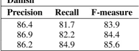
The algorithm is an extension of the Margin In-fused Relaxed Algorithm (MIRA) (Crammer and Singer, 2003) to learning with structured outputs, in the present case dependency structures. Fig-ure 6 gives pseudo-code for the algorithm. An on-line learning algorithm considers a single training instance for each update to the weight vector w. We use the common method of setting the final weight vector as the average of the weight vec-tors after each iteration (Collins, 2002), which has been shown to alleviate overfitting.
On each iteration, the algorithm considers a single training instance. We parse this instance to obtain a predicted dependency graph, and find the smallest-norm update to the weight vector w
that ensures that the training graph outscores the predicted graph by a margin proportional to the loss of the predicted graph relative to the training graph, which is the number of words with incor-rect parents in the predicted tree (McDonald et al., 2005b). Note that we only impose margin con-straints between the single highest-scoring graph and the correct graph relative to the current weight setting. Past work on tree-structured outputs has used constraints for the k-best scoring tree (Mc-Donald et al., 2005b) or even all possible trees by using factored representations (Taskar et al., 2004; McDonald et al., 2005c). However, we have found that a single margin constraint per example leads to much faster training with a negligible degrada-tion in performance. Furthermore, this formula-tion relates learning directly to inference, which is important, since we want the model to set weights relative to the errors made by an approximate in-ference algorithm. This algorithm can thus be viewed as a large-margin version of the perceptron algorithm for structured outputs Collins (2002).
Training data:T ={(xt,yt)}Tt=1
1.w(0)= 0; v= 0; i= 0 2. forn: 1..N
3. fort: 1..T 4. min‚‚
‚w
(i+1)−w(i)‚‚ ‚
s.t. s(xt,yt;w(i+1))
−s(xt,y0;w(i+1))≥L(yt,y0)
wherey0= arg maxy0s(xt,y0;w(i))
5. v=v+w(i+1)
[image:6.595.328.511.62.108.2]6. i=i+ 1 7.w=v/(N∗T)
Figure 6: MIRA learning algorithm. We write
s(x,y;w(i)) to mean the score of tree y using
weight vectorw(i).
approximate inference and adjusts weights to cor-rect for them. The work of Daum´e and Marcu (2005) formalizes this intuition by presenting an online learning framework in which parameter up-dates are made directly with respect to errors in the inference algorithm. We show in the next section that this robustness extends to approximate depen-dency parsing.
5 Experiments
The score of adjacent edges relies on the defini-tion of a feature representadefini-tionf(i, k, j). As noted earlier, this representation subsumes the first-order representation of McDonald et al. (2005b), so we can incorporate all of their features as well as the new second-order features we now describe. The old first-order features are built from the parent and child words, their POS tags, and the POS tags of surrounding words and those of words between the child and the parent, as well as the direction and distance from the parent to the child. The second-order features are built from the following conjunctions of word and POS identity predicates
xi-pos,xk-pos,xj-pos
xk-pos,xj-pos
xk-word,xj-word
xk-word,xj-pos
xk-pos,xj-word
wherexi-pos is the part-of-speech of theithword in the sentence. We also include conjunctions be-tween these features and the direction and distance from siblingjto siblingk. We determined the use-fulness of these features on the development set, which also helped us find out that features such as the POS tags of words between the two siblings would not improve accuracy. We also ignored
fea-English
Accuracy Complete
1st-order-projective 90.7 36.7 2nd-order-projective 91.5 42.1
Table 1: Dependency parsing results for English.
Czech
Accuracy Complete
[image:6.595.75.251.63.210.2]1st-order-projective 83.0 30.6 2nd-order-projective 84.2 33.1 1st-order-non-projective 84.1 32.2 2nd-order-non-projective 85.2 35.9
Table 2: Dependency parsing results for Czech.
tures over triples of words since this would ex-plode the size of the feature space.
We evaluate dependencies on per word accu-racy, which is the percentage of words in the sen-tence with the correct parent in the tree, and on complete dependency analysis. In our evaluation we exclude punctuation for English and include it for Czech and Danish, which is the standard.
5.1 English Results
To create data sets for English, we used the Ya-mada and Matsumoto (2003) head rules to ex-tract dependency trees from the WSJ, setting sec-tions 2-21 as training, section 22 for development and section 23 for evaluation. The models rely on part-of-speech tags as input and we used the Ratnaparkhi (1996) tagger to provide these for the development and evaluation set. These data sets are exclusively projective so we only com-pare the projective parsers using the exact projec-tive parsing algorithms. The purpose of these ex-periments is to gauge the overall benefit from in-cluding second-order features with exact parsing algorithms, which can be attained in the projective setting. Results are shown in Table 1. We can see that there is clearly an advantage in introducing second-order features. In particular, the complete tree metric is improved considerably.
5.2 Czech Results
[image:6.595.134.229.600.654.2]ac-Danish
Precision Recall F-measure
[image:7.595.318.455.67.118.2]2nd-order-projective 86.4 81.7 83.9 2nd-order-non-projective 86.9 82.2 84.4 2nd-order-non-projective w/ multiple parents 86.2 84.9 85.6
Table 3: Dependency parsing results for Danish.
tually non-projective. Results are shown in Ta-ble 2. McDonald et al. (2005c) showed a substan-tial improvement in accuracy by modeling non-projective edges in Czech, shown by the difference between two first-order models. Table 2 shows that a second-order model provides a compara-ble accuracy boost, even using an approximate projective algorithm. The second-order non-projective model accuracy of85.2%is the highest reported accuracy for a single parser for these data. Similar results were obtained by Hall and N ´ov´ak (2005) (85.1% accuracy) who take the best out-put of the Charniak parser extended to Czech and rerank slight variations on this output that intro-duce non-projective edges. However, this system relies on a much slower phrase-structure parser as its base model as well as an auxiliary rerank-ing module. Indeed, our second-order projective parser analyzes the test set in 16m32s, and the non-projective approximate parser needs 17m03s to parse the entire evaluation set, showing that run-time for the approximation is completely domi-nated by the initial call to the second-order pro-jective algorithm and that the post-process edge transformation loop typically only iterates a few times per sentence.
5.3 Danish Results
For our experiments we used the Danish Depen-dency Treebank v1.0. The treebank contains a small number of inter-sentence and cyclic depen-dencies and we removed all sentences that tained such structures. The resulting data set con-tained 5384 sentences. We partitioned the data into contiguous 80/20 training/testing splits. We held out a subset of the training data for develop-ment purposes.
We compared three systems, the standard second-order projective and non-projective pars-ing models, as well as our modified second-order non-projective model that allows for the introduc-tion of multiple parents (Secintroduc-tion 3). All systems use gold-standard part-of-speech since no trained tagger is readily available for Danish. Results are shown in Figure 3. As might be expected, the
non-projective parser does slightly better than the pro-jective parser because around 1% of the edges are non-projective. Since each word may have an ar-bitrary number of parents, we must use precision and recall rather than accuracy to measure perfor-mance. This also means that the correct training loss is no longer the Hamming loss. Instead, we use false positives plus false negatives over edge decisions, which balances precision and recall as our ultimate performance metric.
As expected, for the basic projective and non-projective parsers, recall is roughly 5% lower than precision since these models can only pick up at most one parent per word. For the parser that can introduce multiple parents, we see an increase in recall of nearly 3% absolute with a slight drop in precision. These results are very promising and further show the robustness of discriminative on-line learning with approximate parsing algorithms.
6 Discussion
We described approximate dependency parsing al-gorithms that support higher-order features and multiple parents. We showed that these approxi-mations can be combined with online learning to achieve fast parsing with competitive parsing ac-curacy. These results show that the gain from al-lowing richer representations outweighs the loss from approximate parsing and further shows the robustness of online learning algorithms with ap-proximate inference.
those in our current second-order model.
Acknowledgments
This work was supported by NSF ITR grants 0205448.
References
E. Charniak. 2000. A maximum-entropy-inspired parser. InProc. NAACL.
D.M. Chickering, D. Geiger, and D. Heckerman. 1994. Learning bayesian networks: The combination of knowledge and statistical data. Technical Report MSR-TR-94-09, Microsoft Research.
Y.J. Chu and T.H. Liu. 1965. On the shortest arbores-cence of a directed graph.Science Sinica, 14:1396– 1400.
M. Collins and B. Roark. 2004. Incremental parsing with the perceptron algorithm. InProc. ACL.
M. Collins, J. Hajiˇc, L. Ramshaw, and C. Tillmann. 1999. A statistical parser for Czech. InProc. ACL.
M. Collins. 2002. Discriminative training methods for hidden Markov models: Theory and experiments with perceptron algorithms. InProc. EMNLP.
K. Crammer and Y. Singer. 2003. Ultraconservative online algorithms for multiclass problems.JMLR.
H. Daum´e and D. Marcu. 2005. Learning as search op-timization: Approximate large margin methods for structured prediction. InProc. ICML.
J. Edmonds. 1967. Optimum branchings. Journal of Research of the National Bureau of Standards, 71B:233–240.
J. Eisner. 1996. Three new probabilistic models for dependency parsing: An exploration. InProc. COL-ING.
J. Hajiˇc, E. Hajicova, P. Pajas, J. Panevova, P. Sgall, and B. Vidova Hladka. 2001. The Prague Dependency Treebank 1.0 CDROM. Linguistics Data Consor-tium Cat. No. LDC2001T10.
K. Hall and V. N´ov´ak. 2005. Corrective modeling for non-projective dependency parsing. InProc. IWPT.
R. Hudson. 1984.Word Grammar. Blackwell.
M. T. Kromann. 2001. Optimaility parsing and local cost functions in discontinuous grammars. InProc. FG-MOL.
M. T. Kromann. 2003. The danish dependency tree-bank and the dtag treetree-bank tool. InProc. TLT.
R. McDonald, K. Crammer, and F. Pereira. 2005a. Flexible text segmentation with structured multil-abel classifi cation. InProc. HLT-EMNLP.
R. McDonald, K. Crammer, and F. Pereira. 2005b. On-line large-margin training of dependency parsers. In
Proc. ACL.
R. McDonald, F. Pereira, K. Ribarov, and J. Hajiˇc. 2005c. Non-projective dependency parsing using spanning tree algorithms. InProc. HLT-EMNLP.
I.A. Me´lˇcuk. 1988. Dependency Syntax: Theory and Practice. State University of New York Press.
R. Moore. 2005. A discriminative framework for bilin-gual word alignment. InProc. HLT-EMNLP.
J. Nivre and J. Nilsson. 2005. Pseudo-projective de-pendency parsing. InProc. ACL.
A. Ratnaparkhi. 1996. A maximum entropy model for part-of-speech tagging. InProc. EMNLP.
B. Taskar, D. Klein, M. Collins, D. Koller, and C. Man-ning. 2004. Max-margin parsing. InProc. EMNLP.
H. Yamada and Y. Matsumoto. 2003. Statistical de-pendency analysis with support vector machines. In
Proc. IWPT.
A 2nd-Order Non-projective MST
Parsing is NP-hard
Proof by a reduction from 3-D matching (3DM).
3DM: Disjoint setsX, Y, Zeach withmdistinct elements and a setT ⊆X×Y×Z. Question: is there a subsetS⊆T such that|S|=mand eachv∈X∪Y∪Zoccurs in exactly one element ofS.
Reduction: Given an instance of 3DM we defi ne a graph in which the vertices are the elements fromX∪Y ∪Z as well as an artifi cialrootnode. We insert edges fromrootto allxi ∈X as well as edges from allxi ∈X to allyi ∈Y
andzi ∈ Z. We order the words s.t. the root is on the left
followed by all elements ofX, thenY, and fi nallyZ. We then defi ne the second-order score function as follows,
s(root, xi, xj) = 0, ∀xi, xj∈X
s(xi,−, yj) = 0, ∀xi∈X, yj∈Y
s(xi, yj, zk) = 1, ∀(xi, yj, zk)∈T
All other scores are defi ned to be−∞, including for edges pairs that were not defi ned in the original graph.
Theorem: There is a 3D matching iff the second-order
MST has a score ofm. Proof: First we observe that no tree
can have a score greater thanmsince that would require more thanmpairs of edges of the form(xi, yj, zk). This can only
happen when somexihas multipleyj ∈Y children or
mul-tiplezk ∈ Zchildren. But if this were true then we would
introduce a−∞scored edge pair (e.g.s(xi, yj, y0j)). Now, if
the highest scoring second-order MST has a score ofm, that means that everyximust have found a unique pair of
chil-drenyjandzkwhich represents the 3D matching, since there
would bemsuch triples. Furthermore,yjandzkcould not
match with any otherx0
isince they can only have one
incom-ing edge in the tree. On the other hand, if there is a 3DM, then there must be a tree of weightmconsisting of second-order edges(xi, yj, zk)for each element of the matchingS. Since