Twitter Geolocation using Knowledge Based Methods

7

Twitter Geolocation using Knowledge-Based Methods

Taro Miyazaki†‡ Afshin Rahimi† Trevor Cohn† Timothy Baldwin†

†The University of Melbourne

‡NHK Science and Technology Research Laboratories [email protected]

{rahimia,trevor.cohn,tbaldwin}@unimelb.edu.au

Abstract

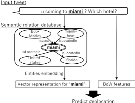
Automatic geolocation of microblog posts from their text content is particularly diffi-cult because many location-indicative terms are rare terms, notably entity names such as locations, people or local organisations. Their low frequency means that key terms observed in testing are often unseen in training, such that standard classifiers are unable to learn weights for them. We propose a method for reasoning over such terms using a knowl-edge base, through exploiting their relations with other entities. Our technique uses a graph embedding over the knowledge base, which we couple with a text representation to learn a geolocation classifier, trained end-to-end. We show that our method improves over purely text-based methods, which we ascribe to more robust treatment of low-count and out-of-vocabulary entities.

1 Introduction

Twitter has been used in diverse applications such as disaster monitoring (Ashktorab et al., 2014;

Mizuno et al., 2016), news material gathering (Vosecky et al.,2013; Hayashi et al., 2015), and stock market prediction (Mittal and Goel,2012;Si et al.,2013). In many of these applications, geolo-cation information plays an important role. How-ever, less than 1% of Twitter users enable GPS-based geotagging, so third-party service providers require methods to automatically predict geoloca-tion from text, profile and network informageoloca-tion. This has motivated many studies on estimating ge-olocation using Twitter data (Han et al.,2014).

Approaches to Twitter geolocation can be clas-sified into text-based and network-based meth-ods. Text-based methods are based on the text content of tweets (possibly in addition to textual user metadata), while network-based methods use relations between users, such as user mentions,

u coming to miami? Which hotel?

Semantic relation database

miami

miami-heat

Bob-Marley

United-states

isLocatedIn

isLocatedIn DiedIn

florida

isLocatedIn Input tweet

Entities embedding

Vector representation for “miami” BoW features

Predict geolocation

Figure 1: Basic idea of our method.

follower–followee links, or retweets. In this pa-per, we propose a text-based geolocation method which takes a set of tweets from a given user as input, performs named entity linking relative to a static knowledge base (“KB”), and jointly embeds the text of the tweets with concepts linked from the tweets, to use as the basis for classifying the location of the user. Figure1presents an overview of our method. The hypothesis underlying this re-search is that KBs contain valuable geolocation in-formation, and that this can complement pure text-based methods. While others have observed that KBs have utility for geolocation tasks (Brunsting et al., 2016; Salehi et al., 2017), this is the first attempt to combine a large-scale KB with a text-based method for user geolocation.

KB, including the large number of NEs that are unattested in the training data. This is the pri-mary advantage of our method over generating text embeddings for the named entity (“NE”) to-kens, which would only be applicable to NEs at-tested in the training data.

Our contributions are as follows: (1) we pro-pose a joint knowledge-based neural network model for Twitter user geolocation, that outper-forms conventional text-based user geolocation; and (2) we show that our method works well even if the accuracy of the NE recognition is low — a common situation with Twitter, because many posts are written colloquially, without capitaliza-tion for proper names, and with non-standard syn-tax (Baldwin et al.,2013,2015).

2 Related Work

2.1 Text-based methods

Text-based geolocation methods use text features to estimate geolocation. Unsupervised topic mod-eling approaches (Eisenstein et al., 2010; Hong et al.,2012;Ahmed et al.,2013) are one success-ful approach in text-based geolocation estimation, although they tend not to scale to larger data sets. It is also possible to use semi-supervised learning over gazetteers (Lieberman et al.,2010;Quercini et al.,2010), whereby gazetted terms are identified and used to construct a distribution over possible locations, and clustering or similar methods are then used to disambiguate over this distribution. More recent data-driven approaches extend this idea to automatically learn a gazetteer-like dictio-nary based on semi-supervised sparse-coding (Cha et al.,2015).

Supervised approaches tend to be based on bag-of-words modelling of the text, in combination with a machine learning method such as hierarchi-cal logistic regression (Wing and Baldridge,2014) or a neural network with denoising autoencoder (Liu and Inkpen, 2015). Han et al. (2012) fo-cused on explicitly identifying “location indicative words” using multinomial naive Bayes and logis-tic regression classifiers combined with feature se-lection methods, whileRahimi et al.(2015b) ex-tended this work using multi-level regularisation and a multi-layer perceptron architecture (Rahimi et al.,2017b).

2.2 Network-based methods

Twitter, as a social media platform, supports a number of different modalities for interacting with other users, such as mentioning another user in the body of a tweet, retweeting the message of another user, or following another user. If we consider the users of the platform as nodes in a graph, these define edges in the graph, opening the way for network-based methods to estimate geolocation.

The simplest and most common network-based approach is label propagation (Jurgens, 2013;

Compton et al.,2014;Rahimi et al.,2015b), or re-lated methods such as modified adsorption ( Taluk-dar and Crammer,2009;Rahimi et al.,2015a).

Network-based methods are often combined with text-based methods, with the simplest meth-ods being independently trained and combined through methods such as classifier combination, or the integration of text-based predictions into the network to act as priors on individual nodes (Han et al., 2016;Rahimi et al., 2017a). More recent work has proposed methods for jointly training combined text- and network-based models (Miura et al.,2017;Do et al.,2017;Rahimi et al.,2018).

Generally speaking, network-based methods are empirically superior to text-based methods over the same data set, but don’t scale as well to larger data sets (Rahimi et al.,2015a).

2.3 Graph Convolutional Networks

Graph convolutional networks (“GCNs”) — which we use for embedding the KB of named en-tities — have been attracting attention in the re-search community of late, as an approach to “em-bedding” the structure of a graph, in domains rang-ing from image recognition (Bruna et al., 2014;

Defferrard et al., 2016), to molecular footprint-ing (Duvenaud et al.,2015) and quantum structure learning (Gilmer et al., 2017). Relational graph convolutional networks (“R-GCNs”:Schlichtkrull et al. (2017)) are a simple implementation of a graph convolutional network, where a weight ma-trix is constructed for each channel, and combined via a normalised sum to generate an embedding.

Kipf and Welling (2016) adapted graph convo-lutional networks for text based on a layer-wise propagation rule.

3 Methods

Semantic relation database

e

e2

e1

e3

R0

e

e1, e2

e3

Channel 0: Word vector

e4

e4

Input entities

Input layer

Input layer

Input layer

Input layer

+

Weighted sum Channel 1: Relation R0(in)

Channel 2: Relation R0(out)

…

Channel r: Relation Rk(out)

R0

R0 _R

k

Weight NN

weight

Input words

Input layer

Encoded vector

Average Pooling

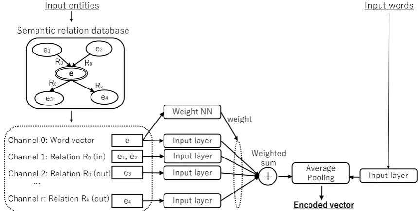
Figure 2: Our proposed method expands input entities using a KB, then entities are fed into input layers along with their relation names and directions. The vectors that are obtained from the input layers are combined via a weighted sum. The text associated with a user is also embedded, and a combined representation is generated based on average pooling with the entity embedding.

data set,Eis the set of entities in the KB,Ris the set of relations in the KB,T is the set of terms in the data set (the “vocabulary”),V is the union of the U andT (V = U ∪T), and dis the size of dimension for embedding.

Our method consists of two components: a text encoding, and a region prediction. We describe each component below.

3.1 Text encoding

To learn a vector representation of the text associ-ated with a user, we use a method inspired by rela-tional graph convolurela-tional networks (Schlichtkrull et al.,2017).

Our proposed method is illustrated in Figure2. Each channel in the encoding corresponds to a directed relation, and these channels are used to propagate information about the entity. For in-stance, the channel for (bornIn, BACKWARDS) can be used to identify all individuals born in a given location, which could provide a useful sig-nal, e.g., to find synonymous or overlapping re-gions in the data set. Our text encoding method is based on embedding the properties of each en-tity based on its representation in the KB, and its neighbouring entities.

Consider Tweets that user posted containing n

entity mentions {e1, e2, ..., en}, each of which is

contained in a KB,ei ∈E. The vectormeir ∈1 |d|

represents the entity ei based on the set of other

entities connected through directed relationr, i.e.,

meir=

X

e0_∈Nr(e

i)

W_e(1)0 , (1)

where, W_e(1)0 ∈ 1d is the embedding of entity e0

from embedding matrix W(1) ∈ R|V|×d _{, and}

Nr(e) is the neighbourhood function, which

re-turns all nodes e0 connected to e by directed re-lationr.

Then, meir for all r are transformed using a weighted sum:

vei =

X

r∈R

airReLU(meir)

~ai =σ(W(2)·~ei),

(2)

where,~ai∈1|R|is the attention that entityei

rep-resented by one-hot vector~ei pays to all relations

using weight matrixW(2) ∈ R|V|×|R|_{, andσ and}

ReLUare the sigmoid and the rectified linear unit activation functions, respectively. Here, we obtain entity embedding vectorvei ∈1

d_{for entitye} i.

Since the number of entities in tweets is sparse, we also encode, and use all the terms in the tweet regardless of if they are entity or not. We represent each term by:

vwj =W (1)_·w~

j, (3)

value j equals frequency ofwj in the tweet, and

W(1)is shared with entities (Equation1).1 Overall, user representation vectoruis obtained as follows:

u= 1

n+m 



n

X

i=1

vei+

m

X

j=1

vwj



 , (4)

wheremis the number of words that the user men-tioned.

Our method has two special features: sharing the weight matrix across all channels, and using a weighted sum to combine vectors from each chan-nel; these distinguish our method from R-GCN (Schlichtkrull et al.,2017). The reason we share the embedding matrix is that the meaning of the entity should be the same even if the relation type is different, so we consider that the embedding vector should be the same irrespective of relation type. We adopt weighted sum because even if the meaning of the entity is the same, if the entity is connected via different relation types, its func-tional semantics should be customized to the par-ticular relation type.

3.2 Region estimation

To estimate the location for a given user, we pre-dict a region using a 1-layer feed-forward neural network with a classification output layer as fol-lows:

o= softmaxW(3)u , (5)

whereW(3) ∈ Rclass×d _{is a weight matrix. The}

classes represent regions in the data set, defined using k-means clustering over the continuous lo-cation coordinations in the training set (Rahimi et al., 2017a). Each class is represented by the mean latitude and longitude of users belonging to that class, which forms the output of the model. The model is trained using categorical cross-entropy loss, using the Adam optimizer (Kingma and Ba,2014) with gradient back-propagation.

4 Experiments

4.1 Evaluation

Geolocation models are conventionally evaluated based on the distance (in km) between the known and predicted locations. Following Cheng et al.

(2010) andEisenstein et al.(2010), we use three evaluation measures:

1_{We consider words as a special case of entities, having}

no relations.

1. Mean: the mean of distance error (in km) for all test users.

2. Median: the median of distance error (in km) for all test users; this is less sensitive to large-valued outliers thanMean.

3. Acc@161: the accuracy of geolocating a test user within 161km (= 100 miles) of their real location, which is an indicator of whether the model has correctly predicted the metropoli-tan area a user is based in.

Note that lower numbers are better forMeanand

Median, while higher is better forAcc@161.

4.2 Data set and settings

We base our experiments on GeoText (Eisenstein et al., 2010), a Twitter data set focusing on the contiguous states of the USA, which has been widely used in geolocation research. The data set contains approximately 6,500 training users, and 2,000 users each for development and test. Each user has a latitude and longitude coordinate, which we use for training and evaluation. We exclude @-mentions, and filter out words used by fewer than 10 users in the training set.

We use Yago3 (Mahdisoltani et al.,2014) as our knowledge base in all experiments. Yago3 con-tains more than 12M relation edges, with around 4.2M unique entities and 37 relation types. We compare three relation sets:

1. GEORELATIONS: {isLocatedIn, livesIn,

diedIn,happenedIn,wasBornIn}

2. TOP-5 RELATIONS:{isCitizenOf, hasGen-der,isAffiliatedTo,playsFor,creates}

3. GEO+TOP-5 RELATIONS: Combined GEO -RELATIONSand TOP-5 RELATIONS

The first of these was selected based on rela-tions with an explicit, fine-grained location com-ponent,2while the second is the top-5 relations in Yago3 based on edge count.

We use AIDA (Nguyen et al., 2014) as our named entity recognizer and linker for Yago3.

The hyperparameters used were: a minibatch size of 10 for our method, and full batch for R-GCN methods mentioned in the following section;

2_{GrantedisCitizenOfis also geospatially relevant, but}

each component, text encoding and region estima-tion, has one layer; 32 regions;L2 regularization coefficient of10−5; hidden layer size of 896; and 50 training iterations, with early stopping based on development performance.

All models were learned with the Adam opti-miser (Kingma and Ba,2014), based on categori-cal cross-entropy loss with channel weightsWc=

|cmax|

|c| , where|c|is the number of entities of class typecappearing in the training data, and|cmax|is

that of the most-frequent class. Each layer is ini-tialized using HENormal (He et al.,2015), and all models were implemented in Chainer (Tokui et al.,

2015).

4.3 Baseline Methods

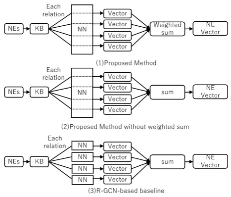
We compare our method with two baseline meth-ods: (1) the proposed method without weighted sum; and (2) an R-GCN baseline, over the same sets of relations as our proposed method. Both methods expand entities using the KB, which helps handle low-frequency and out-of-vocabulary (OOV) entities. Figure3illustrates the difference between the proposed and two baseline methods. The difference between these methods is only in the text encoding part. We describe these baseline methods in detail below.

Proposed Method without Weighted Sum

(“simple average”’): To confirm the effect of

the weighted sum in the proposed method, we use the proposed method without weighted sum as one of our baselines. Here, we usear = _|Nr1_(e

i)| in-stead ofairin Equation2.

R-GCN baseline method (R-GCN): The

R-GCNs we use are based on the method of

Schlichtkrull et al.(2017). The differences are in having a weight matrix for each channel, and us-ing non-weighted sum.

4.4 Results

Table1presents the results for our method, which we compare with three benchmark text-based user geolocation models from the literature (Cha et al.,

2015;Rahimi et al., 2015b, 2017b). We present results separately for the three relation sets,3 un-der the following settings: (1) implemented within our proposed method, (2) the proposed method

3_{Note that G}

EORELATIONSand TOP-5 RELATIONS in-clude five relation types, while GEO+TOP-5 RELATIONS in-cludes 10 relation types, so it is not fair between three rela-tion sets.

(1)Proposed Method

(3)R-GCN-based baseline KB NN

Vector Vector Vector Vector Each

relation

Weighted sum

NE Vector NEs

KB

NN Vector Vector Vector Vector Each

relation

sum _VectorNE

NEs NN

NN NN

(2)Proposed Method without weighted sum KB NN

Vector Vector Vector Vector Each

relation

sum _VectorNE NEs

Figure 3: The difference between the proposed and two baseline methods. The proposed method shares the weight matrix between the different channels. The first baseline is almost the same as the proposed method, with the only difference being that a simple sum is used instead of a weighted sum. The R-GCN baseline learns a separate weight matrix for each channel.

without weighted sum; and (3) R-GCN baseline method.

The best results are achieved with our pro-posed method using the GEO+TOP-5 RELA

-TIONS, in terms of both Acc@161 and Me-dian. The second-best results across these metrics are achieved using our proposed method without weighted sum using GEO+TOP-5 RELATIONS, and the third-best results are for our proposed method using GEORELATIONS. Surprisingly, R-GCN baseline methods perform worse that the benchmark methods in terms of Acc@161 and

Median. No method outperforms Cha et al.

(2015) in terms of Mean, suggesting that this method produces the least high-value outlier pre-dictions overall; we do not reportAcc@161 for this method as it was not presented in the original paper.

4.5 Discussion

Relation set Method Acc@161↑ Mean↓ Median↓

GEORELATIONS

Proposed method 43 780 339

without weighted sum 41 838 349

R-GCN 41 859 373

TOP-5 RELATIONS

Proposed method 41 807 354

without weighted sum 42 852 342

R-GCN 41 898 452

GEO+TOP-5 RELATIONS

Proposed method 44 821 325

without weighted sum 43 825 325

R-GCN 41 914 449

Cha et al.(2015) — 581 425

Rahimi et al.(2015b) 38 880 397

Rahimi et al.(2017b) 40 856 380

Table 1: Geolocation prediction results (“—” indicates that no result was published for the given combination of benchmark method and evaluation metric).

Used relation Acc@161↑ Mean↓ Median↓ Number of edges in Yago3

MLP (without relations) 40 856 380 —

+isLocatedIn 43 793 321 3,074,176

+livesIn 42 836 347 71,147

+diedIn 43 844 346 257,880

+happenedIn 43 831 328 47,675

+wasBornIn 42 821 328 848,846

+isCitizenOf 42 825 347 2,141,725

+hasGender 43 824 338 1,972,842

+isAffiliatedTo 42 832 352 1,204,540

+playsFor 43 807 322 783,254

+create 41 880 358 485,392

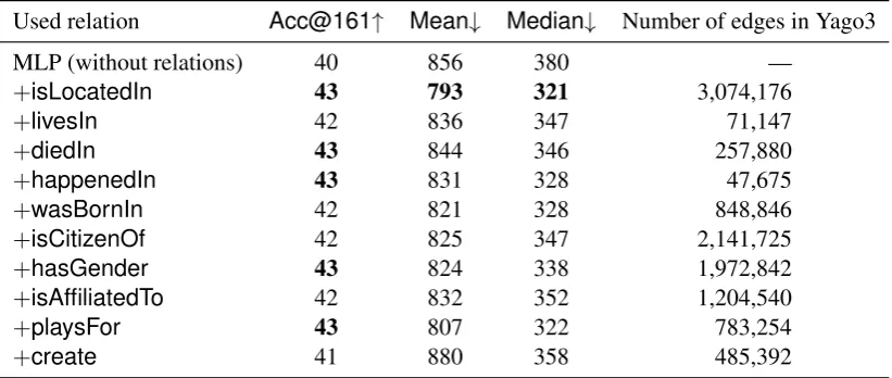
Table 2: Effect of each relation type.

that this is despite them being more sparsely-distributed in Yago3, and also that a more general-purpose set of relations also resulted in higher ac-curacy. The combination of geolocation-specific and general-purpose set (GEO+TOP-5 RELA

-TIONS) is the best result in the table, but the

im-provement from using only GEORELATIONS is limited. That is, even though our method works with general-purpose relation set, it is better to choose task-specific relations.

To confirm which relations have the greatest utility for user geolocation, we conducted an ex-periment based on using one relation at a time. As detailed in Table 2, relations that are better represented in Yago3 such as isLocatedIn and

playsForhave a greater impact on results, in part because this supports greater generalization over OOV entities. Having said this, the relation which

has the least edges,happenedIn, has the highest impact on results in term ofAcc@161 and the third impact in terms ofMeanandMedian show-ing that it is not just the density of a relation that is a determinant of its impact. Surprisingly, the over-all best result in terms ofMedian, which includes using relation sets such as GEORELATIONS and GEO+TOP-5 RELATIONS, is obtained by with is-LocatedInonly, despite it being a single relation. This result also shows that choosing task-specific relations is one of the important features in our method.

200 250 300 350 400 450

Proposed method R-GCN based method

Number of the unit of middle layer

896 672

448 224

112 Median error

Figure 4: Comparison of number of units in middle layer, in terms ofMedianerror.

0 100 200 300 400 500 600

Proposed BoW

1-39 (1,234)

40-59 (377)

60-79 (155)

80-99 (66)

100-(63) Median error

Number of Tweets per user in test set (Number of users)

Figure 5: Breakdown of results according to number of tweets per user, in terms ofMedian.

number of parameters, we conducted an experi-ment comparing theMedianerror as we changed the number of units in the middle layer in the range {112,224,448,672,896} for our proposed method and the R-GCN baseline method. As shown in Figure 4, the Median error of the R-GCN baseline method is almost equal when the number of units is between 224 and 896, at a level worse than our proposed method. This result sug-gests that the R-GCN baseline method cannot be improved by simply reducing the number of pa-rameters. This is because the amount of train-ing data is imbalanced for each channel, so some channels do not train well over small data sets. With larger data sets, it is likely that the R-GCN baseline would perform better, which we leave to future work.

We also analyzed the results across test users with differing numbers of tweets in the data set, as detailed in Figure 5, broken down into bins of 20 tweets (from 40 tweets; note that the min-imum number of tweets for a given user in the data set is 20). “Proposed” refers to our proposed

0 200 400 600 800 1000 1200

Proposed BoW

0 (719) Median error

1-2 (776)

3-5 (297)

6-9 (75)

10-(28)

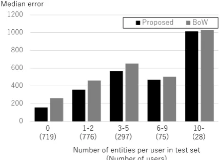
Number of entities per user in test set (Number of users)

Figure 6: Breakdown of results according to number of entities per user, in terms ofMedianerror.

method using GEORELATIONS, and “BoW” refers to the bag-of-words MLP method ofRahimi et al.

(2017b). We can see that our method is superior for users with small numbers of tweets, indicating that it generalizes better from sparse data. This suggests that our method is particularly relevant for small-data scenarios, which are prevalent on Twitter in a real-time scenario.

Figure6shows the results across test users with differing numbers of entities in the data set. Our method can improve for all cases, even users who do not mention any entities. This is because our method shares the same weight matrix for entity and word embeddings, meaning it is optimized for both. On the other hand, the median error for users who mention over 10 entities is high. Most of their tweets mention sports events, and they typically include more than two geospatially-grounded en-tities. For example,Lakers @ Bobcatshas two en-tities —LakersandBobcats— both of which are basketball teams, but their hometown is different (Los Angeles, CA for Lakers and Charlotte, NC forBobcats). Therefore, users who mention many entities are difficult to geolocate.

Tweets are written in colloquial style, making NER difficult. For this reason, it is highly likely that there is noise in the output of AIDA, our NE recognizer. To investigate the tension between precision and recall of NE recognition and linking, we conducted an experiment using simple case-insensitive longest string match against Yago3 as our NE recognizer, which we would expect to have higher recall but lower precision than AIDA. Table 3 shows the results, based on GEORELA

Method Acc@161↑ Mean↓ Median↓ Entities / User

AIDA 43 780 339 1.6

Longest string match 42 827 325 87.9

Table 3: Result for different named entity recognizers.

string match is superior in terms of Median de-spite its simplicity. Given its efficiency, and there being no need to train the model, this potentially has applications when porting the method to new KBs or applying it in a real-time scenario.

5 Conclusion and Future Work

In this paper, we proposed a user geolocation pre-diction method based on entity linking and em-bedding a knowledge base, and confirmed the ef-fectiveness of our method through evaluation over the GeoText data set. Our method outperformed conventional text-based geolocation, in terms of

Acc@161andMedian, due to its ability to gen-eralize over OOV named entities, which was seen particularly for users with smaller numbers of tweets. We also showed that our method is not re-liant on a pre-trained named entity recognizer, and that the selection of relations has an impact on the results of the method.

In future work, we plan to combine our method with user mention-based network methods, and to confirm the effectiveness of our method over larger-sized data sets.

References

Amr Ahmed, Liangjie Hong, and Alexander J Smola. 2013. Hierarchical geographical modeling of user locations from social media posts. InProceedings of the 22nd International Conference on World Wide Web, pages 25–36.

Zahra Ashktorab, Christopher Brown, Manojit Nandi, and Aron Culotta. 2014. Tweedr: Mining Twitter to inform disaster response. InISCRAM.

Timothy Baldwin, Paul Cook, Marco Lui, Andrew MacKinlay, and Li Wang. 2013. How noisy so-cial media text, how diffrnt soso-cial media sources? In Proceedings of the 6th International Joint Con-ference on Natural Language Processing (IJCNLP 2013), pages 356–364, Nagoya, Japan.

Timothy Baldwin, Marie-Catherine de Marneffe, Bo Han, Young-Bum Kim, Alan Ritter, and Wei Xu. 2015. Shared tasks of the 2015 Workshop on Noisy User-generated Text: Twitter lexical normalization and named entity recognition. InProceedings of the

ACL 2015 Workshop on Noisy User-generated Text, pages 126–135, Beijing, China.

Joan Bruna, Wojciech Zaremba, Arthur Szlam, and Yann Lecun. 2014. Spectral networks and lo-cally connected networks on graphs. In Inter-national Conference on Learning Representations (ICLR2014).

Shawn Brunsting, Hans De Sterck, Remco Dolman, and Teun van Sprundel. 2016. GeoTextTagger: High-precision location tagging of textual docu-ments using a natural language processing approach.

arXiv preprint arXiv:1601.05893.

Miriam Cha, Youngjune Gwon, and HT Kung. 2015. Twitter geolocation and regional classification via sparse coding. InICWSM, pages 582–585.

Zhiyuan Cheng, James Caverlee, and Kyumin Lee. 2010. You are where you tweet: a content-based ap-proach to geo-locating Twitter users. InProceedings of the 19th ACM International Conference on In-formation and Knowledge Management, pages 759– 768.

Ryan Compton, David Jurgens, and David Allen. 2014. Geotagging one hundred million Twitter accounts with total variation minimization. In 2014 IEEE International Conference on Big Data, pages 393– 401.

Micha¨el Defferrard, Xavier Bresson, and Pierre Van-dergheynst. 2016. Convolutional neural networks on graphs with fast localized spectral filtering. In Ad-vances in Neural Information Processing Systems, pages 3844–3852.

Tien Huu Do, Duc Minh Nguyen, Evaggelia Tsili-gianni, Bruno Cornelis, and Nikos Deligian-nis. 2017. Multiview deep learning for pre-dicting Twitter users’ location. arXiv preprint arXiv:1712.08091.

David K Duvenaud, Dougal Maclaurin, Jorge Ipar-raguirre, Rafael Bombarell, Timothy Hirzel, Al´an Aspuru-Guzik, and Ryan P Adams. 2015. Convolu-tional networks on graphs for learning molecular fin-gerprints. In Advances in Neural Information Pro-cessing Systems, pages 2224–2232.

Justin Gilmer, Samuel S Schoenholz, Patrick F Riley, Oriol Vinyals, and George E Dahl. 2017. Neural message passing for quantum chemistry. In Inter-national Conference on Machine Learning, pages 1263–1272.

Bo Han, Paul Cook, and Timothy Baldwin. 2012. Ge-olocation prediction in social media data by finding location indicative words. InProceedings of COL-ING 2012, pages 1045–1062, Mumbai, India.

Bo Han, Paul Cook, and Timothy Baldwin. 2014. Text-based Twitter user geolocation prediction. Journal of Artificial Intelligence Research, 49:451–500.

Bo Han, Afshin Rahimi, Leon Derczynski, and Timo-thy Baldwin. 2016. Twitter geolocation prediction shared task of the 2016 Workshop on Noisy User-generated Text. InProceedings of the 2nd Workshop on Noisy User-generated Text (WNUT), pages 213– 217.

Kohei Hayashi, Takanori Maehara, Masashi Toyoda, and Ken-ichi Kawarabayashi. 2015. Real-time top-r topic detection on Twittetop-r with topic hijack filtetop-r- filter-ing. InProceedings of the 21st ACM SIGKDD Inter-national Conference on Knowledge Discovery and Data Mining, pages 417–426.

Kaiming He, Xiangyu Zhang, Shaoqing Ren, and Jian Sun. 2015. Delving deep into rectifiers: Surpass-ing human-level performance on imagenet classifi-cation. In Proceedings of the IEEE International Conference on Computer Vision, pages 1026–1034.

Liangjie Hong, Amr Ahmed, Siva Gurumurthy, Alexander J Smola, and Kostas Tsioutsiouliklis. 2012. Discovering geographical topics in the Twit-ter stream. InProceedings of the 21st International Conference on World Wide Web, pages 769–778.

David Jurgens. 2013. That’s what friends are for: Infer-ring location in online social media platforms based on social relationships. ICWSM, pages 273–282.

Diederik P Kingma and Jimmy Ba. 2014. Adam: A method for stochastic optimization. arXiv preprint arXiv:1412.6980.

Thomas N Kipf and Max Welling. 2016. Semi-supervised classification with graph convolutional networks. arXiv preprint arXiv:1609.02907.

Michael D Lieberman, Hanan Samet, and Jagan Sankaranarayanan. 2010. Geotagging with local lexicons to build indexes for textually-specified spa-tial data. In26th International Conference on Data Engineering (ICDE 2010), pages 201–212.

Ji Liu and Diana Inkpen. 2015. Estimating user lo-cation in social media with stacked denoising auto-encoders. In Proceedings of the 1st Workshop on Vector Space Modeling for Natural Language Pro-cessing, pages 201–210.

Farzaneh Mahdisoltani, Joanna Biega, and Fabian Suchanek. 2014. Yago3: A knowledge base from multilingual wikipedias. In7th Biennial Conference on Innovative Data Systems Research.

Anshul Mittal and Arpit Goel. 2012. Stock prediction using Twitter sentiment analysis. Stanford Univer-sity, CS229.

Yasuhide Miura, Motoki Taniguchi, Tomoki Taniguchi, and Tomoko Ohkuma. 2017. Unifying text, meta-data, and user network representations with a neu-ral network for geolocation prediction. In Proceed-ings of the 55th Annual Meeting of the Association for Computational Linguistics (Volume 1: Long Pa-pers), volume 1, pages 1260–1272.

Junta Mizuno, Masahiro Tanaka, Kiyonori Ohtake, Jong-Hoon Oh, Julien Kloetzer, Chikara Hashimoto, and Kentaro Torisawa. 2016. WISDOM X, DIS-AANA and D-SUMM: Large-scale NLP systems for analyzing textual big data. In Proceedings of the 26th International Conference on Computational Linguistics: System Demonstrations, pages 263– 267.

Dat Ba Nguyen, Johannes Hoffart, Martin Theobald, and Gerhard Weikum. 2014. AIDA-light: High-throughput named-entity disambiguation. LDOW, 1184.

Gianluca Quercini, Hanan Samet, Jagan Sankara-narayanan, and Michael D Lieberman. 2010. De-termining the spatial reader scopes of news sources using local lexicons. In Proceedings of the 18th SIGSPATIAL International Conference on Advances in Geographic Information Systems, pages 43–52.

Afshin Rahimi, Timothy Baldwin, and Trevor Cohn. 2017a. Continuous representation of location for geolocation and lexical dialectology using mixture density networks. InProceedings of the 2017 Con-ference on Empirical Methods in Natural Language Processing, pages 167–176.

Afshin Rahimi, Trevor Cohn, and Timothy Baldwin. 2015a. Twitter user geolocation using a unified text and network prediction model. InProceedings of the 53rd Annual Meeting of the Association for Compu-tational Linguistics and the 7th International Joint Conference on Natural Language Processing (Vol-ume 2: Short Papers), pages 630–636.

Afshin Rahimi, Trevor Cohn, and Timothy Baldwin. 2017b. A neural model for user geolocation and lex-ical dialectology. InProceedings of the 55th Annual Meeting of the Association for Computational Lin-guistics (Volume 2: Short Papers), volume 2, pages 209–216.

Afshin Rahimi, Duy Vu, Trevor Cohn, and Timothy Baldwin. 2015b. Exploiting text and network con-text for geolocation of social media users. In Pro-ceedings of the 2015 Conference of the North Amer-ican Chapter of the Association for Computational Linguistics: Human Language Technologies, pages 1362–1367.

Bahar Salehi, Dirk Hovy, Eduard Hovy, and Anders Søgaard. 2017. Huntsville, hospitals, and hockey teams: Names can reveal your location. In Proceed-ings of the 3rd Workshop on Noisy User-generated Text, pages 116–121, Copenhagen, Denmark.

Michael Schlichtkrull, Thomas N Kipf, Peter Bloem, Rianne van den Berg, Ivan Titov, and Max Welling. 2017. Modeling relational data with graph convolu-tional networks. arXiv preprint arXiv:1703.06103.

Jianfeng Si, Arjun Mukherjee, Bing Liu, Qing Li, Huayi Li, and Xiaotie Deng. 2013. Exploiting topic based Twitter sentiment for stock prediction. In Pro-ceedings of the 51st Annual Meeting of the Associa-tion for ComputaAssocia-tional Linguistics (Volume 2: Short Papers), volume 2, pages 24–29.

Partha Pratim Talukdar and Koby Crammer. 2009. New regularized algorithms for transductive learn-ing. In Proceedings of the European Conference on Machine Learning (ECML-PKDD) 2009, pages 442–457, Bled, Slovenia.

Seiya Tokui, Kenta Oono, Shohei Hido, and Justin Clayton. 2015. Chainer: a next-generation open source framework for deep learning. InProceedings of the NIPS 2015 Workshop on Machine Learning Systems (LearningSys).

Jan Vosecky, Di Jiang, Kenneth Wai-Ting Leung, and Wilfred Ng. 2013. Dynamic multi-faceted topic discovery in Twitter. In Proceedings of the 22nd ACM International Conference on Information and Knowledge Management, pages 879–884.