Multistep Sparse Approximation Technology in Information Retrieval

Multistep Sparse Approximation Technology in

Information Retrieval

Chi Shen

400 E. Main Street Frankfort, KY 40601

Wen Li

740 W New Circle Rd Lexington, KY 40511

Mike F. Unuakhalu

400 E. Main Street Frankfort, KY 40601

ABSTRACT

With large sets of text documents increasing rapidly, being able to efficiently utilize this vast volume of new information and ser-vice resource presents challenges to computational scientists. Text documents are usually modeled as a term-document matrix which has high dimensional and space vectors. To reduce the high di-mensions, one of the various dimensionality reduction methods, concept decomposition, has been developed by some researchers. This method is based on document clustering techniques and least-square matrix approximation to approximate the matrix of vectors. However the numerical computation is expensive, as an inverse of a dense matrix formed by the concept vector matrix is required. In this paper we presented a class of multistep spare matrix strategies for concept decomposition matrix approximation. In this approach, a series of simple sparse matrices are used to approximate the de-compositions. Our numerical experiments on both small and large datasets show the advantage of such an approach in terms of stor-age costs and query time compared with the least-squares based approach while maintaining comparable retrieval quality.

General Terms:

Computer Information Retrieval

Keywords:

Term-document matrix, Concept decomposition matrix, Sparsity pattern, Multistep, Sparse matrix approximation

1. INTRODUCTION

The text retrieval method using Latent Semantic Indexing (LSI) with the low-rank Singular Value Decomposition (SVD) of the term-document matrix has been intensively studied for years [1, 9, 16]. Although the LSI method has empirical success, it suffers from the lack of interpretation for the low-rank approximation [6] and may be less effective for large heterogeneous text collections [9, 10]. A method introduced by [5] is an improvement in that di-rection. In this approach, a large amount of dataset is first parti-tioned into a set of disjoint clusters. The centroids of clusters or also known as concept decomposition is computed and normalized as the concept vector of that cluster for lowering the rank of the term-document matrix [6]. Gao and Zhang [7] have indicated that

retrieval accuracy from the concept decomposition can be compara-ble to that from LSI. However, the numerical computation based on the straightforward implementation of the concept matrix decom-position is expensive, as an inverse of the normal matrix (which is likely to be a dense matrix) formed by the concept vector matrix is required during the query procedure. The dense data structure of the concept decomposition matrix poses a huge challenge for both disk and memory spaces of conventional computers. Some researchers [2, 7, 11, 18] have recently applied sparsification techniques to re-duce computational cost and memory space of concept decompo-sition method. In [7] it proposed a sparsification strategy by drop-ping small entries during the concept matrix inverse computation. They have demonstrated that the sparsified concept decomposition technique may improve the performance in terms of retrieval ac-curacy and storage cost for some cases compared with SVD. The approach used in [11] is quite different from [7]. The LSI input matrices have been sparsified by identifying and removing some values from submatrices that are used in LSI methods. Shen and Williams [18] utilized the knowledge of both preconditioning tech-niques and the computational theorems to compute a sparse matrix to approximate the projection matrix directly. The key part in their approach is the sparsity pattern strategies. Different strategy pat-terns may result in quite different performance. This method based on different sparsity pattern strategies greatly reduces memory cost and query time while maintaining close retrieval accuracy to that of the straightforward implementation of the concept matrix decom-position method.

less CPU time and memory space required to compute the decom-position matrix and perform document retrieval.

This paper is organized as follows. Concept decomposition tech-niques and least squares matrix approximation based retrieval pro-cedures are discussed in Section 2 and Section 3. These are fol-lowed by a detailed discussion of the multistep sparse matrix ap-proximation based strategies in Section 4. Numerical experiments are presented in Section 5. We summarize this paper in Section 6.

2. DOCUMENT CLUSTERING AND CONCEPT VECTORS

In information retrieval, text documents are modeled as a term-document matrix whose rows are the terms and columns are doc-ument vectors. Suppose we are given the set of docdoc-ument vectors

Am×n = [a1, a2, . . . , an],whereaj,(j= 1,2, . . . , n)is thejth document vector ofm dimension in the collection. Usually, the term-document matrices are high dimensional as each data set may contain thousands of words and are very sparse, with 1-5% or less terms in each document.

We first partition the documents intokdisjoint clusters{πj}kj=1by usingk-means or other clustering algorithms such that

k

[

j=1

πj={a1, a2, . . . , an} and πj∩πi=φ if j6=i.

For each fixedj,1≤j≤k, the centroid vector of each cluster is defined as

e

cj=

1

nj

X

ai∈πj

ai,

wherenj = |πj|is the number of documents in clusterπj. The centroid vectors are normalized in following

cj= e

cj

kc_ejk

, j= 1,2, . . . , k.

An intuitive definition of the clusters is that, ifai∈πj, then

aT

icj> aTicl for l= 1,2, . . . , k, l6=j,

i.e., documents inπjare closer to its centroid than to the other cen-troids. If the clustering is not good enough, a new set of centroid vectors for the new partitioning is computed. Each document will be reassigned to a new cluster based on the new computed centroid vector. This process can be repeated a few times to a stopping threshold value ofne. If each cluster is compact enough, the cen-troid vector may represent the abstract concept of the cluster. So they are also calledconcept vectors[5]. Theconcept matrixcan be defined as anm×kmatrix such that,

C= [c1, c2, . . . , ck].

The concept matrixCthat has rankm×kis still a sparse matrix, as each columncjis sparse. This is becausecjis a group of docu-ments inAwith similar key words, i.e. the columns ofAthat have similar number of non-zeros at almost the same fill-in positions. Due toA’s sparsity,cjis sparse too. The degree of sparsity ofCis inversely proportional to the number of clusters generated. If we as-sume that the concept vectors are linearly independent, the concept matrix has rankk.

For any partitioning of the document vectors, we can define the cor-responding concept decompositionA˜of the term-document matrix

Aas the least squares approximation ofAonto the column space

of the concept matrixC. We write the concept decomposition as an

m×nmatrix

˜

A=CM ,˜

whereM˜ is ak×nmatrix that is to be determined by solving the following least squares problem

˜

M = arg min

M kA−CMk

2

F. (1)

Here the normk · kF is the Frobenius norm of a matrix. It is well-known that problem (1) has a closed-form solution, i.e.,

˜

M= (CT_C)−1_CT_A.

(2)

3. RETRIEVAL PROCEDURE AND

APPROXIMATE LEAST SQUARES BASED STRATEGIES

As it had been described in [8, 18], given a query vectorq, the retrieval with the concept projection matrix (CPM)A˜can be com-puted as

rT_=qT_A˜=qT_C(CT_C)−1_CT_{A, (3)}

whererT _{is the ranking vector. After sorting the entries ofr}T _in a descending order, we have a ranking list of documents which are related to the query (listed from the most relevant to the least rel-evant). The retrieval procedure in Eq. (3) is not efficient in terms of numerical computation and storage when the number of cluster

kis large as it needs to compute(CT_C)−1_{, which is likely to be a} dense matrix.

To make the numerical computation procedure and storage cost more competitive, a sparse matrix approximation technique based on the static and dynamic sparsity pattern strategies has been stud-ied in [18]. In this method, a sparse matrixMis computed to solve the least squares problem (1) approximately. That is to find a sparse matrixMsuch that the functionalf(M) =kA−C Mk2

F is min-imized, or more precisely,approximately minimized. In [18], static and dynamic sparsity pattern strategies had been discussed. In their numerical experiments, both of the approaches greatly reduced the computational costs and storage costs. Compared to the straight-forward implementation of concept matrix decomposition method CPM, both strategies use less than 5% memory storage of the CPM approach while achieving comparable retrieval accuracy.

Obviously there is much room to improve the sparsity pattern strategies. To have more accurate sparse approximate matrix, it is natural to think of increasing the sparsity ratio for M. However, the CPU time used for matrix M construction increases as well. Dynamic sparsity pattern strategies can compute better sparse ap-proximate matrix, given a certain sparsity ratio forM. However, they are usually expensive. In this paper we propose a multistep matrix approximation strategy based on static sparsity pattern ap-proach. At each step, we compute a series of sparse, or cheap matrix

Mi, i= 1,2, . . .at each step. Then the sum of these sparse

matri-ces is used to approximate the matrixM. This method takes the advantage of cheaper construction at each step and a denser matrix we will obtain at last.

4. MULTISTEP STATIC SPARSITY PATTERN APPROACH (MSSP)

In our problem in information retrieval, all we want is to find a

f(M) = min

M∈GkA−CMk

2

F, (4)

is minimized with certain constraints onM. This problem is simi-lar to that in the equation in preconditioning field:

f(M) = min

M∈GkI−AMk

2

F, (5)

Several sparse approximate inverse methods for solving above equation have been developed in [4, 17]. We will use these tech-nologies for our problem.

4.1 Computational procedure

For a moment, we suppose that a sparsity pattern setG forM is given somehow, the minimization problem (4) is decoupled inton

independent subproblems as

kA−CMk2

F =

n

X

j=1

k(A−CM)ejk22= n

X

j=1

kaj−Cmjk22, (6)

whereajand mj are thejth column of the matricesA andM, respectively. (ej is the jth unit vector.) It follows that the min-imization problem (6) is equivalent to minimizing the individual functions

kCmj−ajk2, j= 1,2, . . . , n, (7)

with certain restrictions placed on the sparsity pattern ofmj. In other words, each column ofM can be computed independently. This certainly opens the possibility for parallel implementation. Since we assume the sparsity pattern ofmj(andM) is given, i.e., a few, sayn2, entries ofmjat certain locations are allowed to be nonzero, the rest of the entries ofmjare forced to be zero. De-note then2nonzero entries ofmjbym¯jand then2columns ofC corresponding tom¯jbyCj. SinceCis sparse, the submatrixCj has many rows that are identically zero [4, 17]. After removing the zero rows ofCj, we have a reduced matrixC¯jwithn1rows. The individual minimization problem (7) is reduced to a much smaller least squares problem of ordern1×n2

k_C¯_{jm¯j−¯ajk2, j= 1,2, . . . , n, (8)}

in which¯ajconsists of the entries ofajcorresponding to the re-maining columns ofCj. We note that the matrixC¯jis now a very small rectangular matrix. It has full rank if the matrixCdoes. There are a variety of methods available to solve the small least squares problem (8). Assume thatC¯j has full rank. SinceC¯j is small, the easiest way is probably to perform a QR factorization on

¯

Cjas

¯

Cj=Qj

Rj

0

, (9)

whereRjis a nonsingular upper triangularn2×n2matrix.Qjis ann1×n1 orthogonal matrix, such thatQ−j1 = Q

T

j. The least squares problem (8) is solved by first computing¯cj =QTj¯ajand then obtaining the solution asm¯j =R−j1¯cj(1 :n2).In this way,

¯

mjcan be computed for eachj= 1,2, . . . , n, independently. This yields an approximate decomposition matrixM, which minimizes

kCM−AkF for the given sparsity pattern.

4.2 Multistep approach

From the above discussion, we can see that our computational pro-cedure is quite similar to that in [4, 17]. However it is much more

difficult than that in the preconditioning field. This is because of the fact thatAis am×nmatrix, not a square matrix. The dimensions of the matrixCand those ofMdo not match. That isCis am×k

matrix andMis ak×nmatrix. This multistep knowledge from the preconditioning field can not be directly applied to our application. We approach the problem for non-square matrix minimization in another way.

Suppose a simple and cheap sparsity pattern is chosen forM1.M1 is computed approximately for the equation

CM =A (10)

by using our modified sparse approximate inverse techniques de-veloped in [18]. IfCM1is not close enough toA, we can compute another approximate sparse matrixM2for the equation

CM=A−CM1 (11)

Based on Eq.( 11),CM2 ≈A−CM1, we sum the two matrices

M1andM2, such thatC(M1+M2)≈A. Generally,C(M1+M2) should be closer toAthanCM1does. IfC(M1+M2)is not good enough for the matrixA, we can compute the third sparse matrix

M3for the equation

CM =A−C(M1+M2) (12)

such thatC(M1 +M2+M3) ≈ A. This procedure can be re-peated for a few times to obtain a sequence of sparse matrices

M1, M2, ..., Ml such that C(M1 +M2 +...+Ml) ≈ A. As

[17] pointed out a few sparse matricesMlMl−1. . . M1for matrix approximate inverse may be capable of holding more information than a single matrixMcan. In our application, if eachMiis good in some sense, we expect that

lim

l−>∞C(M1+M2+...+Ml) =A

In general, the more accurate is matrixM, the more dense it is. Hence the computational cost may also increase. In our approach, since we sum the matrices at each step, it shouldn’t have many new fill-ins. For example, if the number of nonzeros of the matrixM1is

n1, and the number of nonzeros of the matrixM2isn2, the number of nonzeros of the matrixM1+M2would be less thann1+n2. IfM1 andM2 have the same sparsity patterns, there would be no new fill-ins. To avoid too few new fill-ins at each step, we choose different sparsity patterns forM1andM2.

We first define the sparsity pattern forM1. Note that the concept matrixCdescribes the relationship between the term vectors and the concept vectors. If a term is related to a concept vector, this relationship may be maintained in the approximate decomposition matrix in some sense. The strategy based on the sparsity pattern of

Cand entry values of bothCandAis described below. From the equationCM1 =A, we know thatcim

(1)

j =aij, where

ciis theith row ofC,m (1)

j is thejth column ofM1. The sparsity pattern ofm(1)_j is given in this way: Ifaijis the largest entry in the

jth column ofA, the sparsity pattern ofm(1)_j is the same as that of

ci. Here we use small matrices to illustrate our ideas. Suppose the three matrices areC4×3,M13×5andA4×5. The pattern ofCM1=

Ais depicted by the Eq (13).



 

x 0 x

0 x 0

x x 0

0 x 0 

 

4×3

− − − − − − − − − − − − − − −

!

= 

 

0 x 0 x 0 0 0 0 x x x x 0 0 0

x 0 x 0 0



 

4×5

(13)

Here, ”x” denotes nonzero entry, ”-” denotes undefined pattern. We determine the sparsity pattern ofM1column by column. First, find the largest entry in each column ofA, suppose they area31,

a12, a43, a14, and a25 in Eq (13). Then the sparsity pattern of

m(1)1 , is the same as that ofc3and the sparsity pattern ofm (1) 2 is the same as that ofc1,m(1)₃ has same sparsity pattern ofc4 and

m(1)₄ is the same as that ofc1. Finally we have the sparsity pattern

ofM1like this:

x x 0 x 0

x 0 x 0 x

0 x 0 x 0 !

.

For the sparsity pattern of matrixM2at the second step, we con-sider the equationCM2=A−CM1. We first sort non-zero entries in each column ofA−CM1. Then we go through all the entries from the largest to the smallest. Then the firstnenumber of largest entries will be used as new fill-ins forM2. If the positions of these selected entries have been used in matrixM1, these entries will continue to be used in the sparsity pattern inM2, but they are not counted as new fill-ins. So other larger entries will be selected to reach the totalnenumber of new fill-ins. A parameterneis used to control the number of new fill-ins for each column ofMiat theith step. So in general the matrixMiis denser thanMi−1. We had

con-ducted some numerical tests for this strategy. With a few new fill-ins for the matrixM2, the 2-norm residual ofkA−C(M1+M2)k2 reduces much more than that ofkA−C(M1+M2)k2with no more new fill-ins inM2. That means the denser matrixM1+M2may hold more information. This multistep procedure may be repeated for a few times as needed.

5. NUMERICAL EXPERIMENTS

In this section, we conducted some experiments to compare the per-formance of our proposed algorithms MSSP and the single-step ap-proximate sparse approach SSP and CPM method that is based on the straightforward implementation by solving Eq.( 2). Three small text databases: CRAN,MED and CISI and two large databases: LISA and NPL are used to validate our approach. The information about the five databases are given in Table 1.

Precision-recall curves are often used to evaluate the performance of the algorithms in information retrieval [15]. In the following ex-periments, we first test the precision-recall curves for different ap-proaches. We average the precision of all queries at fixed recall val-ues as10%,20%, . . . ,90%. Then we compare their storage costs by listing the number of nonzeros of the approximate matrixM ob-tained in Eq. (2). The CPU time required for the approximate ma-trix computation and query procedure is also reported for the tests over small datasets. The sparse matrix multistep computations are based on ParaSails developed in [4] by using C. This computation procedure and matrix inverse for concept project matrix method (CPM) were carried out in IBM Power/Intel(Xeon) hybrid system at University of Kentucky. The computations for query procedure were carried out in a SunOS system by using matlab.

In all the following tests, “nstep” denotes the number of steps used in sparse matrixMconstruction; “k” is the number of clusters used ink-mean algorithm; “nnz” represents the number of nonzeros for the matrixMconstructed with different methods. “ne”, a threshold value, is the number of new fill-ins in each column ofM at each step. As it was discussed in Section 4, the sparsity pattern of each

0 0.1 0.2 0.3 0.4 0.5 0.6 0.7 0.8 0.9

0 0.05 0.1 0.15 0.2 0.25 0.3 0.35 0.4

Precision

Recall

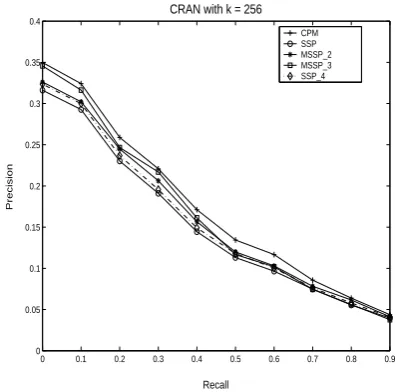
CRAN with k = 256

CPM SSP MSSP_2 MSSP_3 SSP_4

Fig. 1. Precision-Recall Results for CRAN withk= 256

column of matrixM depends on the number of the largest entries selected in the corresponding column ofA. The parameter “ne” means the firstnenumber of largest entries in each column ofA

that have not been used in the previous step will be selected . The larger the number ofne, the more dense is the matrix ofM. This usually leads to more accurate matrixM, and more computational and memory costs. This is because the storage space for the MSSP is primarily determined by the number of largest entries considered at each step. To balance the accuracy and the costs, in our tests we choosene = 2for multistep approach. In order to compare our multistep approach with the single-step SSP more precisely, we increase the density of SSP by settingne= 4. We denote it as “SSP 4”.

We first test the precision-recall curves for the CRAN database with

k= 256. As expected in Fig. 1, CPM has best query results. This is because CPM matrix is constructed by directly solving the Eq. (2). The resulting matrix is very dense(we will show this in the later tests) and hence more accurate than that of the other approximate approaches. From the Fig. 1 we can see the multistep algorithm MSSP withnstep = 2,3which does outperform the single-step approach SSP. This is partially because of more dense matrix con-structed in multistep approach. However more dense matrix doesn’t always generate more accurate matrix. Table 2 lists the numbers of nonzeros ofMconstructed with different approaches. Looking into our two-step approach MSSP that utilizes 2 largest entries for each column at each level and the single-step SSP that using 4 largest en-tries from the Table 2, we find that the SSP 4 constructs more dense matrix than MSSP. But in Fig. 1 we observe that 2-step MSSP has better retrieval accuracy than that of single-step SSP 4. That means with the same amount of memory cost, multistep approach usually construct more accurate matrix. This encouraging finding is what allowed us to intensify our efforts in developing multistep methods. We also make comparison of a 3-step MSSP and CPM. In Fig. 1 and Table 2 we found that the precision-recall curve for MSSP with

nstep= 3is very close to that of the CPM approach while 3-step

Table 1. The information of databases

Database Matrix size Number of queries

CISI 5,609×1,460 112

CRAN 4,612×1,398 225

MED 5,831×1,033 30

LISA 17,482×6,004 35

NPL 11,380×11,429 93

Table 2. Storage costs for CRAN database,k= 256 Methods ne nstep nnz

SSP 2 1 45,719

MSSP 2 2 75,986 SSP 4 4 1 93,878 MSSP 2 3 86,761 CPM - - 357,888

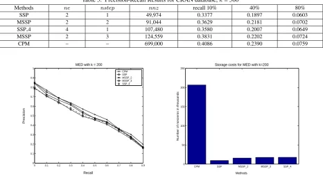
The test results listed in Table 3 are from testing the same database with the number of clusters:k= 500. Table 3 shows that the 2-step MSSP has better query results while using less memory space than SSP 4 approach. The data listed in the last two rows of Table 3 are the query results and nonzeros for the matrixM of 3-step MSSP and CPM. In this case, 3-step MSSP approach uses only 18% of CPM storages to achieve 93% retrieval accuracy of CPM. From this experiment, we also observe that the computational cost and query time have been greatly reduced.

Fig. 2 gives both query results and storage costs for testing the database MED withk= 200. From the left panel of Fig. 2, MSSP

withnstep = 3has really close query accuracy to that of CPM

approach. From the right panel of Fig. 2, we see that 3-step MSSP consumes only8%of storage space of CPM. This is because the dense matrix of CPM may have many noise entries. Our sparsifi-cation algorithm is designed to drop those unnecessary entries and keep very few entries that may hold more important information in the matrix. However it is difficult to predetermine those nonzero entries or sparsity pattern before solving the problem. This is still a challenging work in scientific field. We have tried to drop some small entries from CPM matrix. We found out that the query pre-cisions are also degraded and it still uses more than 10 times of storage than the 2-step MSSP matrix with comparable query accu-racy. This experiment again assures that a larger number of steps leads to better performance in terms of memory costs and compet-itive query precision.

We give the test for the dataset CISI. The query results, memory costs are given in Fig. 3. In this test, the multistep approach MSSP has slightly better performance than single step approach SSP and SSP 4 in terms of query precisions, query time and memory costs. Again, the higher values ofnstep, ornelead to more work, more fill-in inM matrix , and usually more accurate matrix. From the case reported in previous tests, we think that 2 or 3 steps MSSP is a good compromise between reasonable computational cost and comparable performance in terms of query precision.

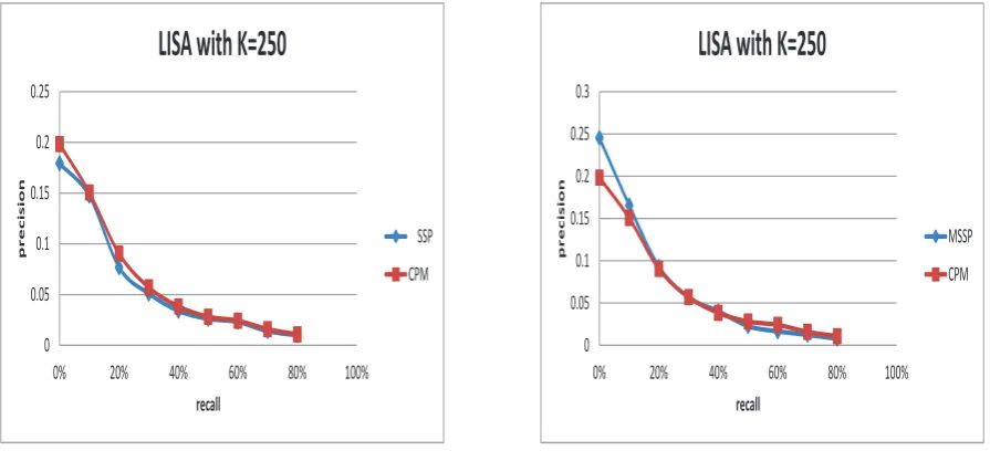
Below are the tests over two large datasets LISA and NPL. We first test the precision-recall curves and storage costs for the LISA database withk= 250.

Fig. 4 shows that our multistep algorithms have very close precision results to the one of CPM algorithm. However from the Fig. 5, we see the multistep algorithms that use much less memory spaces, about 50%, than that of CPM.

0 200000 400000 600000 800000 1000000 1200000 1400000 1600000

CPM SSP MSSP, nstep

n

u

m

b

e

r

o

f

n

o

n

z

e

r

o

s

algorithms

Storage for LISA with k = 250

Fig. 5. Storage costs for LISA withk= 250

From above results, we also observe that compared with the single-step strategy, the multisingle-step strategy can produce higher precision result. This is because the matrix constructed by MSSP may hold more information than the one constructed by SSP. However, as we stated earlier, denser approximate matrix may not always lead to better performance. Besides, the threshold value ofneis very es-sential during the construction of theM, so we use different thresh-old values to adjust the information held inM.

The test on LISA dataset has shown the advantages of the multi-step algorithms over CPM method. When we performed the NPL dataset, the results were mixed.

The above two figures in Fig. 6 are the precision-recall curves of NPL when it has been grouped into 500 clusters. A close observa-tion of the two curves shows a much better result in left panel over right panel of Fig. 6 in spite of its higher nonzero entries. See the storage costs in Fig. 5. Therefore, from this example, we can fur-ther conclude that in MSSP the denser approximate matrixMmay not achieve better performance due to potential noisy data that are captured in the denser matrix.

However, for NPL dataset, MSSP is not as robust as for LISA for different numbers of clusters. We tested NPL withk = 800in Fig. 8 and it shows that our MSSP is not comparable with CPM. Compared with the methods used in [13, 12, 14, 3], the size of NPL preprocessed in our way is much larger and the data matrix has the feature ofm < n, i.e. the document’s number is more than the term’s number. We think that MSSP does not work well due to some specific features of NPL.

6. CONCLUSION

Table 3. Precision-Recall Results for CRAN database,k= 500

Methods ne nstep nnz recall 10% 40% 80%

SSP 2 1 49,974 0.3377 0.1897 0.0603

MSSP 2 2 91,044 0.3629 0.2181 0.0702

SSP 4 4 1 107,480 0.3580 0.2007 0.0649

MSSP 2 3 124,559 0.3831 0.2202 0.0724

CPM – – 699,000 0.4086 0.2390 0.0759

0 0.1 0.2 0.3 0.4 0.5 0.6 0.7 0.8 0.9

0 0.1 0.2 0.3 0.4 0.5 0.6 0.7 0.8 0.9 1

Precision

Recall MED with k = 200

CPM SSP MSSP_2 MSSP_3 SSP_4

CPM SSP MSSP_2 MSSP_3 SSP_4

0 50 100 150 200 250

Storage costs for MED with k=200

Number of nonzeros in thousands

Methods

Fig. 2. Left panel: Query results for MED with k=200. Right panel: Storage costs for MED with k = 200.

0 1000000 2000000 3000000 4000000 5000000 6000000 7000000

CPM MSSP_3 MSSP_2

n

u

m

b

e

r

o

f

n

o

n

z

e

r

o

s

algorithms

Storage for NPL with k = 500

Fig. 7. Storage costs for NPL withk= 500

MSSP than CPM method. To compare our multistep MSSP with the single-step approach SSP under the constraint of the same amount of memory cost, we allow more nonzero entries (this can be con-trolled by adjusting the parameterne) at the first step of the SSP sparse matrix construction phase. Our numerical experiments have demonstrated that SSP can compute more dense matrix, but may not be more accurate compared with the multistep approach. Addi-tionally, MSSP is cheaper in its matrix computation phase as

evi-denced at each step of MSSP which resulted in a more sparse ma-trix. As was indicated in [17], computing a series of small memory cost (sparse) matrices usually cheaper than computing a high mem-ory cost (dense) matrix.

Although in our study, the performance of MSSP on NPL is not as good as it is on LISA and other small datasets, the advantages of MSSP in saving CPU memory space and computational costs have still been demonstrated. The best precision result of MSSP on NPL can be comparable with that in [14].

The multistep matrix approximation approach developed in this paper has provided a new avenue to approximate the concept de-composition matrix more cheaply and fast. If the storage cost and query time are the bottle-necks during the query procedure, this approach looks more attractive. There is much room for improve-ment. In our next step, the algorithm parallelism will be our first target. Due to the nature of the algorithm described in the paper, it will certainly open the door for the parallelism during the ma-trix approximation process. We then test it on some real larger cor-pora, like OHSUMED and some collections from TREC to better understand the performance of this approach. We also hope this multistep sparse matrix approximation approach may be applied to the general nonsquare sparse matrix approximation techniques for functional minimizationf(M) = minkA−CMk2

F. 7. REFERENCES

[1] M.Berry and M.Browne. Understanding Search Engines: Mathematical modeling and text retrieval.SIAM,1999 [2] C.M.Chen, N.Stoffel, M.Post, C.Basu, D. Bassu, and

0 0.1 0.2 0.3 0.4 0.5 0.6 0.7 0.8 0.9 0

0.05 0.1 0.15 0.2 0.25 0.3 0.35 0.4 0.45

Precision

Recall CISI with k = 500

CPM SSP MSSP_2 MSSP_3 SSP_4

CPM SSP MSSP_2 MSSP_3 SSP_4

0 100 200 300 400 500 600 700 800

Storage costs

Number of nonzeros in thousands

Methods

Fig. 3. Left panel: Query results for CISI with k=500. Right panel: The Storage costs.

0 0.05 0.1 0.15 0.2 0.25

0% 20% 40% 60% 80% 100%

p

r

e

c

i

s

i

o

n

recall

LISA with K=250

SSP

CPM

0 0.05 0.1 0.15 0.2 0.25 0.3

0% 20% 40% 60% 80% 100%

p

r

e

c

i

s

i

o

n

recall

LISA with K=250

MSSP

CPM

Fig. 4. Precision-recall for LISA withk= 250Left panel: CPM and SSP. Right panel: CPM and MSSP with 3 steps.

[3] J. Chen and Y. Saad. Divide and Conquer Strategies for Ef-fective Information Retrieval,Proceedings of the Ninth SIAM International Conference on Data Mining (SDM), 2009. [4] E. Chow. A priori sparsity patterns for parallel sparse

ap-proximate inverse preconditioners. SIAM J. Sci. Comput., 21(5):1804–1822, 2000.

[5] I. S. Dhillon and D. S. Modha. Concept decompositions for large sparse text data using clustering. Machine Learning, 42(1):143–175, 2001.

[6] J.Dobsa and B.J. Basic. Concept decomposition by fuzzy k-means algorithm, InProceedings of IEEE Web Intelligence Conference (WI2003), pp. 684-688, October 2003

[7] J. Gao and J. Zhang. Text retrieval using sparsified concept decomposition matrix. Book Chapter of Computational and Information Science, Springer Berlin/Heidelberg, vol. 3314, pp. 523 – 529, 2005

[8] J. Gao and J. Zhang. Clustered SVD strategies in latent se-mantic indexing. in Information Processing and Manage-ment, 41(5):1051-1063, 2005.

[9] P. Husbands, H. Simon, and C. Ding. On the use of singular value decomposition for text retrieval. In M. W. Berry, editor, Computational Information Retrieval, pages 145–156. SIAM, Philadelphia, PA, 2001.

[10] E. R. Jessup and J. H. Martin. Taking a new look at the la-tent semantic analysis approach to information retrieval. In Proceedings of the SIAM Workshop on Computational Infor-mation Retrieval, Raleigh, NC, 2000.

[11] A.Kontostathis, W.M.Pottenger, and B.D.Davison. Identi-fcation of critical values in Latent Semantic Indexing (LSI). Book chapter of Foundations of Data Mining and Knowledge Discovery, pp.333-346, 2005.

In-0 0.1 0.2 0.3 0.4 0.5

0% 20% 40% 60% 80% 100%

p

r

e

c

i

s

i

o

n

recall

NPL with K=500

MSSP

CPM

Fig. 6. Precision-recall for NPL withk= 500Left panel: CPM and MSSP with 2 steps. Right panel: CPM and MSSP with 3 steps.

0 0.1 0.2 0.3 0.4 0.5 0.6

0% 20% 40% 60% 80% 100%

p

r

e

c

i

s

i

o

n

recall

NPL with K=800

MSSP

CPM

0 2000000 4000000 6000000 8000000 10000000

CPM MSSP_3

n

u

m

b

e

r

o

f

n

o

n

z

e

r

o

s

algorithms

Storage for NPL with k = 800

Fig. 8. Left panel:Precision-recall for NPL withk= 800and 3 steps. Right panel: Storage costs for NPL withk= 800.

formation Processing and Management, 42(1):56-73, 2006. [13] A. Kontostathis, W.M. Pottenger, and B.D.Davison.

Identifi-cation of critical values in Latent Semantic Indexing(LSI).In Foundations of Data Mining and Knowledge Discoverypp. 333-346, 2005.

[14] A. Kontostathis. Essential Dimensions of Latent Semantic In-dexing (LSI). 40th Annual Hawaii International Conference on System Sciences, pp. 73, 2007.

[15] V.Raghavan, P.Bollmann, and G.S.Jung. A critical investi-gation of recall and precision as measures of retrieval sys-tem performance.ACM Transactions on Information Systems, Vol.7, pp.205-229, 1989.

[16] C.Tang, S.Dwarkadas, and Z.Xu. On scaling latent semantic indexing for large peer-to-peer systems.In Proceedings of the 27th Annual International ACM SIGIR Conference, Sheffield, UK, 2004

[17] K.Wang and J.Zhang. MSP:A class of parallel multistep suc-cessive sparse approximate inverse preconditioning strategies. SIAM Journal on Scientific Computing, Vol. 24, No.4, pp. 1141-1151, 2003