BIROn - Birkbeck Institutional Research Online
Chandna, Swati and Walden, A. (2011) Statistical properties of the estimator
of the rotary coefficient. IEEE Transactions on Signal Processing 59 (3), pp.
1298-1303. ISSN 1053-587X.
Downloaded from:
Usage Guidelines:
Please refer to usage guidelines at
or alternatively
Statistical Properties of the Estimator of the Rotary Coefficient
S. Chandna and A. T. Walden,Member, IEEE
Abstract— Rotary spectral analysis is a widely-used technique for studying elliptical motions in ocean currents, wind, etc. Sta-tistical properties (distribution, bias, confidence intervals) for the estimated rotary coefficient, which measures the tendency to rotate in a counterclockwise or clockwise manner, are derived and applied to ocean current measurements at six depths in the Labrador Sea.
Keywords— Complex-valued processes, confidence intervals, probability density function, rotary spectral analysis, rotary co-efficient.
I. Introduction
The analysis of two-component real-valued time series,{Xt}
and{Yt},with power spectraSX(f) andSY(f) respectively, can
be carried out by studying the real-valued vector time series or by considering the complex-valued series Zt = Xt+ iYt. The
latter approach is widely used in optics, quantum mechanics, electro-magnetics and communications [25], and particularly in physical sciences such as oceanography [6], meteorology [9], [12], [19] and geophysics [2]. The decomposition of the complex-valued series into polarized components, well-summarized in [23], [25], provides the added value of this approach in these sciences; in the frequency domain, the methodology is usually referred to as ‘rotary spectral analysis.’
Another major practical advantage is that several useful statistics are invariant to coordinate rotation under the rotary scheme. One of these is the rotary coefficient which we shall study in this article. Consider the following. A zero-mean co-variance stationary complex-valued random sequence is harmo-nizable, so
Zt=
1/2
−1/2
ei2πf tdZ(f), (1)
where Z(f) is a random function of f with uncorrelated in-crements, and zero mean. At frequencies f and −f the con-tribution to Zt is dZ(f)ei2πf t+ dZ(−f)e−i2πf t which is the
parametric equation of a random ellipse, comprising the addi-tion of two oppositely rotating circular moaddi-tions [6, pp. 428-9]. The counterclockwise component is considered to be rotating with positive frequency, and vice versa. Depending on which of the two components has the largest magnitude, the complex vector rotates clockwise or counterclockwise with time, with its tip tracing an ellipse. It is then natural to consider the rotary coefficient, defined as [6, p. 431],[7],
ρ(f) =SZ(f)−SZ(−f)
SZ(f) +SZ(−f)
, (2)
whereSZ(·) is the power spectrum for the process{Zt}defined
via E{dZ(f)dZ∗(f)} = η(f−f)SZ(f)df, where η(·) is the
Dirac delta train with period 1 [4, p. 505]. The rotary coef-ficient satisfies −1 ≤ρ(f) ≤1 and measures the tendency to rotate in a counterclockwise or clockwise manner; it provides an objective means of quantifying the rotation associated with the
Swati Chandna and Andrew Walden are both at the Department of Math-ematics, Imperial College London, 180 Queen’s Gate, London SW7 2BZ, UK. e-mail: [email protected] and [email protected]
asymmetry of the spectrum and is directly related to the ex-pected ellipse shape [25, p. 210]. Letf >0.Then ifρ(f) = +1, (i.e., SZ(−f) = 0), then motion is all counterclockwise
circu-lar at that frequency, whereas ifρ(f) =−1,(i.e.,SZ(f) = 0),
then motion is all clockwise circular at that frequency, and if ρ(f) = 0,then there is rectilinear motion (unidirectional flow). To immediately illustrate the very different physical insights gained from the real-valued or complex-valued view of two-component time series, we shall make use of ocean current speed and direction time series recorded at a mooring in the Labrador Sea [10], [11]. We associate the eastward (zonal) measurement of current speed with{Xt}and the northward (meridional)
mea-surement with {Yt}.Fig. 1(a) shows estimated spectra ˆSX(f)
(thin line) and ˆSY(f) (thick line) for {Xt} and {Yt},
respec-tively, at a depth of 110m. Since the series are real-valued the spectra are symmetric aboutf= 0 and only positive frequencies are shown. Fig. 1(b) shows estimated spectra ˆSZ(f) (thin line)
and ˆSZ(−f) (thick line) for positive frequencies. (The
spec-tra are not symmetric in the complex case, and we have folded the negative frequency axis aboutf = 0 and overplotted it on the positive frequency axis.) In both plots the vertical dashed line marks the semi-diurnal tidal frequency: the line at this fre-quency has been estimated and removed ([20, sec. 10.11]) so that the spectra are for the residual current after tide removal. We see that although there are small differences between ˆSX(f)
(thin line) and ˆSY(f),there is no strong systematic effect,
par-ticularly around the semi-diurnal tidal frequency. By way of contrast, using the rotary approach, we see a marked system-atic effect: the clockwise spectrum, ˆSZ(−f), f >0,dominates
the counterclockwise spectrum, ˆSZ(f), f > 0, over a band of
frequencies around the semi-diurnal tidal frequency — an effect of much interest to oceanographers [6], [7], [21], [26], [29]; we shall return to this data in Section IV.
While there has been widespread use of the rotary coefficient [2], [6], [7], [9], [12], [19], [21], [26], [29], a statistical analysis of its estimator, allowing, for example, the setting of confidence intervals, has not yet been undertaken, and is the purpose of this correspondence.
In Section II we give the background to the construction of the rotary coefficient and the form of its estimator. Section III develops the probability density function (PDF) of the estima-tor and shows that the associated confidence interval depends on a nuisance parameter; however when this is suitably estimated and debiased the resulting coverage probabilities are very accu-rate. The forms of the bias and mean squared error of the esti-mator are also illustrated. In Section IV the statistical method-ology is applied to ocean current recordings at six depths in the Labrador Sea, where the local inertial frequency is clearly identified.
II. Basics
A. Background
Without loss of generality we assume the complex-valued random process {Zt, t ∈ Z} to have a mean of zero. Let
us define the autocovariance between Zt+τ and Zt at lag τ
in the usual way as cov{Zt+τ, Zt} ≡ E{Zt+τZt∗}, (where ∗
denotes complex conjugate), and let us also define the rela-tion [22] between Zt+τ and Zt at lag τ as rel{Zt+τ, Zt} ≡ E{Zt+τZt} = cov{Zt+τ, Zt∗}. {Zt} is said to be second-order
stationary (SOS) iff cov{Zt+τ, Zt} and rel{Zt+τ, Zt}are
func-tions ofτ only [22], in which case we obtain the autocovariance sequence{sZ,τ, τ ∈Z},withsZ,τ ≡cov{Zt+τ, Zt},and the
−10 0 10 20 30
power (dB)
(a)
10−2 10−1
−10 0 10 20 30
freq (c/hr)
power (dB)
(b)
Fig. 1. Analysis of Labrador Sea data for depth of 110m. (a) Estimated spectra of eastward (thin line) and northward (thick line) current veloc-ities. (b) Estimated counterclockwise spectra (thin line) and clockwise spectra (thick line) for complex-valued currents (eastward = real part, northward = imaginary part). For both plots the semi-diurnal tide, (fre-quency shown by dashed line), has been estimated and removed from the spectra. The role of the vertical dotted lines in plot (b) is explained in the text.
that sZ,τ =s∗Z,−τ, and rZ,τ = rZ,−τ,i.e., the autocovariance
sequence is complex Hermitian, while the relation sequence is complex symmetric.
Let {Ut = [Zt, Zt∗]T, t ∈ Z}, then the Fourier transform
SU(f) say, ofsU,τ≡E{Ut+τUtH},is
SU(f) = ∆t
∞
τ=−∞
sZ,τ rZ,τ
rZ,τ∗ s∗Z,τ
e−i2πf τ∆t
=
SZ(f) RZ(f)
R∗Z(−f) SZ(−f)
, (3)
where ∆t is the sampling interval. The Fourier transform of {sZ,τ}, namely SZ(f), is the power spectrum of {Zt} and is
real-valued and non-negative. The Fourier transform of{rZ,τ}, RZ(f), is complex symmetric. Since rZ,τ = cov{Zt+τ, Zt∗}, RZ(f) is actually the cross-spectrum of {Zt} and {Zt∗}, and
hence we call RZ(f) the relational cross-spectrum. Of course
both SZ(f) and RZ(f) are periodic with period unity. The
integral ofSZ(f) over a period is the process variance,σZ2.
Now define{Vt= [Xt, Yt]T, t∈Z}.For SOS complex-valued
processes the real-valued series{Xt}and {Yt}are jointly
sta-tionary stochastic processes, and letsV,τ≡E{Vt+τVtT}.Since
Ut=T Vt,with
T =
1 i
1 −i
,
we have that
sU,τ =T sV,τTH. (4)
The spectral matrix for{Vt}is given by
SV(f) = ∆t
∞
τ=−∞
sV,τe−i2πf τ∆t=
SXX(f) SXY(f)
SY X(f) SY Y(f)
,
whereSXX(f) is the spectrum of{Xt}andSXY(f) is the
cross-spectrum for{Xt}and{Yt}.So from (4),
SU(f) =T SV(f)TH, (5)
from which we find in particular that [25, p. 199]
SZ(f) =SXX(f) +SY Y(f) + 2Im{SXY(f)}, (6)
where Im{·}denotes imaginary part.
B. Two Important Properties of the Rotary Coefficient
Firstly, the rotary coefficient, defined in (2) is invariant to coordinate rotation [17]. To see this note that if we apply a rotation toVt we get
Xtθ
Yθ
t
=
cosθ sinθ −sinθ cosθ
Xt
Yt
.
so thatZθ
t =Xtθ+ iYtθ=Zteiθ and from (1),
Ztθ=
1/2
−1/2
ei2πf tdZ(f)eiθ= 1/2
−1/2
ei2πf tdZθ(f), (7)
where dZθ(f) = dZ(f)eiθ.ThenE{|dZθ(f)|2}=SZ(f)df,and E{|dZθ(−f)|2} = SZ(−f)df, so that the rotary coefficient is
unchanged.
Secondly, sinceSXY(−f) =SXY∗ (f) it follows from (6) that ρ(f) can also be written as
ρ(f) = 2Im{SXY(f)}/[SXX(f) +SY Y(f)].
So rectilinear motion, for which ρ(f) = 0, is equivalent to Im{SXY(f)} = 0, and a test for rectilinear motion at
fre-quency f is equivalent to a test for real structure, for SV(f), i.e., whetherSV(f) = Re{SV(f)}+ iIm{SV(f)}is real-valued. For Gaussian processes the likelihood ratio criterion for testing H0 : Im{SV(f)}=0againstH1: Im{SV(f)} =0is given by
Tr(f) = det{SˆV(f)}/det{Re{SˆV(f)}}, (8)
(e.g., [5]), where ˆSV(f) estimates SV(f). The distribution of Tr(f) is beta with parametersK−1 and 1/2,with PDF
fTr(t) =
1
B(K−1,1/2)(1−t)
−1/2tK−2, 0< t <1. (9)
The hypothesis is rejected for too small values ofTr(f).
C. A Rotary Coefficient Estimator
We use multitaper spectral estimation (e.g., [20]) employing K tapers. We consider tapers which correspond to sampling K rescaled bounded taper functions, each with support on the same finite-length interval of the real line, with the taper func-tions being orthonormal on this finite interval. The sine tapers (e.g., [28]) used here are of this form.
Form the producthk,tUtof thetth value of thekth real valued
taper,k= 0,1, . . . , K−1, with thetth value of the sequence,
Ut and compute the Fourier transform:
JU,k(f) = ∆t1/2 N−1
t=0
hk,tUte−i2πf t∆t
= T∆t1/2
N−1
t=0
hk,tVte−i2πf t∆t
[image:3.595.61.276.56.273.2]where JZ,k(f) = ∆1t/2 N−1
t=0 hk,tZte−i2πf t∆t. The multitaper
estimator ofSU(f) is [20]
ˆ
SU(f) = 1 K
K−1
k=0
JU,k(f)JUH,k(f) =
ˆ
SZ(f) RˆZ(f)
ˆ
RZ∗(f) SˆZ(−f)
. (11)
The number of tapers,K,is the number of complex degrees of freedom of the estimator. Then define,
ˆ
A(f)≡ SˆZ(−f)
ˆ
SZ(f)
= K−1
k=0 |JZ,k∗ (−f)|2
K−1
k=0 |JZ,k(f)|2
. (12)
The estimator of the rotary coefficient is
ˆ
ρ(f) = SˆZ(f)−SˆZ(−f)
ˆ
SZ(f) + ˆSZ(−f)
=1−Aˆ(f)
1 + ˆA(f). (13) We shall also make use of the estimator of the ‘conjugate coher-ence,’ i.e., the ordinary coherence between{Zt}and{Zt∗}:
ˆ
γ∗2(f) = |
ˆ
RZ(f)|2
ˆ
SZ(f) ˆSZ(−f)
. (14)
Assume that{Vt}is a bivariate real-valued Gaussian process,
then from [4, p. 235], given our taper properties, we can deduce that, asymptotically asN→ ∞,{JV,k(f), k= 0, . . . , K−1}are
distributed independently and identically with a complex bivari-ate Gaussian distribution with mean 0 and covariance matrix
SV(f),which we write
JV,k(f)
d
=N2C(0,SV(f)), 0<|f|< fN, (15)
where fN = 1/(2∆t),the Nyquist frequency. (In practice, the frequency band within which the overall spectral window due to tapering [28] is concentrated, must be narrow enough that the components ofSV(f) are essentially constant across it.)
SinceJU,k(f) =T JV,k(f),andT ∈C2×2,we know that
JU,k(f)
d =NC
2 (0,T SV(f)TH), 0<|f|< fN, (16)
[1, p. 23], so that, from (5),
JU,k(f)
d
=N2C(0,SU(f)), 0<|f|< fN. (17)
For finiteN,the independence of theJV,k(f) and the result
(17) can only be justified for WN ≤ |f| ≤ fN −WN, where
[−WN, WN] is the extent of the spectral window induced by
tapering [27]; for sine tapers
WN= (K+ 1)/[2(N+ 1)∆t], (18)
(e.g., [28]), which decreases to zero asN→ ∞for a fixedK.
III. Statistical properties of rotary coefficient estimator
A. Distribution of Rotary Coefficient Estimator
LetWk = [Wk,1, Wk,2]T, k= 0, . . . , K−1,be a sizeK
ran-dom sample of two-dimensional complex Gaussian vectors, each NC
2 (0,Σ).Let W1 = K−1
k=0 |Wk,1|
2 and W 2 =
K−1
k=0 |Wk,2| 2.
For 0 < |f| < fN in the asymptotic case, and WN ≤ |f| ≤ fN −WN, for finite N, the ratio ˆA(f) in (12) has the same
statistical properties asW2/W1,withSU(f) replacingΣ.Then [16, p. 92] the PDF of ˆA(f) is given by, fora≥0,
fAˆ(a) =
aK−1(a+q)qK(1−γ2
∗)K
B(K, K)[(a+q)2−4aqγ2
∗]K+(1/2), (19)
where B(K, K) = Γ2(K)/Γ(2K) is the beta function, q = SZ(−f)/SZ(f) = (1−ρ(f))/(1 +ρ(f)) is the ratio of the true
variances, andγ∗2 =|RZ(f)|2/[SZ(f)SZ(−f)] is the conjugate
coherence at frequencyf.(For brevity we have suppressed the frequency dependence of ˆA, q and γ∗2 in (19). In what follows
we will often suppress explicit frequency dependence where it is understood.) This PDF can be rewritten as
fAˆ(a) = (1 + [q/a]) (q/a)
K(1−γ2
∗)K aB(K, K)[(1−[q/a])2+ 4 (q/a) (1−γ2
∗)]K+(1/2) .
(20)
Now, ˆρ= (1−Aˆ)/(1 + ˆA)⇒Aˆ= (1−ρˆ)/(1 + ˆρ).So, the PDF of ˆρis
fρˆ(x) = [2/(1 +x)2]fAˆ([1−x]/[1 +x]). (21)
Then (20) and (21) combine to give
fρˆ(x) =
2(1 +yρx)yρxK(1−γ∗2)K
(1−x2)B(K, K)[(1−y
ρx)2+ 4yρx(1−γ2∗)]K+(1/2)
(22)
whereyρx= [(1−ρ)(1 +x)]/[(1 +ρ)(1−x)],and|x|,|ρ|, γ∗2 <
1. Note that a more complete way of denoting the PDF is
fρˆ(x;K, ρ, γ∗2), which explicitly shows the dependence on the
degrees of freedom, K,and the two parameters, firstly ρ, the true value of the rotary coefficient, and secondlyγ2∗,the
con-jugate coherence. We will sometimes use this longer notation where useful.
Now, let P(f) denote the degree of polarization of the process {Ut} (see e.g., [15], [25]). Then, P2(f) = 1 −
4[det{SU(f)}/tr2{SU(f)}],(e.g., [25, p. 212]) where det{·}and tr{·}denote determinant and trace, respectively. But,
det{SU(f)} tr2{SU(f)} =
SZ(f)SZ(−f)− |RZ(f)|2
[SZ(f) +SZ(−f)]2 .
From this it follows readily that [1− ρ2(f)][1− γ2∗(f)] =
1−P2(f).So given any two of ρ2(f), γ∗2(f), P2(f), the third
is determined. It also follows thatP2(f)≥ρ2(f) and P2(f)≥ γ∗2(f).Because of these inequalities, and the fact that the true
rotary coefficient ρ(f) and the conjugate coherence γ∗2(f)
de-termineP2(f),we know thatρ(f) andγ∗2(f) should be chosen
as the ‘free’ parameters for the PDF of the rotary coefficient estimator, ˆρ(f).
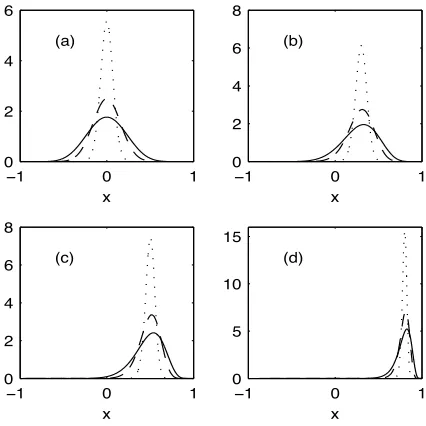
Fig. 2 shows the PDF of the rotary coefficient estimator for K= 10 and different values ofρandγ∗2.The PDF for negative
values of ρ is the reflection aroundx = 0 of the PDF for the corresponding absolute value. This can be seen from the fact that whenρ and x are simultaneously negated,yρx →1/yρx,
but (22) is invariant to such an inversion ofyρx,and (1−x2) in
(22) is invariant to a change in the sign ofx.
B. Confidence Intervals forρ(f)
Choose a fixed value of ρ. If we define points aα/2(ρ)
and a1−α/2(ρ) such that Fρˆ(aα/2(ρ);K, ρ, γ2∗) = α/2 and
Fρ(a1−α/2(ρ);K, ρ, γ∗2) = 1−α/2, whereFρˆ(x;K, ρ, γ∗2) is the
distribution function corresponding to the PDFfρˆ(x;K, ρ, γ∗2),
then
Pr[aα/2(ρ)≤ρˆ≤a1−α/2(ρ)] = 1−α. (23)
−1 0 1 0
2 4 6
(a)
x
−1 0 1
0 2 4 6 8
(b)
x
−1 0 1
0 2 4 6 8
(c)
x
−1 0 1
0 5 10 15
(d)
[image:5.595.58.271.59.272.2]x
Fig. 2. PDFfˆρ(x;K, ρ, γ∗2) forK = 10 and (a)ρ= 0 (b)ρ= 0.3 (c) ρ = 0.5 (d)ρ = 0.8 usingγ∗2 = 0,0.5,0.9,shown as solid, dashed and dotted lines, respectively.
−1 0 1
−1 −0.5 0 0.5 1
rotary coefficient
rotary coefficient estimate
(a)
−1 0 1
−1 −0.5 0 0.5 1
rotary coefficient (b)
Fig. 3. 95% confidence regions forρwhenγ∗2= 0.5 and (a)K= 10 and (b)K= 20.The dashed and dotted lines are explained in the text.
respectively, whenγ2
∗= 0.5.The dotted lines in Fig. 3(a) show
the interval (23) for a given value ofρ.
Confidence intervals forρare found by using the reverse strat-egy — see the dashed lines in Figs. 3(a) and (b). Given an es-timate ˆρ,here ˆρ= 0.7,we draw a horizontal dashed line across the plot at that value; the intersection of this line witha1−α/2 at ρ1 say, and with aα/2 at ρ2 say, defines a 95% confidence interval (α= 0.05) forρ as [ρ1, ρ2],which depends on the K used. The resulting 95% confidence intervals for ρ are [0.50, 0.83] forK= 10 and and [0.57, 0.80] forK= 20 when ˆρ= 0.7; as expected the interval is narrower with increasing number of complex degrees of freedomK.
Denote the 100(1−α)% confidence interval more fully by
[ρ1(ˆρ;α, K, γ∗2), ρ2(ˆρ;α, K, γ2∗)]. (24)
The interval is random since it depends on ˆρ, and it de-pends on the known quantities K and α, and the so-called ‘nuisance parameter’ γ2
∗. Computationally, given an estimate
ˆ
ρ of ρ, the right end of the interval, ρ2(ˆρ;α, K, γ2
∗), is the
value of ρ such that Fρˆ(ˆρ;K, ρ, γ∗2) −α/2 = 0, which can
be found simply using any standard zero-finding algorithm.
ρ1(ˆρ;α, K, γ∗2) is likewise found by finding the value of ρ for
−1 0 1
−1 −0.5 0 0.5 1
rotary coefficient
rotary coefficient estimate
(a)
−1 0 1
rotary coefficient (b)
Fig. 4. 95% confidence regions forρwhenK= 10 and (a)γ2
∗= 0.1 and
(b)γ∗2= 0.7.
whichFρˆ(ˆρ;K, ρ, γ∗2)−(1−α/2) = 0.As no analytical form for
Fρˆ(ˆρ;K, ρ, γ∗2) is forthcoming, it is necessary to calculate it by
[image:5.595.318.546.61.183.2]numerical integration of the PDF.
Fig. 4 shows the form of the 95% confidence regions for K = 10 and γ2
∗ values of 0.1 and 0.7. The region decreases
in size with increasing γ2
∗. So from Figs. 3 and 4 we see that
confidence intervals forρnarrow asKincreases, and also asγ2
∗
increases. The latter is explained by the fact that increasingγ2
∗
corresponds to increasingP2.
C. Simulated coverage intervals
The confidence interval (24) assumes knowledge ofγ2∗,but in
practice this will not be known. We carried out a simulation study to look at the coverage probability whenγ∗2 is first
esti-mated, then debiased, and then included in (24) in place of the unknown true value ofγ2
∗.
Three different matrices playing the role ofSU(f) in (3) were used in the simulations:
SU(1)=
5 −2 + 2i
−2−2i 2
; SU(2)=
10 7 + i
7−i 10
;
and
SU(3)=
2 1 + i
1−i 5
,
for whichρ= 0.43, γ2∗ = 0.8,for the first,ρ = 0, γ∗2 = 0.5,for
the second, and ρ =−0.43, γ∗2 = 0.2,for the third. For each
model matrix we simulated bivariate complex Gaussian vectors as in (17) using the method in [14, sec. V] and then combined them as in (11). K was chosen as 10 and 20. For each model matrix 5000 independent realizations of ˆSU were produced, and consequently 5000 realizations of ˆρfrom (12) and ˆγ∗2 from (14).
The estimates ˆγ∗2were debiased in two ways. Firstly an unbiased
estimate, ˜γ∗2,was obtained as
˜
γ∗2= 1−(1−ˆγ2∗)2F1(1,1;K; 1−ˆγ∗2), (25)
(e.g., [13, eqn. 24]), where2F1(a, b;c;y) is the hypergeometric function with 2 and 1 parameters and argument y. A second debiased estimate, ¯γ2∗,was found using the simpler formula [3]
¯
γ∗2= [Kγˆ2∗−1]/[K−1]. (26)
Since both these debiased estimates can be negative, they must be modified to max{0,˜γ2
∗}and max{0,γ¯∗2},respectively.
[image:5.595.54.283.330.452.2] [image:5.595.328.538.434.496.2]K Level M odel Conj. coherence
γ2
∗ ˜γ∗2 γ¯2∗
10 90% 1 90.1 88.3 89.8
2 89.9 88.4 89.3
3 89.5 88.8 89.1
95% 1 95.2 94.6 95.4
2 95.3 94.4 95.0
3 95.3 94.8 95.0
20 90% 1 90.3 89.9 90.5
2 90.1 89.3 89.6
3 90.4 89.9 90.1
95% 1 95.1 94.9 95.3
2 94.7 94.6 94.8
[image:6.595.311.552.59.258.2]3 95.1 95.2 95.3
TABLE I
Percentage of simulated random intervals containingρwhen
conjugate coherence is known or estimated.
−0.02 0 0.02
bias
(a) (b)
−1 0 1
0 0.02 0.04 0.06
rotary coefficient
mean squared error
(c)
−1 0 1
[image:6.595.56.280.64.244.2]rotary coefficient (d)
Fig. 5. Bias and mean squared errors (MSE). (a) bias whenγ2
∗ = 0.1,
(b) bias when γ∗2 = 0.7,(c) MSE whenγ∗2 = 0.1,and (d) MSE when γ2∗= 0.7.Solid lines are forK= 10 and dashed lines forK= 20.
The fact that we get close to nominal coverage when the con-jugate coherence nuisance parameter is not known but rather is estimated and debiased is the key to making the calculation of confidence intervals for the rotary coefficient of great practi-cal utility in the many scientific studies in which it is routinely used.
D. Bias and mean squared error
Two important properties of ˆρ, namely the bias,E{ρ} −ˆ ρ, and the mean squared error (MSE),E{(ˆρ−ρ)2}(variance plus squared bias), are shown in Fig. 5. Values were readily com-puted from moments derived from (22) using numerical integra-tion. We see that bias is positive for negative values of ρand
vice versa. Mean squared error is symmetric inρ,and largest at ρ= 0.Both bias and MSE decrease with increasingK and increasingγ2
∗.
IV. Data Analysis
Our example in the Introduction made use of ocean current speed and direction time series for one depth from a set of six
0
1000
2000
3000
4000
depth (m)
(a) (a) (a) (a) (a)
(a) (b)(b)(b)(b)(b)(b)
−1 −0.5 0 0.5
0
1000
2000
3000
4000
depth (m)
rotary coefficient (c) (c) (c) (c) (c) (c)
−1 −0.5 0 0.5
[image:6.595.53.283.291.470.2]rotary coefficient (d) (d) (d) (d) (d) (d)
Fig. 6. Estimated rotary coefficient (solid dot) and corresponding 95% confidence intervals (solid horizontal bars) for the six observation depths at the frequencies (c/hr) (a) 0.0518,(b) 0.0697,(c) 0.0911 and (d) 0.1095. Dotted lines delineate estimated change with depth.
(110, 760, 1260, 1760, 2510 and 3476m) recorded at a mooring in the Labrador Sea [10], [11]. We usedN= 1600 observations with a sampling interval of ∆t = 1hr. In the spectral analysis K= 10 sine tapers were applied. In this section we shall show the utility of the statistical results in this correspondence in providing insights into the nature of the ocean data. SinceWN
in (18) is 0.0034c/hr, the validity range WN ≤ |f| ≤ fN − WN for our statistical results for a finite-N sample is given by
0.0034≤ |f| ≤0.4966,hardly different to the asymptotic range 0<|f|<0.5.
Of great interest to oceanographers are deep ocean motions well away from boundaries, especially in the internal wave fre-quency band between about 10−2and 1c/hr. Fig. 1 covers this band, fairly central to which is the semi-diurnal tidal frequency (dashed). At a slightly lower frequency than the main tide will be the local inertial frequency which is latitude dependent.
Fig. 6 shows the estimated rotary coefficient (solid dot) and corresponding 95% confidence intervals (solid horizontal bars) for the six observation depths at the frequencies (c/hr) (a) 0.0518, (b) 0.0697, (c) 0.0911 and (d) 0.1095. These are the frequencies marked by the dotted lines in Fig. 1(b).
Starting with Fig. 6(b) atf= 0.0697c/hr, we see firstly that here the rotary coefficient is very close to−1 at all depths, (the confidence intervals are very narrow). This is what would be expected as anidealtheoretical outcome at the local inertial fre-quency, which is thus identified, suggesting that the statistical methodology has performed impressively well. At the frequency f= 0.0911c/hr, slightly higher than the tidal frequency, the ro-tary coefficient is more uncertain, Fig. 6(c), but does not appear to deviate greatly from about−0.8.For the lowest and highest of the four frequencies, Figs. 6(a) and (d) the most notable feature is the large deviations towards 0 at shallow depths.
−1 −0.5 0 0.5 1
rotary coefficient
(a)
0.02 0.04 0.06 0.08 0.1 0.12 0.14
−1 −0.5 0 0.5 1
rotary coefficient
freq (c/hr)
[image:7.595.48.286.60.257.2](b)
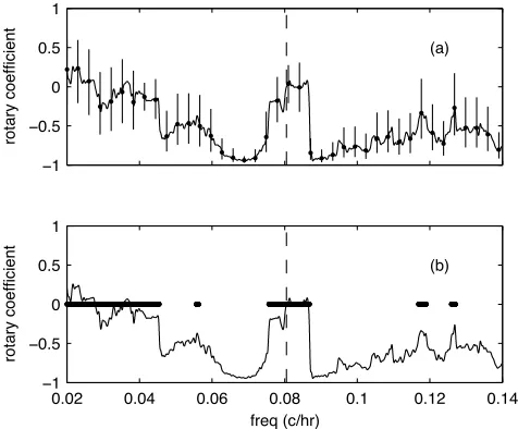
Fig. 7. Variation of estimated rotary coefficient as a function of frequency at depth 760m. (a) showing 95% confidence intervals (solid vertical bars) at a regular frequency spacing, (b) showing the frequencies at which the null hypothesis of rectilinear flow is not rejected (heavy bars). The semi-diurnal tidal frequency is shown by the vertical dashed line.
is not rejected at the 5% level. (The statistic (8) was used with distribution (9).) We see that these results are entirely consistent with the confidence intervals in Fig. 7(a); where the confidence interval includes zero the rectilinear flow hypothesis is not rejected, andvice versa.
V. Concluding comments
We have derived the basic statistical properties for the esti-mated rotary coefficient. These depend on the true value of the rotary coefficient, and the conjugate coherence γ∗2, a nuisance
parameter. Fortunately when the latter is estimated and debi-ased constructed confidence intervals maintain appropriate cov-erage probabilities, so such confidence intervals have practical utility as illustrated by the Labrador Sea current data analysis.
Acknowledgement
The authors are very grateful to Jon Lilly for making the Labrador Sea data available to them. Helpful comments and observations by the reviewers were much appreciated.
References
[1] H. H. Andersen, M. Højbjerre, D. Sørensen and P. S. Eriksen,Linear and Graphical Models. New York: Springer-Verlag, 1995.
[2] C. E. Barton, “Analysis of palaeomagnetic time series – techniques and applications,”Surveys in Geophysics, vol. 5, pp. 335-68, 1983
[3] V. A. Benignus, “Estimation of the coherence spectrum and its confidence interval using the fast Fourier transform,”IEEE Trans. Audio and Electroac.
vol. 17, pp. 145–50, 1969.
[4] D. R. Brillinger,Time Series: Data Analysis and Theory (Expanded Edition). New York: McGraw-Hill Inc., 1981.
[5] E. M. Carter, C. G. Khatri and M. S. Srivastava, “Nonnull distribution of likelihood ratio criterion for reality of covariance matrix,”J. Multivariate Analysis, vol. 6, pp. 176–84, 1976.
[6] W. J. Emery and R. E. Thomson,Data Analysis Methods in Physical Oceanog-raphy. New York: Pergamon, 1998.
[7] J. Gonella, “A rotary component method for analysing meteorological and oceanographic vector time series,”Deep-Sea Research, vol. 19, pp. 833-846, 1972.
[8] I. S. Gradshteyn and I. M. Ryzhik,Table of Integrals, Series, and Products (Corrected and Enlarged Edition). New York: Academic Press, 1980. [9] Y. Hayashi, “Space-time spectral analysis of rotary vector series,”J. of the
Atmospheric Sciences, vol. 36, pp. 757-66, 1979.
[10] J. M. Lilly, P. B. Rhines, M. Visbeck, R. Davis, J. R. Lazier, F. Schott and D. Farmer, “Observing deep convection in the Labrador Sea during winter 1994/95,”J. Phys. Oceanogr.,vol. 29, 2065–98, 1999.
[11] J. M. Lilly and P. B. Rhines, “Coherent eddies in the Labrador Sea ob-served from a mooring,”J. Phys. Oceanogr.,vol. 32, 585–98, 2002. [12] T. Maitani, “Statistics of wind direction fluctuations in the surface layer
over plant canopies,”Boundary-Layer Meteorology, vol. 26, 15–24, 1983. [13] T. Medkour and A. T. Walden, “Attenuation estimation from correlated
sequences,”IEEE Trans. Signal Process., vol. 55, pp. 378–83, 2007. [14] T. Medkour and A. T. Walden, “A variance equality test for two correlated
complex Gaussian variables with application to spectral power comparison,”
IEEE Trans. Signal Process., vol. 55, pp. 881–8, 2007.
[15] T. Medkour and A. T. Walden, “Statistical properties of the estimated degree of polarization,” IEEE Trans. Signal Process., vol. 56, pp. 408–14, 2008.
[16] K. S. Miller, Hypothesis Testing with Complex Distributions. New York: Robert E. Krieger, 1980.
[17] C. N. K, Mooers, “A technique for the cross spectrum analysis of pairs of complex-valued time series, with emphasis on properties of polarized com-ponents and rotational invariants,”Deep-Sea Research, vol. 20, pp. 1129–41, 1973.
[18] I. Olkin and J. W. Pratt, “Unbiased estimation of certain correlation co-efficients,”Annals of Mathematical Statistics, vol. 21, pp. 201–211, 1958. [19] M. Orli´c, B. Penzar, and I. Penzar, “Adriatic sea and land breezes:
clock-wise versus anticlockclock-wise rotation,”J. Appl. Meteorology, vol. 27, pp. 675–9, 1988.
[20] D. B. Percival and A. T. Walden,Spectral Analysis for Physical Applications. Cambridge, UK: Cambridge University Press, 1993.
[21] M. S. S. Sarma, and L. V. Gangadhara Rao, “Spectra of currents and temperature off Godavari (East Coast of India),”Mahasagar, vol. 22, pp. 29-36, 1989.
[22] B. Picinbono and P. Bondon, “Second-order statistics of complex signals,”
IEEE Trans. Signal Processing, vol. 45, pp. 411–420, 1997.
[23] P. J. Schreier, “Polarization ellipse analysis of nonstationary random sig-nals,”IEEE Trans. Signal Processing, vol. 56, pp. 4330–4339, 2008. [24] P. J. Schreier and L. L. Scharf, “Second-order analysis of improper
com-plex random vectors and processes,”IEEE Trans. Signal Processing, vol. 51, pp. 714–725, 2003.
[25] P. J. Schreier and L. L. Scharf,Statistical Signal Processing of Complex-Valued Data. Cambridge, UK: Cambridge University Press, 2010. [26] H. van Haren and C. Millot, “Rectilinear and circular inertial motions
in the Western Mediterranean Sea,” Deep-Sea Research Part I, vol. 51, pp. 1441–55, 2004.
[27] A. T. Walden, E. J. McCoy and D. B. Percival, “The variance of multi-taper spectrum estimates for real Gaussian processes,”IEEE Trans. Signal Processing, vol. 42, pp. 479–482, 1994.
[28] A. T. Walden, E. J. McCoy and D. B. Percival, “The effective bandwidth of a multitaper spectral estimator,”Biometrika, vol. 82, 201–214, 1995. [29] L. Zhiliang, H. Dunxin, T. Xiaohui, and W. Enbo, “Rotary spectrum