COMPARISON OF JAMMING EXCISION METHODS FOR DIRECT SEQUENCE/SPREAD SPECTRUM (DS/SS) MODULATED SIGNAL

MODIFIED VIRTUAL FORCE METHOD FOR MOBILE

ROBOT NAVIGATION

1

MENDILI MANEL, 2BOUANI FAOUZI

1, 2

Universite De Tunis El Manar, Ecole Nationale D’ingenieurs De Tunis

Lr11es20, Laboratoire D’analyse, Conception Et Commande Des Systemes, Tunis, Tunisie. E-mail: [email protected], [email protected]

ABSTRACT

This paper deals with the problem of target tracking of two wheeled mobile robots with obstacle avoidance. The model predictive control approach and the virtual force method are used to compute the control sequence applied to the mobile robot. The force is proportional with the distance between the robot and the obstacle. Simulations are performed and their results are provided to show the effectiveness of the proposed method. This paper improves the formulae of force computing in the virtual force method to avoid the obstacles.

Keywords: Two Wheeled Mobile Robot, Predictive Control, Obstacle Avoidance, Virtual Force

1. INTRODUCTION

In challenging environments, the robot needs to gather information about their surroundings to avoid obstacles for outer space exploring robots this is more important because there can be a belay of between control station and the robot. Nowadays, even in ordinary environments detecting and avoiding obstacles are required. Thus obstacle avoidance function is a primary requirement of any autonomous mobile robot, starting with primitive algorithms that detect an obstacle and stop the robot in order to avoid it, passing to the more complex algorithms involving detection of obstacles as a measurement concerning the obstacle dimension to allow the algorithm to steer the robot around the obstacle.

During the past few years, potential field methods for obstacle avoidance have been the subject of many researches. The idea of imaginary forces acting on a robot has been suggested by Andrews and Hogan and Khatib, in these approaches obstacles exert repulsive forces onto the robot, while the target applies an attractive force. The sum of all forces determines the direction and speed of the robot. It is a simple and reliable method. Thus in this paper we have chosen to work on this method and ameliorate its capacities to steer the robot around the obstacle.

2. RELATED WORKS

Obstacle avoidance is a key issue to acknowledged applications of mobile robot because collisions with

any item cause an unsuccessful mission; this makes the obstacle avoidance for mobile robot an object of many researches.

Researchers have concentrated more on the applications of autonomous mobile robots. Nevertheless, obstacle avoidance for non autonomous mobile robot is particularly important. The more commonly employed technique is based on edge detection. The algorithm of this method determines the vertical edges of the obstacle and tries to conduct the robot around these edges, the line connecting the edges is considered as an obstacle boundary. This technique is used in many works [1], [2]. Another generally used method is certainty grid for obstacle representation. This method has been developed in [3]. The robot's area is represented by two dimensional arrays of square elements denoted cells. The confidence of the obstacle existence is indicated by a certainty value which is updated taking into account the characteristics of the sensor. The disadvantage of this method is on edge detecting; the robot is needed to stop in front obstacle then moves to another location.

follows the desired trajectory and avoids collision with obstacles while trying to match the prescribed trajectory as closely as possible [6], [7].

Many control laws have been used for the problem of trajectory tracking; however the model predictive control is a control approach that overcomes the limits of other classical techniques since the control sequence is simply calculated by minimizing a cost function obtained through the prediction of the output system over a predefined horizon in order to control variables and to make the controlled variables as close as possible to reference trajectories [8].

Even though model predictive control is an ancient control method, works dealing with model predictive control and wheeled mobile robots are scarce. Nonlinear model predictive control techniques have been proposed in the literature [9], [10] but we should know that the computational effort necessary in this case is much higher than the linear version. We should also know that in nonlinear predictive control there is a nonlinear programming problem which is solved online [11]; it is non convex and it has a big number of decision variables so that a global minimum is in general difficult to find. Linearization is proposed to overcome the problems related to the nonlinear method [12].

In previous works, we presented the model predictive control solving the problem of trajectory-tracking of two wheeled mobile robot [13]. As continuation, we work in this paper on the problem of obstacle avoidance using the repulsive force.

3. PREDICTIVE CONTROL OF TWO WHEELED MOBILE ROBOT

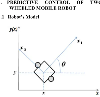
[image:2.612.94.295.491.685.2]

2.1 Robot’s Model

Figure 1. The Scheme Of Two Wheeled Mobile Robot

Generally, to control a mobile robot we use a kinematic model instead of a dynamic one because calculating the control law is then easier and there are no complicated geometric parameters. Considering the following simplifying hypotheses:

The mobile robot is regarded as a rigid vehicle moving in horizontal plane.

The conventional wheels are assumed dimensionally stable.

Each contact wheel/ground is reduced to a point; wheels roll without sliding on the ground.

Considering the mobile robot in figure 1 the kinematic model is then given as follows [13], [14]:

cos 0

sin 0

0 1

x

v y

θ θ

ω θ

   

 

  ₌ 

 

   _{  }

   

   

& & &

(1)

where v and ω denote respectively, the linear velocity and the angular velocity and they are regrouped in a vectorU=

[

v ω

]

T.

In model predictive control a model is used and the control law is calculated in discrete-time, consequently we present a discrete -time model with a sampling period Ts and a sampling instant k.

Using Euler's approximation relation (1) gives.

( 1) ( ) ( ) cos ( ) ( 1) ( ) ( ) sin ( )

( 1) ( ) ( )

s

s

s

x k x k T v k k

y k y k T v k k

k k T k

θ θ

θ θ ω

+ = +



 _{+ = +}



 _{+ = +}



(2)

We note by Xref the pre-known reference

trajectory and we associate generally to this reference trajectory a virtual robot having the same model of the controlled one.

2.2Predictive Control Approach

The problem of trajectory tracking is stated as to find a control law to obtain

X k( )−Xref( )k 0 (3)

where

( ) ( ) ( ) ( ) x k

X k y k

k θ

 

 

=  

 

 

and

( )

( ) ( )

( )

ref

ref ref

ref

x k

X k y k

k θ

 

 

=  

 

 

time in a QP problem. Writing (2) around Xref

gives us the following formulae:

( 1) ( ) ( ) cos ( )

( 1) ( ) ( ) sin ( )

( 1) ( ) ( )

ref ref s ref ref

ref ref s ref ref

ref ref s ref

x k x k T v k k

y k y k T v k k

k k T k

θ θ

θ θ ω

 + = +  _{+ = +}   _{+ = +}  (4)

We linearize the system model by computing an error model with respect to a reference trajectory and we expand the kinematic model in Taylor series around the point

(

Xref,Uref

)

,

at each sampling time k we obtain these formulae:

cos ( ) ( ) sin ( )cos

sin ( ) ( ) cos ( )sin

( ) ( )

ref s ref ref ref s ref ref ref s ref ref

ref s ref ref ref s ref ref ref s ref ref

ref ref s ref s ref

x Tv x x T v T v v y Tv y y T v T v v

T T

θ θ θ θ θ

θ θ θ θ θ

θ ω θ θ ω ω

 + + − − − + −  _{+ + − − − + −}   _{+ + − + −}  (5)

We obtain the discrete-time model of the system by using (4) and (5).

X k%( + =1) A k X k( ) ( )% +B k U k( ) ( )% (6)

With

1 0 ( ) sin ( ) ( ) 0 1 ( ) cos ( )

0 0 1

cos ( ) 0 ( ) sin ( ) 0

0

s ref ref

s ref ref

s ref

s ref

s

T v k k

A k T v k k

T k

B k T k

T θ θ θ θ −     =           =       (7)

where X k%( )=X k( )−Xref( )k represents the error with respect to the reference car and

ref

U% =U−U is its associated error control input.

The linearization around a stationary operating point makes the robot non controllable because the robot is not moving so it cannot be steered from an initial state to a final state by using finite inputs. Nevertheless, U is not zero which makes the linearization becomes controllable and the tracking of a reference trajectory is possible with the linearized model predictive control.

Let's introduce these vectors:

( 1/ ) ( )

( 2/ ) ( 1)

( 1) . U(k) = .

. .

( / ) ( 1)

X k k U k

X k k U k

X k

X k N k U k N

 +        + +         + =          ₊   _{+ −}      % % % % % % (8)

where N is the prediction horizon. With the weighting matrices Q for the error in the state and R for the control variables we can write the objective function to be minimized as follows.

1 1

( ) ( / ) ( ) ( / ) ( 1) ( ) ( 1)

N N

T T

j j

k X k j k Q j X k j k U k j R j Uk j φ

= =

=

∑

% + % + +

∑

% + − % + − ₍₉₎

Introducing the vectors in (8) with the function (9) allows us to write the cost function: ( )k XT(k 1) (Q X k 1) UT( )k RU k( )

φ = + + + (10)

whereQ=diag Q( ),R=diag R( ).

We deduct from (6) and (8) a new state model of robot's system:

X k( + =1) A k X k( ) ( )% +B k U k( ) ( ). (11)

Aand Band ( , , )β k j l are given by:

1

( , , ) ( / )

i N j

k j l A k i k

β

= −

=

∏

+ (12)

( / ) ( 1 / ) ( / )

. . . ( , 2, 0)

( ,1, 0)

A k k

A k k A k k

A k k β β    ₊        =             (13)

( ) 0 . . . 0

( 1) ( ) ( 1) . . . 0

. . . .

. . . .

. . . .

( ,2,1) ( ) ( ,2,2) ( 1) . . . 0 ( ,1,1) ( ) ( ,1,2) ( 1) . . . ( 1) B

Bk

Ak Bk Bk

k Bk k Bk

k Bk k Bk Bk N

β β β β =    _{+ +}              +    _{+ + −}    (14)

( ) ( ) ( ) ( ) ( ) ( ) + ( )

( ) 2( )

( ) 2 ( / )

( ) ( / ) ( / )

T T

T

T

T T

k U k H k U k f k U k d k where

H k B Q B R

f k B Q AX k k

d k X k k A Q AX k k

φ = +

= +

=

=

%

% %

(15)

We note that d is independent of U and has no influence in the determination of the optimal input thus (15) turns to a standard expression used in QP problems and the o8ptimization problem to be solved at each sampling time.

4. OBSTACLE AVOIDANCE

4.1 Principle of ultrasonic detection

The two wheeled mobile robot uses ultrasonic sensors for its movements and a microcontroller is used to achieve the desired operation. The ultrasonic sensor is attached in front of the robot. Whenever the robot is going on the desired path the ultrasonic sensor transmits the ultrasonic waves continuously from its sensor head. Whenever an obstacle comes ahead of it the ultrasonic waves are reflected back from an object and that information is passed to the controller device to regulate the speed of the robot.

The ultrasonic sensor emits a signal that propagates in the air at the velocity of sound as shown in figure 2. If it hits any object, then it reflects back an echo signal to the sensor. The ultrasonic sensor is composed of a multi vibrator, fixed to the base. The multi vibrator contains a resonator and a vibrator. The resonator delivers ultrasonic waves generated by the vibration. The ultrasonic sensor then consists of two parts; the emitter and the detector. So that the ultrasonic sensor enables the robot to virtually see object, measure distance and avoid obstacles.

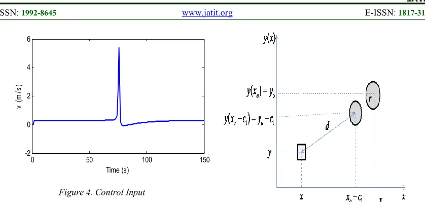
[image:4.612.328.525.472.656.2]

The role of the ultrasonic sensor in the next section is allowing us to detect the coordinates of the obstacle

(

x y_o, _o

)

.

Figure 2. Ultrasonic Working Principle

4.2 Virtual Force Obstacle Avoidance

The ultrasonic sensor detects the obstacle from a specified distance so when the obstacle is detected the robot produces a repulsive force which is inversely proportional to the distance between the obstacle and the robot [5].

Classical method of virtual force obstacle avoidance

• Problem stating

The distance between the obstacle and the robot at each sampling time is computed as follows:

( )² ( )²

ro o o

d = x−x + y−y (16)

(

x yo, o

)

is the position of the center of the obstacle.

(

x y,

)

is the position of the robot at each sampling time.

The repulsive force pushing the robot away from the obstacle is inversely proportional to the square of the distance between the obstacle and the robot and their two terms are defined as follows:

2

2 o r

x

ro ro

o r

y

ro ro

x x F UF

d d

y y F

UF

d d

 − 

= _{ }

 

 − 

= _{ }

 

(17)

where Fris a force constant chosen by the user.

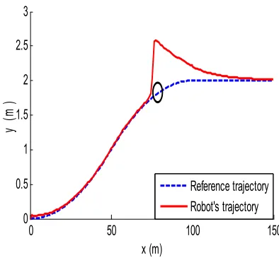
0 50 100 150

0 0.5 1 1.5 2 2.5 3

x (m)

y

(

m

)

Reference trajectory Robot's trajectory

[image:4.612.103.292.651.711.2]

0 50 100 150 -2

0 2 4 6

Time (s)

v

(

m

/s

[image:5.612.94.513.66.265.2]

)

Figure 4. Control Input

Figure 3 shows that using the method of virtual force to avoid the obstacle the robot reaches the obstacle than it goes far from the obstacle and we note also that it goes so far away that it takes long time to reach the reference trajectory again so we propose some modification in the formulae of the method of virtual force to allow the robot to avoid the obstacle before reaching it and to decrease the amplitude of the trajectory taken by the robot to avoid the obstacle. Figure 4 shows the variation of the control input.

• Chosen solution

To allow the robot avoid the obstacle before reaching it we though to introduce a constant in the computing of the distance between the robot and the obstacle this constant c1 is introduced in (18) with the obstacle abscise and ordinate.

And to allow the robot goes smoothly around the obstacle we varied the exponent of d to a a rational number.

Modified method of virtual force obstacle avoidance

The distance between the obstacle and the robot at each sampling time is computed by the use of the figure 5. Figure 5 defines the distance between the robot and the obstacle which is calculated with this formula:

1 1

( ( ))² ( ( ))²

ro o o

d = x− x −c + y− y −c (18)

c1is a constant value chosen by the user to avoid

the obstacle before reaching it; c1 would include the

obstacle radius value if it is known.

yo-c1 isthe corresponding ordinateto (xo-c1) in the

reference trajectory.

Figure 5. The Distance Between The Robot And The Obstacle

The forces are calculated with the following formulae:

1 3

2

1 3

2

( )

( )

o r

x

ro ro

o r

y

ro ro

x x c F

UF

d d

y y c F

UF

d d

 − − 

= _{ }

 

 − − 

= _{ }

 

(19)

The force constant is divided by

3 2 ro

d . By this method, the robot exerts strong repulsive forces when it is in the immediate vicinity of the obstacles, and weak forces when they are further

away. Notice that in (19) the use of 3

2minimizes the strength of the repulsive force so that the robot does not go so far away from the trajectory.

The control input applied to each robot includes two terms [6]; one to keep the robot tracking the desired trajectory and another to avoid the obstacles.

( ) ( ) ( )

0

T

v UF

U k U k UF k

ω

   

= + =_{  }+ _

    (20)

where 2 2

x y

UF= UF +UF and it is added to the linear velocity which means the first component of U _.

5. SIMULATION

The aims of the simulations are to examine the effectiveness and performance of the predictive controller based on the p kinematic model of two wheeled mobile robot with the virtual force method to avoid the obstacles.

We compared the results of avoiding obstacles using the classical virtual force method and the modified one. And to show the effectiveness of our modifications we took the case of one obstacle , two obstacles, different radius of obstacle and different values of repelling force.

• Simulation results

We simulate the model predictive control and the obstacle avoidance approach to show the effectiveness of the proposed method of two wheeled robot control using MATLAB and we compare the performances of the modified virtual force method with the classical one. We consider N= 20, Ts= 0.1s, R= Q= I.

The reference trajectory is considered as follows:

²

0 50 2500

( 100)²

( ) 2 50 100

2500

2 100 150

r

r

r

r r r

r

x

x

x

y x x

x

 _{≤ <}

 

− −



= + ≤ <



≤ < 

 

(21)

We have considered the constant c1=5m and the

robot's radius is chosen r = 0.5m.

The robot starts from the initial point (0, 0) and updates its control law at each sampling time. The reference trajectory is tracked then the robot meets the obstacle and deals with it.

It is shown by the simulation in figure 6 that the control law joined with the technique of virtual force has allowed the robot to avoid the obstacle; the robot kept a safe distance from the obstacle and after a short time the robot met the desired trajectory.

0 50 100 150

0 0.5 1 1.5 2 2.5 3

x (m)

y

(

m

)

[image:6.612.322.520.81.260.2]

Reference trajectory classical method modified method

Figure 6. Robot's Obstacle Avoidance At (75,1.75)

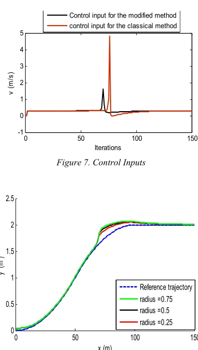
0 50 100 150

-1 0 1 2 3 4 5

Iterations

v

(

m

/s

)

[image:6.612.317.514.275.623.2]

Control input for the modified method control input for the classical method

Figure 7. Control Inputs

0 50 100 150 0

0.5 1 1.5 2 2.5

x (m)

y

(

m

)

Reference trajectory radius =0.75 radius =0.5 radius =0.25

0 50 100 150 0

0.5 1 1.5 2

Time (s)

v

(

m

/s

)

[image:7.612.160.514.53.615.2]

radius =0.25 radius =0.5 radius =0.75

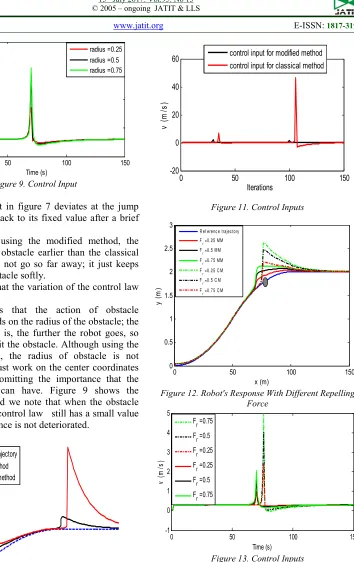
Figure 9. Control Input

The control input in figure 7 deviates at the jump point and turns back to its fixed value after a brief time.

We notice that using the modified method, the robot avoids the obstacle earlier than the classical method and does not go so far away; it just keeps safe from the obstacle softly.

We also notice that the variation of the control law is smaller.

Figure 8 shows that the action of obstacle avoidance depends on the radius of the obstacle; the bigger the radius is, the further the robot goes, so that it does not hit the obstacle. Although using the classical method, the radius of obstacle is not considered; we just work on the center coordinates of the obstacle omitting the importance that the obstacle radius can have. Figure 9 shows the control inputs and we note that when the obstacle radius is 0.75m, control law still has a small value and the performance is not deteriorated.

0 50 100 150 0

1 2 3 4 5 6

x (m)

y

(

m

)

Reference trajectory Modified method Classical mmethod

Figure 10. Robot's Obstacle Avoidance At (35, 0.49) And (105,2)

0 50 100 150 -20

0 20 40 60

Iterations

v

(

m

/s

)

[image:7.612.314.518.121.609.2]

control input for modified method control input for classical method

Figure 11. Control Inputs

0 50 100 150

0 0.5 1 1.5 2 2.5 3

x (m)

y

(

m

)

R e f e re nc e trajec to ry F

r =0 .2 5 MM

F

r =0 .5 M M

F

r =0 .7 5 MM

F

r =0 .2 5 C M

F

r =0 .5 C M

F

r =0 .7 5 C M

Figure 12. Robot's Response With Different Repelling Force

0 50 100 150

-1 0 1 2 3 4 5

Time (s)

v

(

m

/s

)

F_r =0.75

F_r =0.5

F_r =0.25

F_r =0.25

F_r =0.5

F_r =0.75

Figure 13. Control Inputs

[image:7.612.92.294.498.668.2]

.

Figure 12 illustrates the fact that the more the value of force is elevated, the more the robot goes far from the obstacle. The best value verified here is Fr

= 0.25 to let the robot avert the obstacle softly. Figure 13 shows the different control laws for the different force constants using the classical and the modified method.

The different studied cases have proved the effectiveness of the modifications introduced to the method of computing the virtual force applied to the robot. The robot then avoids the obstacle smoothly and before reaching it. These are our goals that we tried to ameliorate in the classical virtual force method of avoiding obstacles.

• Future works

We have introduced here a kinematic model and developed a control system with high performances and our perspectives are to continue the experimental implementation and to compare the virtual force method with other methods of avoiding obstacle to ameliorate the results.

6. CONCLUSIONS

This paper presents the model predictive control joined with the virtual force obstacle avoidance to allow the robot track the reference trajectory and avert any obstacle to complete its mission. Simulations showed that the modification done on the virtual force formulae made it more effective, unwrinkled and reliable. The proposed approach makes the robot then avoid more than one obstacle, obstacles with different radius even if we vary the value of the repelling force.

REFERENCES

[1] J.L; Crowley. “ Dynamic world modeling for an intelligent mobile robot using a rotating ultra-sonic ranging device”. IEEE International Conference on Robotics and Automation, March 25-28, St. Louis 1985.

[2] Kuc.R; Barshan. B. “Navigating vehicles through an unstructured environment with sonar”, IEEE International Conference on Robotics and Automation, Vol. 3, Scottsdale, AZ, pp. 1422–1426, 1989.

[3] A.Elfes. “Sonar-Based Real World Mapping and Navigation”,IEEE J.Robotics and Automation, Vol. RA-3, No. 3, June 1987

[4] Khatib. O. “Real-Time Obstacle Avoidance for Manipulators and Mobile Robots”, IEEE International Conference on Robotics and Automation, March 25-28, St. Louis, pp. 500-505, 1985.

[5] Borenstein. J , Koren. Y. “Tele-autonomous Guidance for Mobile Robots”, IEEE Transactions on Systems, Man, and Cybernetics, special issue on unmanned systems and vehicles, pp. 1437-1443, December 1990.

[6] Borenstein J. , Koren. Y. “Real-time Obstacle Avoidance for Fast Mobile Robots in Cluttered Environments”, IEEE International Conference on Robotics and Automation, Cincinnati, Ohio, pp. 572-577, May 13-18, 1990.

[7] A.Mohammadi, M. Bagher Menhaj, A.Doustmohammadi. “Distributed Model Predictive Control and Virtual Force Obstacle Avoidance for Formation of Nonholonomic Agents”, 2nd International Conference on Control, Instrumentation and Automation (ICCIA) , pp. 440-445, 2011.

[8] H. Salhi , F. Bouani ; M. Ksouri. “Constrained MIMO Nonlinear Predictive Control based Derivate-free state estimators” International Conference on Control, Decision and Information Technologies (CoDIT), Hammamet, Tunisia, May 2013.

[9] A.Khalaji, M.Bidgol, S.Moosavian. “Non-model-based control for a wheeled mobile robot towing two trailers”, Proceedings of the Institution of Mechanical Engineers, Part K: Journal of Multi-body Dynamics, September 2014.

[10] C.Hsieh, J. Liu. “Nonlinear Model Predictive Control for Wheeled Mobile Robot in Dynamic Environment”, The IEEE/ASME International Conference on Advanced Intelligent Mechatronics, Kaohsiung, Taiwan, July 11-14, 2012.

[11] H. Lim, Y. Kang, C. Kim, J. Kim, B. You. “Nonlinear Model Predictive Controller Design with Obstacle Avoidance for a Mobile Robot”, IEEE/ASME International Conference on Mechatronics and embedded systems and applications , Beijing, 12-15 Oct. 2008.

[12] G. Campion, G. Bastin, B. d’Andrea Novel. “Structural properties ´ and classification of kinematic and dynamic models of wheeled mobile robots”, IEEE Trans. on Robotics and Automation, vol. 12, no. 1, pp. 47–62, 1996. [13] M.Mendili, F.Bouani. “Trajectory tracking of

two wheeled mobile robot”, 6th International Conference on Modeling, Simulation and Applied Optimization, Istanbul, Turkey, may2015. [14] Kühne, F. Lages, W. Gomes da Silva; J .“Mobile