Yield Estimation for a Single Purpose Multi-Reservoir
System Using LP Based Yield Model
Deepak V. Pattewar1, Kalpeshkumar M. Sharma1, P. D. Dahe2 1Civil Engineering Department, M. G. M’s College of Engineering, Nanded, India. 2Civil Water Management, S. G. G. S College of Engineering and Technology, Nanded, India
Email: [email protected], [email protected]
Received April 17,2013; revised May 22, 2013; accepted July 1, 2013
Copyright © 2013 Deepak V. Pattewar et al. This is an open access article distributed under the Creative Commons Attribution Li-cense, which permits unrestricted use, distribution, and reproduction in any medium, provided the original work is properly cited.
ABSTRACT
Application of optimization techniques for determining the optimal operation policy for reservoir is a major area in wa-ter resources planning and management. Linear programming, ruled by evolution techniques, has become popular for solving optimization problems in diversified fields of science. An LP-based yield model (YM) has been used to re-evaluate the annual yield available from the reservoirs for irrigation. This paper extends the basic yield model and pre-sents a yield model for a multiple-reservoir system consisting of single-purpose reservoirs. Optimum yield of reservoirs system is calculated by yield model. The objective is to achieve prespecified reliability for irrigation and to incorporate an allowable deficit in the annual irrigation target. The yield model is applied to a system of two reservoirs in the Manar River in India. This model can act as a better screening tool in planning by providing outputs that can be very useful in improving the efficiency and accuracy of detailed analysis methods such as simulation.
Keywords: Yield Model; Reservoir Operation; Irrigation Releases; Manar River
1. Introduction
Linear Programming (LP) is a commonly used optimiza-tion approach in water resources management. It is con-cerned with solving a special type of problem; one in which all relations among the variables are linear, both in constraints and the objective function to be optimized. An application of LP to reservoir operations has varied from simple straightforward allocation of resources to complex situations of operation and management. In the past, limitations of computing power meant that optimi-zation was achieved by decomposing reservoir systems in time and space. These early models were predomi-nantly deterministic, that is, they did not take into ac-count the stochastic nature of inflows but rather were based on long-term average seasonal or monthly flows. However, they have gradually been improved. For ex-ample, Loucks [1] developed a stochastic LP technique for a single reservoir subject to random, serially corre-lated, flows. Subsequently, much more complicated sto-chastic models have been developed to reflect more real-istically stream flow stochasticity, evaporation losses and more complex systems involving multiple reservoirs (Dandy G.C., Connarty M.C and Locks D.P. [2]; William
W. G. Yeh [3]). Under certain assumptions, non-linear
This study presents a methodology to optimize the de-sign of the multi-reservoir irrigation system by taking monthly inflow and initial storage and tries to predict the maximum possible releases using Linear programming based Yield model. The specific objectives of the present study can be stated as fallows:
1) To develop a Linear Programming based yield mo- del for reservoir operation for a monthly time step.
2) Comparison of yield model and actual irrigation re-leases for single purpose irrigation reservoirs in Manar River.
3) To draw the conclusions from the interpretation of results obtained.
2. Reservoir Yield Model
The conceptualisation and details of the yield model on which the present model development is based are
pre-sented in Loucks et al. [8]. When reservoir yield with
reliability lower than the maximum reliability is to be determined, the extent of availability of yield (or the al-lowable deficit in yield) during failure years can be specified. This is achieved by specifying a failure frac-tion for the yield during the failure years. The factor θp,j
is used in the model to define the extent of available yield during failure years. The objective of this model is to maximize the yield for given capacity of the reservoir.
Let p denotes the exceedence probability for the yield.
The index j refers to a year and index t refers to a
within-year period. In this model only the firm yield is used.
The yield model given by Dahe and Srivastava [6] to determine single yield from a reservoir is as follows.
The formulation of the yield model is as follows: Objective function
Maximize
, ,
1f p 2f p
Oy Oy
o 1, 1,
(1)
Constraint
1) Over-year storage continuity
o ,
1, 1 1, 1, , 1,
f p
j j p j j j j
s I Oy Sp El s
o 1, 2,
(2)
o ,
2, 1 2, 2, , 2, 2,
f p
j j p j j j j j
s I Oy Sp El Sp s
, ,
1 2
(3) The over-the-year capacity is governed by the distri-bution of annual stream flows and the annual yield to be provided. The maximum of all the over-the-year storage volumes is the over-the-year storage capacity. It is possi-ble to specify a failure fraction to define the allowapossi-ble deficit in annual reservoir yield during the failure years in a single-yield problem. In the above equation,
f p f p
Oy Oy
o 1, 1
is the safe (firm) annual yield from Up-per Manar reservoir and Lower Manar reservoir with
o 1, and
reliability p. s j s j are the initial and the final
over-the-year active storages in year j for the Upper
Manar reservoir and similarly for the Lower Manar
o 2, 1
o 2, j
s and s j respectively; I1,j and I2,j
1,
are the
inflows in year j (Upper Manar and Lower Manar in
Manar River); θp,jis the failure fraction defining the
pro-portion of the annual yield from reservoir to be made available during the failure years to safeguard against the risk of extreme water shortage during the critical dry periods (θp,j lies between 0 and 1, i.e., for a complete
failure year θp,j =0, for a partial failure year 0 < θp,j <1,
and for a successful year θp,j =1); El j and El2,j 1,
= evaporation loss in year j and Sp j and Sp2,j
o 1, 1j 1
excess- release (spills) in year j;
2) Over-year active storage volume capacity
s Y
o 2, 1j 2
(4)
s Y
,
1, 1 1, 1 1, 1, , 1 1,
w f p t t w
t t t f p t
t
(5)
The active over-year reservoir capacity (Y1) required
for delivering a safe or firm annual yield in Upper Manar
reservoir and active over-year reservoir capacity (Y2)
required for delivering a safe or firm annual yield in Lower Manar reservoir
3) Within-year storage continuity
Oy El Oy El s
,2, 1 2, 2 2,
2, , 2 0.10 1, , 2,
w f p
t t t
t
t t t w
s (6)
f p f p t
s Oy El
Oy El Oy s
1, 1, 2, 1
w w
t t
(7)
Any distribution of the within-the-year yields differing from that of the within-the-year inflows may require ad-ditional active reservoir capacity. The maximum of all the within-the year storage volumes is the within-the-
s s
year storage capacity. In the above equation,
1,, 2, w w t t
and s s
1,t
are the initial and the final within-the-
year active storages at time t; and 2,t are the
ratio of the inflow in time t of the modelled critical year
of record to the total inflow in that year; and and
are the within-the-year evaporation losses during
1,t
El
2,t
El
time t. The inflows and the required releases are just in
balance. So, the reservoir neither fills nor empties during the critical year.
4) Definition of estimated evaporation losses (Over- year)
1, 1 1, 0
1, 1 1, 1 1, 1
1 0
2
w w
t t r
j j t
t
s s
E E s El
2, 1 0
2, 2 2, 1
2, 2,
1 0
2
w w
t t
j j t
t
s s
E E s
(9)
5) Definition of estimated evaporation losses (Within- year)
2 r
El
1, 1 1, o
1 1, 1 1, 1
1 0
2
t t
t r
t cr t
E E s El
(10)
w w
s s
2, 1 o
2 2, 2
1 0
2
t cr
E E s 2,
2, 2
w w
t t
t r
t
s s
El
6) Total reservoir capacity
1 1, 1wt 1
Y s Ya
2
Ya
(13)
Sum ear and the w
age capacities is equal to the active storage capacity of the reservoir.
(11)
(12)
2 2, 1 w
t
Y s
of the over-the-y ithin-the-year
stor-7) Proportioning of yield in within-year periods
,
1, , 1, 1
p t
f p t f
Oy K Oy (14)
,
2, , 2, 2
p t
f p t f
Oy K Oy (15)
1,t
K and K2,t defines a predete tio
l reservoir yield to be supplied in the with yield in period t.
The tions
, a tributary of Manjara River in Goda-anar River pper Manar rmined frac n of
an-nua in-year
Equa (1) to (15) present the Multi-reservoir
yield model for Upper Manar and Lower Manar reservoir in Manar River.
2.1. System Description: Manar River
The Manar River
vari basin, Maharashtra states in INDIA. In M
two medium project has constructed i.e. U
and Lower Manar reservoir for irrigation preposes
Fig-ure 1. Table 1 is the silent features of Upper Manar Pro-
1 2
1- Upper Manar
for Irrigation
Purpose
2-Lo
Irrigat
wer Manar for
ion Purpose
Manar river
Inflow
Evaporation Evaporation
[image:3.595.66.288.170.294.2]Spill Spill
Figure 1. Line diagram of reservoir system on Manar River.
ject Limboti reservoir and Lower Manar Project-Barul reservoir. A 37 years historic inflow data for the system considered is available as shown in Figures 2 and 3.
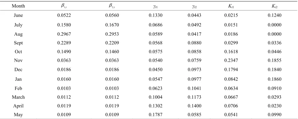
2.1.1. Irrigation Parameters (Kt) for Upper Manar
Limboti Reservoir and Lower Manar Barul Reservoir
The monthly proportions of the annual irrigation targets
(Kt values) are worked out by considering the cropping
patterns and irrigation intensities recommended by the
agricultural officer. Kt defines a predetermined fraction
of reservoir yield the within-year period t. The Kt value are given in Table 2.
[image:3.595.338.504.406.536.2]s
Figure 2. Inflow at Upper Manar-Limboti reservoir.
[image:3.595.61.288.580.716.2]Figure 3. Inflow at Lower Manar-Barul reservoir.
Table 1. Silent features of Upper Manar and Lower Manar project in Manar River.
Particulars Upper Manar Lower Manar
Irrigation Purpose Irrigation Purpose Scope of Scheme
Location Manar River at
Limboti Manar River at Barul Catchment area 987.60 Sq Km 1585.08 Sq Km Gross storage capacity 107.98 MCM 146.92 MCM
Capacity of Live
Storage 75.71 MCM 138.21 MCM
Capacity of
Dead Storage 32.27 MCM 8.71 MCM 75% dependable
[image:3.595.309.538.592.734.2]w approximation, irrigation and evaporati sed i odel fo Mana
[image:4.595.57.539.111.304.2]Month
Table 2. Within-year inflo on parameters u n the yield m r reservoirs on
r River.
1,t
2,t γt1 γt2 Kt1 Kt2
June 0.0522 0.0560 0.1330 0.0443 0.0215 0.1240
July 0.1580 0.1670 0.0686 0.0492 0.0151 0.0000
0589 0.0417 0.0186 0.0000
0.1490 0.1460 0.0575 0.0858 0.1618 0.0446
0.0363 0.0363 0.0540 0.0759 0.
M
Aug 0.2967 0.2953 0.
Sept 0.2289 0.2209 0.0568 0.0880 0.0299 0.0336
Oct
Nov 2347 0.1855
Dec 0.0186 0.0186 0.0450 0.0973 0.1794 0.1840
Jan 0.0160 0.0160 0.0547 0.0977 0.0842 0.1860
Feb 0.0103 0.0103 0.0623 0.1041 0.0634 0.0910
arch Apr
0.0112 0.0112 0.1004 0.1173 0.0667 0.0293
il 0.0119 0.0119 0.1302 0.1400 0.0706 0.0230
May 0.0109 0.0109 0.1787 0.0585 0.0541 0.0990
2.1.2. ximation tical Within nflows
Values for U ervoir
Lower Man Reservoi
βt va ebased on monthly flo e βt val-
ues base on average hly flows fo voir are
given ble 2.
.1.3. Evaporation Parameters of Reservoirs γ
voirs
and a n volume
at dead storage elevation for respec-tive reservoirs. The storage-area and storage-elevation
e
stor-e valustor-es of t e given in the
d Model bserve rical inflow anar
for 37 (1969-2 e used in ation
e yields he rese Out of the of 9
st flow 3rd, 4th, th, 18th, 23 , 29th
th) 1971 72, 198 5, 1986, 19 3,
and 20 % of th s) were ass s the
mon fai ars in b ervoir, de
the modified method of determining failure years by el. Thus remaining 28 years were successful roject reliability. Thus, elve within year periods s based on for the
anal The within
Appro of Cri -Year I
(βt) pper Manar Limboti Res
and ar Barul r
lues ar average ws. Th
d in Ta
mont r reser
Yiel . The o d histo s of M
River years 005) ar comput
of th from t rvoirs.
th se a setrd th
lowe years ( 16 , 17 , 25
and 36 1997
, 19 04 (≈25
4, 198 e year
91, 199 umed a
com lure ye oth res termined by
2 t
The average monthly evaporation depth at all the reser-is obtained from the Water Resources Department vailable project reports. The evaporatio
loss due to dead storage E01 = 8.158 and E02 = 11.30 are
obtained by product of the average annual evaporation depth and the area
relationship is taken for study. A linear fit for th age-area data for each reservoir above the dead storage is obtained from the storage area relationship. The
evapora-tion volume loss rate 1 0.2880
r
El and 2 0.4139
r
El
are obtained by taking the product of the slope of the area elevation curve linearized above dead storage and the average annual evaporation depth at respective reservoirs.
The parameter γt (the fraction of the annual evaporation
volume loss that occurs in within-year period t) is com-puted by taking the ratio of the average monthly evapo-ration depth to the average annual evapoevapo-ration depth at
respective reservoirs. Th he γt ar
Table 2.
3. Analysis and Results
3.1. Application of the Yield Model in Assessment of Manar River Yield
The approximate model which includes within year pe-riods for only one modelled critical year is known as the
yield mod
years representing 75% annual p thirty seven over year and tw
were considered for analysis. The value of βt’
average monthly flows have been considered
ysis and are presented in the Table 2.
year yields from the reservoir for irrigation in a month are represented as a fraction of its annual yield. With the provision of θp,j , the extent of failure in the annual yield
from the reservoir during failure years was monitored as clear guidelines were not established for deciding its
value. The value of θp,j for the project was determined
using the YM with an objective to minimize its value. In Manar River, irrigation originally being the main project target was considered as a single yield or firm yield from the reservoir. The annual project reliability for irrigation
was kept equal to 75%. The value of θp,j was found to
increase with the decrease in the annual yield from the reservoir. In Manar River two reservoirs (Upper Manar- Limboti reservoir and Lower Manar-Barul reservoir) are constructed for the irrigation purposes.
For Upper Manar-Limboti reservoir with active stor-age capacity of 75.71 MCM and for Lower Manar-Barul reservoir with active storage capacity of 95.71 MCM, the yield is found out for Safe reservoir yield θp,j= 1 and θp,j
107.24 MCM respectively and for Lower Manar-Limboti reservoir is 42.76 and 107.27 MCM respectively in Multi reservoir yield model analysis. Within-period water
re-leases are shown in Table 3.
3.2. Comparison of YM and Actual Releases in Lower Manar-Barul Reservoir
[image:5.595.58.540.272.492.2]The main objective is to compute the yield that should be released to fulfill the total demand. Comparison of actual demand, releases and yield which are obtained from the model used is as follows. Multi-reservoir yield model based on the monthly inflow and monthly irrigation de-mands of the reservoir operation system is considered for
Table 3. Representing the monthly water releases for irriga
Safe Reservoir Yield (MCM) θp,j = 1.00
[image:5.595.60.537.518.736.2]the comparison. The Upper Manar-Limboti reservoir is recently constructed and has started operating from Oc-tober 2010. Water releases data is not available for it hence only Lower Manar-Barul reservoir is taken for the comparison.
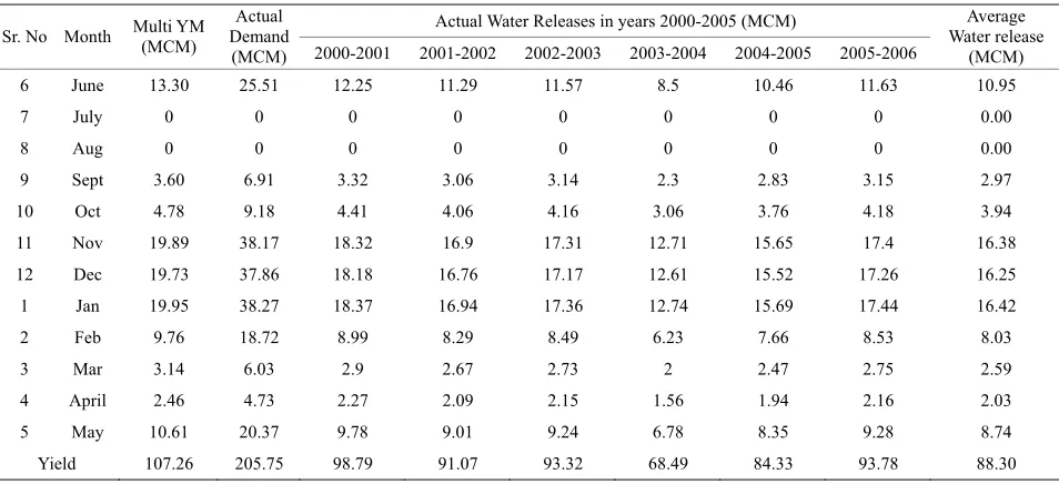
Table 4 gives the output of the model used for 75%
reliable yield as well as demand and actual releases in the years which are considered in Lower Manar-Barul res-ervoir. The data available on actual releases of only 6
years is used for comparison. As per the Table 4 the
ac-tual release from the reservoir is maximum 98.79 MCM in the year 2000-2001 and minimum is 68.49 MCM in
year 2003-2004. Figure 4 shows comparison between
tion by approximate YM (Multi-reservoir) in Manar River.
75% reliable Yield (MCM) θp,j = 0.00 Month Upper Manar
Limboti Reservoir
Lower Manar Barul Reservoir
Total Yield (MCM)
Upper Manar Limboti Reservoir
Lower Manar
Barul Reservoir Total Yield (MCM)
June 1.127 5.302 6.429 2.305 13.301 15.606
July 0.719 0.000 0.719 1.619 0.000 1.619
1.994 0.000 1.994
Sep 3.004 3.206 3.604 6.810
17.352 4.784 22.136
25.170 19.898 45.068
19.239 19.737 38.976
9.030 19.952 28.982
6.799 9.761 16.560
March 3.497 1.253 4.750 7.153 3.143 10.296
A
May 2.8 070 5.801 16.420
Aug 0.975 0.000 0.975
t 1.568 1.436
Oct 8.485 1.907 10.392
Nov 12.308 7.932 20.240
Dec 9.408 7.868 17.276
Jan 4.415 7.954 12.369
Feb 3.324 3.891 7.215
pril 3.702 0.983 4.685 7.571 2.467 10.038
37 4.233 7. 10.619
Total 52.437 42.765 95.207 107.239 107.27 214.515
Table 4. Values of actual demand, actua ses and yield model (YM with 7 able θp,j = 0.0
Actual Water Releases in y s 2000-2005 (MCM
l relea 5% reli 0).
ear )
S Month M )
Actual Demand
(MCM) 2001 2001- 2002-2003 2004 2004- 2006
release M) r. No Multi Y(MCM
2000- 2002 2003- 2005
2005-Average Water
(MC
6 June 13.30 25.51 25 112. 1.29 11.57 8.5 10.46 11.63 10.95
7 July 0 0 0 0 0 0 0 00
Aug 0 0 0 0 0 0 0 00
Sept 6.91 32 3. 3.14 2.3 2. 15 97
Oct 9.18 41 4. 4.16 3.06 3. 18 94
Nov 38.17 32 17.31 12.71 15. 17.4 38
Dec 37.86 18 16. 17.17 12.61 15. 26 25
Jan 38.27 37 16. 17.36 12.74 15. 44 42
Feb 18.72 99 8. 8.49 6.23 7. 53
ar 6.03 9 2.73 2 2. 2.75
4 Apr 2.03
9.78 9. 28
eld 98.79 91. 78
0 0.
8 0 0.
9 3.60 3. 06 83 3. 2.
10 4.78 4. 06 76 4. 3.
11 19.89 18. 16.9 65 16.
12 19.73 18. 76 52 17. 16.
1 19.95 18. 94 69 17. 16.
2 3 M
9.76 3.14
8. 2.
29 2.67
66 8. 47
8.03 2.59
il 2.46 4.73 2.27 2.09 2.15 1.56 1.94 2.16
5 Yi
May 10.61
107.26
20.37 205.75
01 9.24 6.78 8.35 9. 07 93.32 68.49 84.33 93.
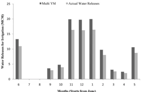
Figure 4. Comparison of ac releases and releases tai fr eld model.
ont ater r , m de and ly
ield by yield model. From the figure it is very clear that in the month of June, December and January the reser-voir releases are comparable with the yield model, where as the actual demand is very large as compared to the actual releases from the reservoir except in the month
February, March and April. It can be seen from the
Fig-ure 4 that the releases are negligible in the period of
Kharif Crop i.e. June, July, August, September and mid
of October. Whereas the releases are more in the period
of Rabbi Crop (i.e. from October to February) and in Hot
Weather crop period (i.e. from February to May).
The Yield model can be used for yield assessment with specified reliabilities and thus assists in the effectiv
istic full optimization model by the way of reduction in
l h o ie o
whic fe r yield model and yield
l with reliab f flow mplete failure.
I he case of complete failure, the annual firm
pro-v ed is zero uring the lure year he yield el is
le of considering reliabi f annua d. It
in the co of com e or partial failure
g the years he yield model for rvoir
m developed in th addresses the
ts of orati esi iabiliti
purp as we all deficit criterion
nnual ation target in a r oir syst
con-g of a M lti reser rrigati stem. It can act as
tter scr g tool ing. Being an op tion
el, no in licy is eeded for the analysis of
res-ir syst e m is gen nough ould
ilar re ir sys
REFERENCES
tual
ob-ned om yi
m hly w eleases onthly mand month
y
e management and design of irrigation reservoir system. Yield model provides a better alternative to the determi-n
size and provides sufficiently accurate results. It also allows determination of annual yield with a given reli-ability less than the maximum relireli-ability. There is also a provision of determining the percentage of annual yield to be supplied during failure years.
4. Conclusion
The study of multi-reservoir operation in Manar River is carried out using LP based yield model. Identification and screening of the feasible solution to provide potential candidates for detailed evaluation is a crucial stage dur-ing the search for optimal solution of real life problems. Mathematical optimization models play a vital role in this regard. The overall effort in handling real life sys-tems can be significantly reduced with screening models capable of better representing the system and providing fewer and more accurate candidate solutions for detailed evaluation which is proportional to the number of candi-date solutions to be evaluated and their proximity to the
optima solution. T e yield m del is stud d for the tw cases,
mode
h are sa 75%
reservoi
ility o with co
n t yield
id d fai s. T mod
capab the lity o l yiel
can also clude ncept plet
durin syste
failure . T
is study successfully
rese
aspec incorp ng the d red rel es for
ferent oses, ll as an owable
for a irrig eserv ems
sistin u voir i on sy
a be eenin in plann timiza
mod ervo
itial po ems. Th
n
odel eral e and c
be applied to sim servo tems.
[1] D. P. Loucks, “Computer Models for Reservoir Regula-tion,” Journal of the Sanitary Engineering Division, Vol. 94, No. 4, 1968, pp. 657-671.
[2] G. C. Dandy, M. C. Connarty and D. P. Loucks, “Com-parison of yield assessment of multiple reservoir sys-tems,” Journal of Water Resources Planning and Man-agement, Vol. 123, No. 6, 1997, pp. 350-358.
[3] W. W. G. Yeh, “Reservoir Management and Operation s Models: A State-of-the-Art Review,” Water Resources Research, Vol. 21, No.12, 1985, pp. 1797-1818.
doi:10.1029/WR021i012p01797
[4] J. W. Labadie, “Optimal Operation of Multireservoir Systems: State-of-the-Art Review,” Journal of Water Resources Planning and Management, Vol. 130, No. 2, 2004, pp. 93-111.
doi:10.1061/(ASCE)0733-9496(2004)130:2(93)
[5] A. K. Sinha, B. V. Rao and U. Lall, “Yield Model for Screening Multi Purpose Reservoir Systems,” Journal of Water Resources Planning and Management, Vol. 125, No. 6, 1999, pp. 325-332.
doi:10.1061/(ASCE)0733-9496(1999)125:6(325)
[6] P. D. Dahe and D. K. Srivastava, “Multipurpose Multi-yield Model with Allowable Deficit in Annual Yield,” Journal of WRPM, Vol. 128, No. 6, 2002, pp. 406-414. [7] D. K. Srivastav and T. A. Awchi, “Storage-Yield
Evalua-tion and OperaEvalua-tion of Mula Reservoir, India,” Journal of Water Resources Planning and Management, Vol. 135, No. 6, 2009, pp. 414-425.
doi:10.1061/(ASCE)0733-9496(2009)135:6(414)
Appendix: Notation
The following symbols are used in this paper: ,
1f p
Oy Annual firm Upper Manar reservoir yield.
, 2
f p
Oy Annual firm Lower Manar reservoir yield.
o 1, 1j
s Initial storage of Upper Manar reservoir at
the beginning of year j.
Initial storage of Lower Manar reservoir at the
g of year j.
begin-r at the
1,j
year j.
2,j
Sp Excess release in Lower Manar reservoir in
year j.
1,j
I Annual inflow at Upper Manar reservoir site in
year j.
2,j
I Annual inflow at Upper Manar reservoir site in
year j.
nin
o 1,j
s Final storage of Upper Manar reservoir at the
beginning of year j.
o 2,j
s Final storage of Lower Manar reservoi
beginning of year j.
Sp Excess release in Upper Manar reservoir in
1,j, 2,j
El El = Annual evaporation volume loss from
reservoir in year j.
1t, 2t
El El = Evaporation volume loss from reservoir in
period t.
1,t, 2,t
= Fraction of total annual yield for assumed
critical period inflow in Uppe Manar reservoir and Lower Manar reservoir.
1, 2
Y Y = Over-year storage capacity of Upper Manar
reservoir and Lower Manar re ,
Ya Ya = Total active storage capacity of
servoir.
Upper
1 2
Manar reservoir and Lower Manar reservoir.
1,t, 2,t
K K = Percentage fraction of annual irrigation
target in period t in Upper Manar and Lower Manar
res-ervoir.
1, 1, 2, 1
w w
t t
s s = Initial within-year storage volume in
pe-riod t in Upper Manar reservoir and Lower Manar reser-voir.
1, w t
s = Final within-year storage volume in period t in
Upper Manar reservoir.