Dynamic Contracting with Persistent Shocks

Munich Personal RePEc Archive

Dynamic Contracting with Persistent

Shocks

Zhang, Yuzhe

University of Iowa

2009

Online at

https://mpra.ub.uni-muenchen.de/23108/

Dynamic Contracting with Persistent Shocks

∗

Yuzhe Zhang

September 30, 2008

Abstract:

In this paper, we develop continuous-time methods for solving dynamic principal-agent problems in which the agent’s privately observed productivity shocks are persistent over time. We characterize the optimal contract as the solution to a system of ordinary differential equations and show that, under this contract, the agent’s utility converges to its lower bound—immiserization occurs. Unlike under risk-neutrality, the wedge between the marginal rate of transformation and a low-productivity agent’s marginal rate of substitution between consumption and leisure will not vanish permanently at her first high-productivity report; also, the wedge increases with the duration of a low-productivity report. We apply the methods to numerically solve the Mirrleesian dynamic taxation model, and find that the wedge is significantly larger than that in the independently and identically distributed (i.i.d.) shock case.

JEL Classification Numbers: D80, D82, E61.

Keywords and Phrases: Persistence, Principal-agent Problem, Stochastic Control Problem, Efficiency Lines.

∗_{I are grateful to the editor, three anonymous referees, Andrew Atkeson, April Franco, Hari Govindan, Roozbeh}

Hos-seini, Marek Kapicka, Ayca Kaya, Patrick Kehoe, Dirk Krueger, Narayana Kocherlakota, Fernando Leiva, Erzo Luttmer,

Ellen McGrattan, Harry Paarsch, Elena Pastorino, Chris Phelan, B. Ravikumar, Larry Samuelson, Yuliy Sannikov, Martin

Schneider, Aleh Tsyvinski, Galina Vereschagina, Noah Williams, Mark Wright, Ivan Werning, Heng-fu Zou, and

espe-cially V.V. Chari and Larry Jones for their helpful comments. I also thank Anita Todd for her excellent proofreading.

All remaining errors are my own.

†_{Department of Economics, Henry B. Tippie College of Business, University of Iowa, Iowa City, IA, 52242, U.S.A.;}

1. Introduction

A common assumption in the dynamic mechanism design literature is that the agent’s privately observed shocks are independently and identically distributed (i.i.d.). As pointed out by Fernandes and Phelan (2000), this assumption is merely for the sake of tractability. It implies that, at the beginning of a given date, an agent’s forward-looking utility of following a given strategy when facing a given contract is independent of past histories.1

However, in many economic environments with hidden information, the agent’s shocks are highly persistent. For example, in the design of optimal health insurance, a customer’s health condition today is strongly correlated with her previous condition. And in unemployment insurance where an unemployed worker’s searching effort is hidden, it is reasonable to conjecture that the worker’s chance of finding a new job depends not only on her current effort but also on her searching effort in the past.

In this paper, we develop continuous-time methods for solving dynamic contracting problems and apply them to an optimal taxation model in which the agent’s privately observed productivity shocks are persistent over time. Productivity process is modeled as a finite-state Markov chain with transitions arriving as a Poisson process. A key technique that we develop is that, in continuous time, the incentive constraints are transformed into a system of differential equations and inequalities. This system of equations connects the principal’s choice variables and the evolution of the promised utilities, thus allows us to rewrite the contracting problem as a stochastic control problem. We then study the stochastic control problem and obtain a sharp characterization of the optimal contract.

We find that the cost of delivering a utility vector is increasing in the promised utility but decreasing in the transitional utility. We also find that for each level of promised utility to the low-productivity agent, there is an efficient (cost-minimizing) level of transitional utility. However, when the agent reports low productivity, the principal has to move the transitional utility strictly below the efficient level, since the high-productivity type has an incentive to misreport and reduce her effort. This feature makes the persistent shock contract open to renegotiation, because moving back to the efficiency level makes the agent indifferent and the principal strictly better off. This is different from the i.i.d. shock case, where the contract is always renegotiation proof.

There are many features that persistent shock models share with i.i.d. shock models. The agent’s promised utility moves up with a high report and moves down with a low report. The consumption and output levels for a high report are both higher than those for a low report when compared at similar levels of promised utilities. The immiserization result continues to hold in persistent shock models, because the martingale property (associated with the inverse Euler equation) remains valid.2

1

This notion of common knowledge about preferences was first discussed in Fudenberg, Holmstrom, and Milgrom

(1990). 2

Based on these findings, we conclude that,qualitatively, the persistent shock models are similar to i.i.d. shocks. However,quantitatively, persistence is still an important issue that should not be ignored. Through a numerical example, we find that the distortions in the persistent shock model are much larger than in the i.i.d. shock model. Thus, using i.i.d. shocks as an approximation to the true productivity shocks would seriously underestimate the role of the tax system in a Mirrleesian model.

1.1

Related Literature

Our formulation of the problem is based largely on ideas in Fernandes and Phelan (2000). They developed a recursive formulation for contracting problems in which private types are serially corre-lated. In these situations, different types of agents derive different continuation utilities from the same continuation contract due to type-specific priors. When the agent chooses between truth-telling and lying, she compares the continuation utility as a truth-teller and the continuation utility as a liar. Thus, the principal finds it necessary to enforce a vector of utilities for all the potentially different types. They showed that this vector of continuation utilities is the state variable in their recursive formulation. Our work provides an analytical characterization of the optimal contract, which is different from Fernandes and Phelan (2000), who solved the optimal contract by numerical iteration following Abreu, Pearce, and Staccheti (1990).

This paper is motivated by the literature on continuous-time contracting with hidden actions (Holm-strom and Milgrom (1987), Schattler and Sung (1993), Cvitanic, Wan, and Zhang (2007), Williams (2006), Westerfield (2006), Sannikov (2007a,b)). The literature shows that setting principal-agent mod-els in continuous time could allow for more explicit characterization of the solution. The novelty in this paper involves our modeling of the random process. Since the traditional continuous-time methods with diffusion process cannot be readily adopted to study hidden information models with persistent shocks (see Section 7 for an explanation), we model the agent’s type as a finite-state Markov chain, which introduces techniques that are different from, but complementary to, the above literature.

inverse Euler equation does not hold in his environment and the immiserization property disappears.3

Finally, our paper is closely related to the literature on dynamic social insurance and taxation (Albanesi (2006), Albanesi and Sleet (2006), Atkeson and Lucas (1992), Golosov, Kocherlakota, and Tsyvinski (2003), Golosov and Tsyvinski (2006, 2007), Kocherlakota (2005), Kapicka (2006)). Our model is a simplified version (with neither aggregate resource constraint nor capital accumulation) of Golosov, Kocherlakota, and Tsyvinski (2003) and Kocherlakota (2005). However, our research focuses more on developing a methodology and understanding the analytical properties of the optimal contract. Battaglini and Coate (2003) studied a persistent shock dynamic taxation model with risk-neutral agents. The distortion in their model eventually vanishes in two senses. First, it vanishes permanently with any high-productivity report. Second, the distortion decreases to zero for an agent who always reports low productivity. We can apply the continuous-time methods to study their model and confirm their findings. However, when we study risk-averse utilities, we find that the distortion increases with the low-productivity report and never vanishes. These differences suggest that risk aversion is critical for the patterns of the distortion.

The remainder of the paper is organized as follows. Section 2 lays out the economic environment and sets up the social planner’s contracting problem. In Section 3, we derive the continuous-time evolution of the state variable as differential equations and inequalities. The resulting differential equations are put to use in Section 4 to characterize the set of implementable utility pairs and in Section 5 to study the long-run dynamics of the optimal contract. In Section 6, through a numerical example, we show that the models with persistent shocks imply significantly larger wedges than the models with i.i.d. shocks. The last section concludes. All proofs are collected in the Appendices.

2. A Dynamic Contracting Problem

2.1

The Environment and the Shock Process

Time is continuous. Consider a risk-neutral principal and a risk-averse agent who engage in long-term contracting at time 0. Both the principal and the agent are able to commit. The preferences of the agent are

E

·Z ∞

0

e−rt[u(ct)−v(yt)/θt]dt

¸

,

(1)

where ct and yt are the agent’s consumption and output at time t, r is her discount rate, θt is her

private taste shock, andEis an expectations operator. The principal has the same discount raterand

3

The first-order approach is able to reduce the dimension of the state variable to a small number, but its validity is

still unestablished. Williams (2008) provided sufficient conditions for the first-order approach, but these conditions may

minimizes

E

·Z ∞

0

e−rt[ct−yt]dt

¸

,

(2)

which is the expected discounted cost of the consumption-output plan. We assume thatu: [0,¯c]→[0,u¯] is twice continuously differentiable, increasing, and strictly concave (u′_{>0 andu}′′_{<0). The disutility}

functionv: [0,y¯]→[0,¯v] is twice continuously differentiable, increasing, and strictly convex (v′_{>0 and}

v′′>0). The agent’s privately observed taste shockθt can be re-interpreted as a productivity shock if

v(y) =yγ_{, γ >1. Defineφ=θ}1/γ _{as the agent’s productivity. She is able to transform one unit of labor}

intoφunits of output. Her disutility depends on the amount of laborl=y/φshe spends to producey, thus the disutility isv(l) =v(y)/θ.

The shock process (θt)t≥0is a time-homogeneous, continuous-time Markov chain with a finite state

space Θ = {θ1, θ2, ..., θN}, where 0 < θ1 < θ2 < ... < θN, and a generator matrixQ = (qij)1≤i,j≤N.

LetN _{={1,2, ..., N} be the set of indices. A probability space (Ω,}F_{, P) is described as follows. Let}

sample space Ω be

n

ω: [0,∞)→N¯¯

¯ ω is right continuous, has a finite number of jumps in any interval [0, t], t≥0 o

.

Each ω ∈ Ω describes a complete sample path of random indices. For t ≥ 0, the random variable

ιt(ω) = ω(t) describes the state at t. To keep track of information, endow Ω with a filtration, i.e., a

nondecreasing family{F_{t}t≥0 ofσ-fields, where} F_{t=σ((ιs)0≤s≤t) and} F _=σ(∪t≥0F_t). F_{t denotes}

the information from 0 up tot, including the number of jumps up tot, the timing, and the destinations of these jumps. The generator matrixQsatisfies the following conditions:

(i) −qii>0 for alli; (For convenience, we useqi to denote −qii)

(ii) qij >0 for all i6=j;

(iii) P

jqij= 0 for alli.

Each entryqij (i6=j) is the rate of moving from stateito statej, andqi=Pj6=iqij>0 is the rate of

leaving statei. For all t, h≥0, conditional onιt=i,

Pr(ιt+h=j|ιt=i) = δij+qijh+o(h),

where δij is 1 if i =j, and 0 otherwise. An equivalent way to describe the continuous-time Markov

chain is that, conditional onιt=i, the holding timeS (which records the duration that the chain stays

inibefore a transition) is an exponential random variable of parameterqi, and once a transition occurs,

it jumps to statej (j6=i) with probabilityqij/qi. We can always endow the measurable space (Ω,F)

with a probability measureP such that underP, (ιt)t≥0 is a Markov chain with the generator matrix

2.2

The Contracting Problem

The agent knows her initial type and privately observes (ιt)t≥0afterwards, while the principal cannot

observe the realizations and holds a belief that the agent’s initial type isiwith probabilitypi, 1≤i≤N.

At time 0, the principal offers a contract, which the agent may either accept or reject. If the agent rejects, then she gets the outside option ¯Uiif her initial type isi. Otherwise, she sequentially reports the

newly observed shocks to the principal, and the principal implements the contract based on reported histories.

In each period t, based on realized shocks (ιs)0≤s≤t, the agent makes a report σt to the principal.

Collectively, with sample pathω realized, the agent’s reported history is σ = (σt)t≥0. Therefore, we

define the agent’s reporting strategy to be a measurable function σ : (Ω,F_{) → (Ω,}F_{). Moreover,}

at time t, since an agent is unable to distinguish between two sample paths ω1_{, ω}2_{, where ω}1_{(s) =}

ω2_{(s),∀s∈[0, t], the reported paths have to satisfy σ(ω}1_{)(s) =σ(ω}2_{)(s),∀s ∈[0, t]. This means that}

σshould also be measurable from (Ω,F_{t) to (Ω,}F_{t) for any t≥0. We could write σt(ω) =σt(ω}[0,t]_),

whereω[0,t] _{is the restriction ofω on [0, t]. Notice that this definition of a reporting strategy implicitly}

imposes restrictions on the agent’s reports; when the reports at different t are pieced together, the reported historyσ(ω) has to be right continuous and admits finite jumps in finite time. This restriction is innocuous. Since the true sample paths have these properties, if the agent cheats and, for example, her reports fail to be right continuous, then cheating will be identified by the principal. Intuitively, right continuity prohibits the agent from immediately reverting to truth-telling after misreporting att, and the finite-jump condition prohibits her from switching between truth-telling and cheating too often. A reporting strategyσ istruth-telling if σ(ω) = ω, for allω ∈Ω. We use σ∗ _{to denote the truth-telling}

strategy.

The principal offers a contract C _{= (ct, yt)t≥0 at time 0, where the measurable functions ct :}

(Ω,F_{t)→[0,c¯] andyt: (Ω,}F_{t)→[0,y¯] specify the agent’s consumption and output at t, respectively.}

We use Ω to denote both the set of true realizations and the set of reports. As a collection of subsets that contain reports, the algebraF_{tdescribes the principal’s information structure; while as a collection of}

subsets that contain the true shocks, it describes the agent’s information structure. When the reporting strategy isσ, the principal’s information in the space of true shocks,σ−1(F_{t) ={A⊆Ω :σ(A)∈}F_t},

is weakly coarser than that of the agent. Here for the principal, Ω is the set of reports and the measurability condition requires that ct andyt be based only upon the reports available from 0 up to

(and including)t. We assume that a contract is progressively measurable; in other words, the mapping (s, ω) →(cs(ω), ys(ω)) : ([0, t]×Ω,B([0, t])⊗Ft)→ (R2,B(R2)) is measurable for all t ≥0.4 Note

that the information structure here is similar to that in the discrete-time literature. Within a period

4

(or instant), the timing is that an agent first makes her report then receives her compensation. In both cases, consumption and output under the contract are allowed to jump instantaneously with the arrival of a new report, rather than being required to be predictable functions of past reports.

It is useful to study the agent’s promised utility vector based on different histories, which turns out to be the state variable in a recursive formulation. Denote the set of possible histories before the realization ofιt by

N t− ₌n_ιt−_{: [0, t)→}N ¯¯ ¯ ι

t− _{is right continuous, has a finite number of jumps}o_.

An agent’s future discounted utility when she has a history of reportsht−_∈N t−_{, her realization ofι}

t

isiand she follows a strategyσis

wi(ht−;σ,C)

= Et

·Z ∞

t

e−r(s−t)hu(cs(ht−,(σ(ω))[t,∞)))−v(ys(ht−,(σ(ω))[t,∞)))/θω(s)

i

ds¯¯

¯ω(t) =i ¸

,

where (σ(ω))[t,∞)_{is the restriction of the reportσ(ω) on [t,∞), and (h}t−_,(σ(ω))[t,∞)_{) denotes a sample}

path (or report) whereht− _{is followed by (σ(ω))}[t,∞)_{. In particular, ifσ=σ}∗_,

wi(ht−;σ∗,C)

(3)

= Et

·Z ∞

t

e−r(s−t)hu(cs(ht−, ω[t,∞)))−v(ys(ht−, ω[t,∞)))/θω(s)

i

ds¯¯

¯ω(t) =i ¸

= Et

·Z ∞

t

e−r(s−t)hu(cs(ht−, ω[t,s]))−v(ys(ht−, ω[t,s]))/θω(s)

i

ds¯¯

¯ω(t) =i ¸

.

It will be crucial to distinguish betweenpersistent promised utility andtransitional promised utilities. The report at an instanttmay either be the same as previous reports or indicate a transition. Accord-ingly, there are two types of promised utilities: the utility associated with no transition and the utilities associated with all possible transitions. More precisely, let i∗

t = lims↑tht−(s) be the report of type

immediately beforet. Thenwi∗

t(h

t−_;σ∗_{,C) is called thepersistent promised utility andw}

i(ht−;σ∗,C),

(i6=i∗

t), are called thetransitional promised utilities. When the agent’s current report is the same as

the previous reports, she receives the persistent promised utility; otherwise, if there is a transition to statei, she receiveswi(ht−;σ∗,C). Detailed discussion of the promised utilities is provided in the next

section.

A contractC _{is said to beincentive compatible(I.C.) if for anyt, anyh}t−_∈N t−_{, and any strategy}

σ,

wi(ht−;σ∗,C) ≥ wi(ht−;σ,C), for alli.

(4)

attention to I.C. contracts. The principal’s problem can then be written as minC

N

X

i=1

piE

·Z ∞

0

e−rt[ct(ω)−yt(ω)]dt

¯ ¯

¯ω(0) =i ¸

(5)

subject to C _{is I.C.,}

wi(∅;σ∗,C)≥U¯i, for alli,

where∅ denotes an empty history and ¯Ui is the typeiagent’s outside option.

3. Incentive Constraints and the Evolution of

(

w

₍

h

₎₎

1≤i≤N

In this section, we show that (wi(ht−;σ∗,C))1≤i≤N is the state variable for a dynamic programming

problem, and that the incentive constraints can be simplified as differential equations (and inequalities) that describe the evolution of the state variable.

In the following discussion, the discounted utilitywi(ht−;σ∗,C) will be simplified towi(ht−) when

σ∗ _{and C are well understood. i}[t,s) _{denotes a sample path (or report) of type i from t to s (not}

includings).

Fix an I.C. contractC_{. First, consider the continuity property ofwi(h}t−_{) as a function oft. Recall}

thati∗

t denotes the report immediately beforet. When limits are taken from the left,wi∗

t is the persistent promised utility and other wi (i6=i∗t) are transitional promised utilities. Things become complicated

when limits are taken from the right, since there are N possible paths of reports. Starting from t, the agent might report i = i∗

t, which the principal interprets as no transition, or she might report

i6=i∗

t, which the principal interprets as a transition toi. Following history (ht−,(i∗t)[t,s)),wi∗

t is still the persistent promised utility. However, following (ht−_{, i}[t,s)_{) (i6=i}∗

t),wi would replacewi∗

t to be the persistent promised utility.

The following lemma shows that the persistent promised utility is continuous, while the transitional promised utilities have both left and right limits but allow for downward jumps.

Lemma 1 If C _{is I.C., then}

(i) For right-hand limits,

wi(ht−) = lim s↓twi(h

t−_{, i}[t,s)_{), for alli,} (6)

wj(ht−) ≥ lim s↓twj(h

t−_{, i}[t,s)_{), for allj 6=i.} (7)

(ii) For left-hand limits, let hs− _{denote the restriction of h}t− _{on [0, s) (s < t),}

wi∗

t(h

t−_{) = lim}

s↑twi

∗

t(h

s−_), (8)

wj(ht−) ≤ lim s↑twj(h

s−_{), for allj6=i}∗

t.

It is useful to understand the meaning of equation (7) with various values of i and j. If j 6=i∗

t (she

has a transition toj), then she could not gain by delaying the transition report and reportingi∗

t for a

short time (followed by truth-telling), or by reporting a transition to a different statei (i6=j, i6=i∗

t)

for a short time (followed by truth-telling). Ifj =i∗

t (she does not have a transition), then she could

not gain by reporting a transition to i(i6=i∗

t) for a short time (followed by truth-telling).5 Similarly,

equation (9) simply means that an agent with a transition tojbeforet would not delay the transition report untilt.

Next we will obtain a sharper characterization of the evolution of utility wi along any reported

history. Fix a reportht−_{. It follows from the definition ofN} t− _{that there exists a finite collection of}

jump timest0= 0< t1< t2< ... < tn < tn+1=t and a finite history of past types (i0, i1, ..., in), such

that ht−_{(s) =i}

k, ifs∈[tk, tk+1), 0≤k≤n. In the interval [tk, tk+1),wik is the persistent promised utility and, in addition to being continuous, its evolution is described by a differential equation. wi

(i6=ik) is a transitional promised utility in [tk, tk+1). Although it could have a countable number of

downward jumps, its evolution is described by a differential inequality (an upper bound on dwi/dt is

found). These differential equations (and inequalities) are both necessary and sufficient conditions for a contract to be I.C. We turn next to this key characterization result.

Theorem 1 Let C _{be a contract, and (wi(h}t−₎₎

1≤i≤N, (wi(ht−) : N t− → R, for all t ≥ 0), be an arbitrary stochastic process.

(i) (necessity) If C _{is I.C., and (wi(h}t−₎₎

1≤i≤N are the promised utilities defined in (3), then for

any history ht− with the form (t0, t1, ..., tn, tn+1;i0, i1, ..., in), wi(hs−) is differentiable for all i and almost every (a.e.) s∈[0, t). Ifi=ik, then for a.e. s∈[tk, tk+1),

dwi(hs−)

ds = (r+qi)wi(h

s−₎₋X

j6=i

qijwj(hs−)−(u(c(hs))−v(y(hs))/θi).

(10)

If i6=ik, then for a.e. s∈[tk, tk+1),

dwi(hs−)

ds ≤ (r+qi)wi(h

s−₎₋X

j6=i

qijwj(hs−)−(u(c(hs))−v(y(hs))/θi).

(11)

(ii) (sufficiency) Assume (wi(ht−))1≤i≤N is a bounded process and for any history ht− with the form (t0, t1, ..., tn, tn+1;i0, i1, ..., in), wi(hs−) is differentiable for all i and a.e. s ∈ [0, t). If

(wi(ht−))1≤i≤N and C satisfy (10) and (11), then (wi(ht−))1≤i≤N satisfies (3), and contractC is I.C.

5

It is helpful to understand the meanings of (10) and (11), because all of our remaining results are derived from this system of differential equations and inequalities. Equation (10) is apromise-keeping

condition. We can rewrite the right side of equation (10) as

£

rwi(hs−)−(u(c(hs))−v(y(hs))/θi)

¤

+

 

X

j6=i

qij(wj(hs−)−wj(hs−))

 ,

where the first term is the natural (instantaneous) rate of change of promised utility wi(hs−) when

there is no uncertainty. For j 6=i, each term qij(wi(hs−)−wj(hs−)) captures the additional rate of

change ofwi(hs−) due to the transition to statejat arrival rateqij. The promise-keeping condition in

discrete time is

wi(s) = (u(c(s))−v(y(s))/θi)dt+e−rdt



 X

j6=i

(qijdt)wj(s+dt) +e−qidtwi(s+dt)



,

(12)

wheresands+dtdenote two periods in discrete time andqijdtis the transitional probability in short

timedt. Equation (10) can be informally derived by taking limitdt→0 in (12). (The formal proof can be found in APPENDIX A.) Inequality (11) is anincentive compatibility condition, the intuition for which is similar to that of (10). If (11) holds as equality, then typei obtainswi(hs−) by reportingik,

thus she is indifferent between truth-telling and reportingik; otherwise, ifwi(hs−)/ds is less than the

right side of (11), then reportingik makes her strictly worse off.

With the conditions on the derivatives of (wi(ht−))1≤i≤N, the principal’s problem is transformed

into a dynamic stochastic control problem. With truth-telling, (wi(ιt−))1≤i≤N andιtare endogenous

and exogenous state variables, respectively, and (ct, yt) are control variables. Given the current reporti

and before the next transition, the system evolves according to a differential inclusion (in the following discussion,wi(ht−),c(ht), andy(ht) will be simplified towi(t) (orwi),ct, andytwhenht− andht are

well understood):

dwi

dt = (qi+r)wi−

X

j6=i

qijwj−u(ct) +v(yt)/θi,

dwj

dt ∈



−∞,(qj+r)wj−

X

k6=j

qjkwk−u(ct) +v(yt)/θj



, j6=i.

Introducing (N−1) slack control variablesµj,µj ≥0,j6=i, the system is

dwi

dt = (qi+r)wi−

X

j6=i

qijwj−u(ct) +v(yt)/θi,

dwj

dt = (qj+r)wj−

X

k6=j

qjkwk−u(ct) +v(yt)/θj−µj, j6=i.

When a downward jump ofwjhappens, we interpret it asµj =∞. Given initial statesiand (wj)1≤j≤N,

the costVi((wj)1≤j≤N) is

Vi((wj)1≤j≤N) =E

·Z ∞

0

e−rth_c

t(ω[0,t])−yt(ω[0,t])

i

dt¯¯

¯ω(0) =i ¸

.

(Vi)1≤i≤N can be directly used to solve the principal’s problem in (5). If the prior belief is degenerate,

(pi= 1, pj= 0,∀j 6=i, i.e., initial type is known to the principal), then the principal can pick an initial

state (wj)1≤j≤N to start the optimal control problem; except the participation constraint wi ≥ U¯i,

the other states wj(j 6=i) are transitional utilities, and are free to be chosen by the principal. When

the prior belief is not degenerate, the principal can choose a type-dependent state variable to start the optimal control problem: when the initial report isi, the principal picks an initial state (wi

j)1≤j≤N. To

prevent a typeiagent from misreportingj and immediately reporting a transition toi, and obtaining the transitional promised utilitywji, the incentive constraintswii≥w

j

i must be imposed. To summarize

the above discussion, the principal’s problem in (5) is equivalent to

min

(wi j)1≤i,j≤N

N

X

i=1

piVi((wji)1≤j≤N)

subject to wii≥U¯i,

wii≥w j

i, for alli, j.

Remark 1 The conditions in (10) and (11) are still necessary when the instantaneous utility function is unbounded. However, for sufficiency, some form of transversality condition is needed. One sufficient condition is that, for any reporting strategyσ,

lim

t→∞e

−rt_Eh_w

ιt((σ(ω))

[0,t)₎i _{= 0.}

4. The Set of Implementable Utilities

To simplify the exposition, in the remainder of the paper we will consider only the case in which

N = 2. This section studies the set of implementable utilities, defined as,

W =©

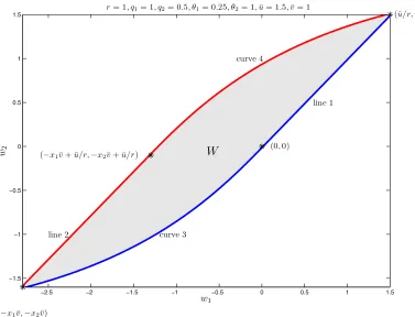
(w1(∅;σ∗,C), w2(∅;σ∗,C))∈R2:C is I.C.ª,

which is the domain of the value functions. In the next section, we examine the properties of the value functions and the long-run dynamics implied by them.6

6

Both of these sections use the differential equations we developed earlier heavily; however, there is not much

depen-dence between them, and either one could be read first. In the next section, we focus mainly on unbounded utility and

disutility functions, andW with unbounded utilities is much easier to obtain than with bounded utilities (in the next section,W is the whole setR2

The common approach in the literature is to compute this set by iteration. Following Abreu, Pearce, and Staccheti (1990), begin with an initial guess that containsW, then iterate until the sequence of sets converges toW, which is the largest fixed point of the operator. However, using continuous-time meth-ods, we will show that this set can be obtained directly. In fact the boundary ofW can be characterized by differential equations. The remainder of this section will be devoted to this characterization.

We first study some simple contracts. If the contract always specifies maximal consumption ¯c and minimal output 0, regardless of reports (i.e.,ct(ht) = ¯c, yt(ht) = 0,∀ht ∈Nt), then the contract can

implement the pair (¯u/r,u/r¯ ), which is the upper-right corner ofW. If consumption 0 and output ¯y

are always specified, then the lower-left corner is implemented. We denote it by −(x1v, x¯ 2v¯), where

x1= ((q2+r)/θ1+q1/θ2)/(r(q1+q2+r)), x2= (q2/θ1+ (q1+r)/θ2)/(r(q1+q2+r)). Similarly, the

“consumption 0, output 0” contract implements the utility pair (0,0), while the “consumption ¯c, output ¯

y” contract implements (−x1v¯+ ¯u/r,−x2¯v+ ¯u/r).

Next consider four families of contracts. The first two families are indexed byc∗_{∈(0,¯c). A contract}

C1c∗ _{in the first family is (c}1_tc∗_(ht_{), yt}1c∗_(ht_{)) = (c}∗_{,0), for allh}t_∈ N t_{, which implements the utility}

pair

(u(c∗)/r, u(c∗)/r), c∗∈(0,¯c).

(13)

A contractC2c∗

in the second family is (c2c∗

t (ht), y2c

∗

t (ht)) = (c∗,y¯), for allht∈N t, which implements

the utility pair

(−x1v¯+u(c∗)/r,−x2v¯+u(c∗)/r), c∗∈(0,¯c). (14)

The third and fourth families of contracts are indexed by t∗ _{∈ (0,∞). A contract C}3t∗

in the third family is

(c3tt∗(ht), y3t

∗

t (ht)) =

  

 

(0,0), t≤t∗

(0,y¯), t > t∗_,

while in the fourth family, a contractC4t∗

is

(c4tt∗(ht), y4t

∗

t (ht)) =

  

 

(¯c,y¯), t≤t∗

(¯c,0), t > t∗_.

The utility pair (w3t∗

1 , w3t

∗

2 ) implemented byC3t

∗

can be solved in the following way. Under contract

C3t∗

, and whent≤t∗_{, the promised utility evolves according to the differential equation system}

dw1

dt = (q1+r)w1−q1w2 dw2

and (w1, w2) will hit (−x1v,¯ −x2¯v) at time t∗. Therefore, solving the differential equations together

with the boundary condition yields

w13t∗ =−¯v

·

q1(1/θ1−1/θ2)

(q1+q2)(q1+q2+r)

e−(q1+q2+r)t∗₊q2/θ1+q1/θ2

(q1+q2)r

e−rt∗

¸

,

(15)

w23t∗ =−¯v

· _q

2(1/θ2−1/θ1)

(q1+q2)(q1+q2+r)e

−(q1+q2+r)t∗₊q2/θ1+q1/θ2

(q1+q2)r e −rt∗¸

.

(16)

Similarly,

w14t∗ = ¯v

·

q1(1/θ1−1/θ2)

(q1+q2)(q1+q2+r)

e−(q1+q2+r)t∗₊q2/θ1+q1/θ2

(q1+q2)r

e−rt∗

¸

−x1¯v+ ¯u/r, (17)

w24t∗ = ¯v

·

q2(1/θ2−1/θ1)

(q1+q2)(q1+q2+r)

e−(q1+q2+r)t∗₊q2/θ1+q1/θ2

(q1+q2)r

e−rt∗

¸

−x2¯v+ ¯u/r. (18)

It turns out that the utility pairs delivered by (C1c∗_,C2c∗_,C3t∗_,C4t∗_{) form the boundary ofW (see}

Figure 1).

−2.5 −2 −1.5 −1 −0.5 0 0.5 1 1.5

−1.5 −1 −0.5 0 0.5 1 1.5

w1

w2

r= 1, q1= 1, q2= 0.5, θ1= 0.25, θ2= 1,u¯= 1.5,v¯= 1

W

(−x1¯v,−x2v¯)

line 1

line 2

(0,0)

curve 3

curve 4

(−x1¯v+ ¯u/r,−x2¯v+ ¯u/r)

(¯u/r,¯u/r)

Figure 1: The set of implementable utility pairs.

Theorem 2 The boundaries of W consist of the four points (¯u/r,u/r¯ ), (−x1¯v,−x2v¯), (0,0), and

(−x1¯v+ ¯u/r,−x2¯v+ ¯u/r), and the four pieces of curves that connect these points. The lower boundary

is specified in equations (13), (15), and (16), while the upper boundary is specified in equations (14),

It is intuitive that curves in (14), (17), and (18) specify the upper boundary. Since for a fixedw1, in

order to increase w2, the principal could increase consumption and output in a way that makes the

low-productivity agent indifferent but the high-productivity agent better off, it is not surprising to see that, at curves on the upper boundary, output is maintained at the maximum level ¯y. Similarly, output is at the minimum level 0 on the lower boundary.

Remark 2 When utility is unbounded, it is typically easier to determineW. For example, when utility and disutility can take any real number, consider the no-information contract, where constant c∗ _and

y∗ _{are specified regardless of reports. This is trivially I.C. and delivers utility}





w1

w2



= 



1/r −x1

1/r −x2



 



u(c∗₎

v(y∗₎



,

where x1=

(q2+r)/θ1+q1/θ2

r(q1+q2+r)

, x2=

q2/θ1+ (q1+r)/θ2

r(q1+q2+r)

.

Since the matrix has full rank, any (w1, w2) ∈ R2 can be implemented by choosing the appropriate

u(c∗_{) andv(y}∗_{). Therefore,W =R}2 _{in this case.}

5. Dynamics of the Optimal Contract

In previous sections, we simplified the incentive constraints and used them to characterize the set of implementable utility pairs. In this section, we address the question of the dynamic behavior of the state variables under the optimal contract. To simplify the analysis, we focus on a special case where the shock space consists of two elements, Θ ={θ1, θ2}, θ1 < θ2, and the agent has logarithmic utility

and disutility functions,u(c) = log(c), c >0, andv(y) =−log(−y), y <0. We assume that the value functions V1 and V2 in this case aretwice differentiable and an optimal contract always exists for any

utility pair (w1, w2). We use Vi,1, Vi,2, Vi,11, Vi,12, Vi,22 to denote ∂w∂Vi1,

∂Vi

∂w2,

∂2_V

i

∂w1∂w1,

∂2_V

i

∂w1∂w2,

∂2_V

i

∂w2∂w2,

respectively, fori= 1,2.

It is helpful to first preview this lengthy section. We find two parallel efficiency lines, which separate the state space R2 into three regions. We then show that the bottom region is absorbing. With a high-productivity report, the state variable moves upward and along the efficiency line, while with a low-productivity report, the state variable moves downward and enters the interior of the region. The dynamics of the system are described by an ordinary differential equation (ODE) system, and by studying the system, we derive many sample path properties, which are summarized inTheorem3.

Consider first the homogeneity of the value functions. It follows from log(exp(λ)c) =λ+ log(c) that a contractC _{= (ct, yt)t≥0 implements (w1, w2), if and only if (exp(λ)ct,exp(λ)yt)t≥0 implements}

wherex1= ((q2+r)/θ1+q1/θ2)/(r(q1+q2+r)), x2= (q2/θ1+ (q1+r)/θ2)/(r(q1+q2+r)). Therefore,

(c∗

t, yt∗)t≥0 is the optimal contract to implement (w1, w2) if and only if (exp(λ)c∗t,exp(λ)y∗t)t≥0 is the

optimal contract at (w1+ (1/r+x1)λ, w2+ (1/r+x2)λ). Moreover, the speed vectors of the time paths

starting from these two initial conditions are identical, i.e., for (w′

1, w2′) = (w1+ (1/r+x1)λ, w2+ (1/r+x2)λ),

dw1(i[0,t))

dt =

dw′ 1(i[0,t))

dt ,

dw2(i[0,t))

dt =

dw′ 2(i[0,t))

dt , i= 1,2.

(19)

The next lemma states this homogeneity and uses it to establish other elementary properties ofV1

andV2.

Lemma 2 The value functionsV1, V2 have the following properties:

(i) (Homogeneity) For any λ∈R,

Vi(w1+ (1/r+x1)λ, w2+ (1/r+x2)λ) = exp(λ)Vi(w1, w2), i= 1,2; (20)

(ii) V1 andV2 are weakly convex;

(iii) (Monotonicity)V1,2≤0, V1,1>0, V2,1≤0, V2,2>0.

Part (iii) of the above lemma states that value functions are monotonic, increasing in the persistent promised utility but decreasing in the transitional utility. The transitional utility is used as a threat: it is what a cheater can hope to get if she pretends to be the reported type but immediately reports a transition to her true type afterwards. For this reason, the transitional utility is also called thethreat

utility. The monotonicity in the persistent promised utility is straightforward because the principal needs to give more consumption to (and require less output from) the agent if he promises more expected utility to her. The intuition forV1,2≤0 is as follows. The principal can instantaneously and

freely lower the transitional utility and keep a tighter threat at zero cost; however, once the transitional utility is moved to a lower level, it is not I.C. to jump back immediately. Thus the cost function cannot be increasing in the transitional utility. Next we will show that it is strictly decreasing when the transitional utility is sufficiently low, i.e., for aw1,V1,2<0 ifw2 is sufficiently low.

Lemma 3 For all w1∈R,{w2 ∈R:V1,2(w1, w2)<0} 6=∅, {w2∈R:V1,2(w1, w2) = 0} 6=∅. And for

allw2∈R,{w1∈R:V2,1(w1, w2) = 0} 6=∅,{w1∈R:V2,1(w1, w2)<0} 6=∅.

SinceV1,2≤0,V1, as a function ofw2, could be strictly decreasing forever or be flat forever. The above

lemma rules out these two possibilities and, together with the convexity ofV1, it implies that there is

an intermediate level ofw2, below which the value functionV1is strictly decreasing and above which it

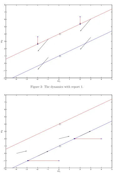
is flat. Formally, we can define two curves,f1 andf2:

f1(w1) = min{w2∈R:V1,2(w1, w2) = 0},

Since V1,2(w1, w2) = 0 if and only if V1,2(w1+ (1/r+x1)λ, w2+ (1/r+x2)λ) = 0, it follows that f1

and f2 are parallel straight lines with slope (1/r+x2)/(1/r+x1). We call f1 and f2 the efficiency

lines, because for each level of promised utility, they indicate the optimal level of transitional utility to minimize the cost. For example, if initially the principal holds the beliefp1= 1 and he wants to deliver

utilityw1to the agent, then he needs to choose a transitional promised utility as one of the initial state

variables. The optimal level to choose isw2=f1(w1).

These lines are also critical for the study of the dynamics. Starting from abovef1, the state variable

will jump downward to the efficiency line f1 with a report 1, and starting from below f2, the state

variable will jump leftward to f2 with a report 2. We further show that, although the transitional

utility might make downward jumps contingent on the report of a transition, it never jumps when the report remains unchanged. When it jumps with a report of transition, it always jumps onto the efficiency lines and stays below them until another transition occurs. The fact that the time path is smooth when there is no transition is intuitive; since the utility function is strictly concave, making abrupt changes in transitional utilities without arrival of new information increases the cost for the principal. The properties of the time path of the state variable are summarized in the following lemma.

Lemma 4 For a reported historyht−_{, ifw}

2(ht−)> f1(w1(ht−)),

lim

s↓tw2(h

t−_,1[t,s)_{) = f}

1(w1(ht−)).

Furthermore,w2(ht−,1[t,s))is a continuous function ofs∈(t,∞), so that bothw1andw2are continuous

following the path of(ht−_,1[t,s)_{). Similarly, ifw}

1(ht−)> f2(w2(ht−)),

lim

s↓tw1(h

t−_,2[t,s)_{) = f}

2(w2(ht−)).

The definition of efficiency lines and the immediate jumps make it clear that

V1(w1, w2) = V1(w1,min(w2, f1(w1))),

V2(w1, w2) = V2(min(w1, f2(w2)), w2).

In the region below the efficiency lines, no further jumps occur in the state variable. Since the evolution of the state variable is controlled by differential equations in this region, one can lay out theHamilton– Jacobi–Bellman (HJB)equations that the value functions satisfy.7 _{For any (w}

1, w2) withw2≤f1(w1),

V1satisfies

(q1+r)V1(w1, w2) = min

c {c−(V1,1+V1,2)u(c)}+ miny {−y+ (V1,1/θ1+V1,2/θ2)v(y)}

+q1V2(w1, w2) +V1,1((q1+r)w1−q1w2)

+ min

µ2≥0

{V1,2((q2+r)w2−q2w1−µ2)}. (21)

7

See, for example, Fleming and Soner (2006, equation (7.13), p.134), or see W¨alde (2006) for a general reading on

Similarly, for (w1, w2) withw1≤f2(w2),

(q2+r)V2(w1, w2) = min

c {c−(V2,1+V2,2)u(c)}+ miny {−y+ (V2,1/θ1+V2,2/θ2)v(y)}

+q2V1(w1, w2) + min

µ1≥0

{V2,1((q1+r)w1−q1w2−µ1)}

+V2,2((q2+r)w2−q2w1).

In addition, notice thatµ2 (µ1) can be non-zero only ifV1,2= 0 (V2,1= 0). Therefore, ifw2< f1(w1),

we can rewrite the HJB equation as (q1+r)V1(w1, w2) = min

c {c−(V1,1+V1,2)u(c)}+ miny {−y+ (V1,1/θ1+V1,2/θ2)v(y)}

+q1V2(w1, w2) +V1,1((q1+r)w1−q1w2)

+V1,2((q2+r)w2−q2w1).

Totally differentiating (21) with respect tow1and applying the envelop theorem yield

(q1+r)V1,1 = −(V1,11+V1,12)u(c) + (V1,11/θ1+V1,12/θ2)v(y)

+q1V2,1+V1,1(q1+r) +V1,11((q1+r)w1−q1w2)

−V1,2q2+ min

µ2≥0

{V1,12((q2+r)w2−q2w1−µ2),

which is simplified as

0 = V1,11((q1+r)w1−q1w2−u(c) +v(y)/θ1)

+V1,12((q2+r)w2−q2w1−u(c) +v(y)/θ2−µ2) +q1V2,1−q2V1,2.

Usingdw1/dt= ((q1+r)w1−q1w2−u(c)+v(y)/θ1), anddw2/dt= ((q2+r)w2−q2w1−u(c)+v(y)/θ2−µ2),

we get

dV1,1

dt = V1,11 dw1

dt +V1,12 dw2

dt =q2V1,2−q1V2,1.

Similarly, totally differentiating (21) with respect tow2 yields

dV1,2

dt = q1V1,1−q1V2,2+ (q1−q2)V1,2.

The above equations together with dw1/dt = ((q1+r)w1−q1w2−u(c) +v(y)/θ1), dw2/dt= ((q2+

r)w2−q2w1−u(c) +v(y)/θ2−µ2) constitute an ODE system to describe the dynamics with report 1:

dw1

dt = (q1+r)w1−q1w2−u(c) +v(y)/θ1

(22)

dw2

dt = (q2+r)w2−q2w1−u(c) +v(y)/θ2−µ2

(23)

dV1,1

dt = q2V1,2−q1V2,1

(24)

dV1,2

dt = q1V1,1−q1V2,2+ (q1−q2)V1,2,

(25)

Notice that (26) comes from the minimization problems minc{c−(V1,1+V1,2)u(c)} and miny{−y+

(V1,1/θ1+V1,2/θ2)v(y)} and the assumption of logarithmic utility and disutility functions. Similarly,

the ODE system with report 2 is

dw1

dt = (q1+r)w1−q1w2−u(c) +v(y)/θ1−µ1

(27)

dw2

dt = (q2+r)w2−q2w1−u(c) +v(y)/θ2

(28)

dV2,1

dt = q2V2,2−q2V1,1+ (q2−q1)V2,1

(29)

dV2,2

dt = q1V2,1−q2V1,2,

(30)

where c= (V2,1+V2,2), y=−(V2,1/θ1+V2,2/θ2). (31)

Belowf1 (or abovef2), the slack control variableµ2 (orµ1) would be 0; i.e.,V1,2 <0 impliesµ2 = 0,

andV2,1<0 impliesµ1= 0.

By studying the evolution of partial derivatives of the value functions (we may call them the shadow prices of promised utilities), these two ODE systems provide plenty of information about the dynamics of the state variable. In the next step, we use them to show that the two efficiency lines do not coincide. In fact, linef1 is abovef2, and they split the state space into three regions.

Lemma 5 Line f1 is strictly above f2, i.e., f1(w1)>(f2)−1(w1).

The following lemma characterizes how the state variable evolves with the two reports.

Lemma 6 With report 2, the time path starting from f2 will remain on f2 and move toward (∞,∞)

(see Figure 3). With report 1, the time path starting from f1 will move belowf1 (see Figure 2). If the

Markov chain is symmetric (q1 =q2), then the region below f2 is absorbing. More precisely, starting

fromf2 and with report1,(w1, w2) enters the interior of the region.

Intuitively, as long as the agent claims that her productivity is low, the contract specifies a low level of output, but in order to prevent a high-productivity agent from lying, the contract necessarily lowers the utility of a potential liar. On one hand, this keeps incentive compatibility; on the other hand, maintaining a low threat movesw2 below the efficient levelf1(w1).8

In the absorbing region belowf2, the dynamics could be summarized as a clockwise triangle. With

a high report, the state variable moves up along the efficiency linef2. It starts moving below the line 8

The dynamics of the time path with a low report also imply that the optimal contract with commitment is no longer

renegotiation-proof in the environment with persistent shocks. To see this, suppose the contract starts from the line

f1, and the agent experiences a period of low shocks, then the time path moves belowf1, which isw2 < f1(w1) and

−5 −4 −3 −2 −1 0 1 2 3 4 5 −2

−1 0 1 2 3 4 5 6 7 8

w₁ w2

f1

f2

Figure 2: The dynamics with report 1.

−5 −4 −3 −2 −1 0 1 2 3 4 5

−2 −1 0 1 2 3 4 5 6 7 8

w₁

w2

f₁

f2

when a low shock arrives. It will keep moving down toward (−∞,−∞), until another high shock arrives, which moves the state back to the efficiency linef2 by an immediate jump to the left. Then the state

variable moves up again and starts the next triangle. The next main theorem focuses on the optimal policies along the time paths in the absorbing region.

Theorem 3 If the Markov chain is symmetric,9 _{i.e., q}

1 = q2 = q, then in the region below f2, the

following properties hold.

(i) The dynamics with a report 1 is described by an ODE system.

dw1

dt = (q+r)w1−qw2−u(c) +v(y)/θ1

(32)

dw2

dt = (q+r)w2−qw1−u(c) +v(y)/θ2

(33)

dV1,1

dt = qV1,2

(34)

dV1,2

dt = qV1,1−qV2,2(f2(w2), w2),

(35)

where c= (V1,1+V1,2), y=−(V1,1/θ1+V1,2/θ2). (36)

(ii) V1(w1, w2)≥V2(w1, w2).

(iii) (Monotonicity of the policy functions and promised utilities) Following a report 1, both the per-sistent and the transitional promised utilities fall, consumption falls, and output increases. The

opposite happens when following a report 2.

(iv) At a transition from 2 to 1, consumption jumps downward and output jumps downward. The opposite happens at a transition from 1 to2.

(v) With a report 1, the agent’s consumption-leisure decision is distorted (regardless of her previous reports), and the distortion increases with the duration of report 1. With a report 2, there is no consumption-leisure distortion.

(vi) (Immiserization) The inverse Euler equation holds, i.e., 1/u′_(c(ιt_{)) =c(ι}t_{) is a martingale.} Im-miserization still holds; consumption converges to its lower bound, and output converges to its

upper bound almost surely (a.s.).

The implications that we derive are similar to the i.i.d. case. The low-productivity agent receives subsidy, and her future utility moves downward; while the high-productivity agent pays tax and she is promised to be treated better in the future. The principal distorts the consumption-leisure decision of a low-productivity agent to obtain better incentives, since in the system, a high-productivity agent has

9

If the chain is asymmetric, then we cannot prove that the bottom region is absorbing. Little is known about the

an incentive to misreport. The optimal system makes the high-productivity agent indifferent between truth-telling and cheating, because in equation (33),µ2is 0.

Most of these findings are consistent with those in Williams (2008). In his private and persistent income model, a positive innovation in the reported endowment leads to an increase in the promised utility and vice versa. However, because the inverse Euler equation is no longer valid in Williams (2008), the immiserization does not hold and consumption has a positive drift and increasing variability.

Remark 3 It is interesting to compare the results of this paper to those of Battaglini and Coate (2003). Our continuous-time method can be used to study the risk-neutral utility function as well. Withu(c) =

c, the value function satisfies a different type of homogeneity, i.e., Vi(w1+λ, w2+λ) =Vi(w1, w2) +λ,

which implies that Vi,1+Vi,2 = 1, for i = 1,2. A key feature in their model is that for certain pairs

of persistent and transitional promised utilities, the full information contract is implementable. This means that there are two 45-degree lines similar to f1 and f2 (we can call them g1 andg2, and g1 is

above g2) that split the state space into three regions. In the region between the two lines, the full

information contract is implementable. However, in the region below g2, for a level w1 promised to

the low-productivity type, the transitional promised utility is forced to be below the efficiency level (V1,2 < 0) to prevent the high-productivity agent from misreporting. Battaglini and Coate (2003)

studied the optimal contract starting from this region. They showed that once the low-productivity agent has a transition, the contract becomes efficient by jumping leftward to lineg2. Even with report

1, the state variable will eventually approach the efficiency line, implying the consumption-leisure distortion disappears in the long run. These implications can be easily derived with continuous-time methods. In the bottom region, V1,1 > 1, V1,2 < 0. Equation (24) implies that V1,1 is decreasing.

Since homogeneity implies that V1,1 ≥ 1 in this case, it has to be that limt→∞V1,1(t) = 1, which

implies that the time path approaches g2. These patterns are in sharp contrast with our model with

risk-averse utility functions. In Battaglini and Coate (2003), the efficiency lineg2 is absorbing, while

in Lemma 6, we show that with report 1, the state leaves the efficiency line f2 and moves farther

below it. This difference generates different implications for distortions. While they showed that the distortion is eliminated permanently after the agent’s first report of type 2 and decreases even when the agent always reports 1, in our model, the distortion always exists with report 1 and increases with the duration of the report. Battaglini and Coate (2003) showed that the distortion vanishes is robust to the introduction of small amounts of risk aversion; however, we have shown that this conclusion is reversed when the risk aversion is large enough (in our model, we choose the log function as both utility and disutility functions, implying that the utilities in consumption and leisure have similar risk aversions). Risk aversion seems to be critical for the pattern of distortions, but exploring the correlation of these two is beyond the scope of this paper and left for future research.

model. This suggests that, qualitatively, incentive constraints work similarly in these two models. The difference lies in the quantitative effects of persistence. To study these effects concretely, we turn to a numerical example.

6. A Numerical Example

In this section, we numerically solve the model with hidden productivity shocks. First we choose the parameters so that they match observed empirical facts. Then we artificially decrease the persistence of the productivity process (by increasing the value of q) to approach the i.i.d. shocks, and keep all the other elements of the model fixed. We shall make comparisons between the implications of the persistent shock model and the i.i.d. shock model.

We assume that the agent’s preferences are

E

" Z ∞

0

e−rt

Ã

c1−t σ

1−σ−κ y1+t γ

1 +γ/θt

!

dt

#

.

(37)

We setrto 0.0408 to match an annual discount factor of 0.96. We follow Albanesi and Sleet (2006) in settingσandκto be 1.461 and 1.1840 respectively, and follow Chari, Kehoe, and McGrattan (1998) in settingγto be 2. This implies that the elasticity of the labor supply is 0.5. We choose parameter values forθ1,θ2, andqto match the unconditional mean, unconditional variance, and the covariance (between

periodtandt+ 1) of the skill process described in Golosov and Tsyvinski (2007). This implies values of 0.2652, 7.4094, and 0.0249 forθ1,θ2, andq, respectively. The productivity process is highly persistent,

which is the driving force of the pattern of wedges shown below. Notice that by i.i.d. shock model, we specifically mean a discrete-time model with independent shocks in which one period corresponds to one unit of time in continuous time (i.e., the discount factorβ ise−r_{). The i.i.d. shock model will match}

our continuous-time model when q = 0.5, because then the average holding times (of a productivity state) will be equal in the two models.

6.1

The Wedges

We first define three wedges discussed in Albanesi and Sleet (2006). For a given reported history

ht−_{, if the agent makes a report of typeiat time t, then denote consumption byc}

t(ht−, i) and output

byyt(ht−, i).

(i) Theinsurance wedge u′(ct(ht−,1))

u′_(ct(ht−_,2))−1 measures the consumption smoothing implied by the optimal

contract.

(ii) Theconsumption-leisure wedge u′(ct(ht−,i))

v′_(y

Table 1: The Wedges in the Taxation Model

persistent i.i.d.

Insurance wedge 0.35 0.19×10−1

Consumption-Leisure wedge (0.55 ,−0.32×10−3_{) (0.9×10}−2_,0)

Intertemporal wedge (0.65×10−2_,0.87×10−2_{) (0.25×10}−3_,0.46×10−3₎

(iii) Theintertemporal wedge Et[u′(ct+1)|ιt=i]

u′_(c

t(ht−,i)) −1,i= 1,2, measures the ratio of marginal utility att+1 to marginal utility attfor the typeiagent. In the above,ct+1 denotes the uncertain consumption

at t+ 1, which depends on the realization of types att+ 1.

The wedges defined above measure the degree of insurance from different dimensions. It is easy to see that in the full-information allocation, all the wedges should be 0. The larger the wedge, the worse the insurance is, and the larger the distortion is in the allocation.

6.2

Numerical Results

In order to study the wedge patterns in the model, we pick an endogenous state variable (w1, w2) =

(−60.9024,−59.5591), and then report values of the three wedges at this point. This particular choice of the state is not essential for the pattern reported in Table 1.10 We can see from the table that the per-sistent shock model implies a much larger insurance wedge and consumption-leisure wedge (with report 1). It is also helpful to draw these wedges as functions of q. The insurance wedge and consumption-leisure wedge both decrease rapidly with the decrease in persistence (see Figure 4).11 _{These findings}

are broadly consistent with those in Williams (2008). In a hidden income model, he found that the agent’s exposure to risk depends positively on the persistence of the information. With less persistence (biggerq), the exposure is smaller, and the consumption is better smoothed (i.e., smaller wedges).

A distinctive feature of the results from the i.i.d. shock model is that all the wedges are close to zero. This implies that the allocation with the i.i.d. shocks is close to the full information (the first-best) allocation. The intuition for the results is as follows. Given that the discount factore−r _{is close to 1,}

the agent cares about her utility as the long-run average. If the shocks are i.i.d. and thus transitory,

10

The state is chosen to match the utility level that the agent can achieve in autarky in the i.i.d. case. Choosing other

levels of promised utilities would not change the results reported in Table 1 significantly. Alternatively, we could calculate

averages of the wedges in the long run. Because of the immiserization result, the system does not imply a steady-state

distribution of the state variable, so we need to impose a lower bound on the state variable to obtain a steady state. Using

the averages would not change the pattern of the wedges either. See Zhang (2006). 11

0 0.05 0.1 0.15 0

0.2 0.4 0.6 0.8 1 1.2 1.4 1.6 1.8 2

q

W

ed

g

es

Insurance Wedge

C-L Wedge with report

θ

Figure 4: The wedges as functions ofq.

the effect of any productivity shock attis small and will be smoothed into many periods in the future. If the agent has a bad shock, the principal will still provide the consumption level close to that of the high-productivity agent but will lower the discounted utility fromt+ 1 on. In the long run, by the law of large numbers, the effects of high- and low-productivity shocks cancel out, and the agent does not experience large deviations from the first-best allocation. The intertemporal taxation and subsidy play an essential role in the optimal contract to smooth consumption.

because the consumption process is deterministic. Our results show that the pattern of wedges with persistent shocks is similar to a permanent shock model. Quantitatively, this is driven by the low value ofq. The productivity process is so persistent that it is almost permanent.12

7. Concluding Remarks

This paper studies a continuous-time version of the dynamic taxation model with persistent shocks. Merely putting the problem in continuous time rather than in discrete time would not generate new economic implications; however, many implications that are difficult to obtain in a discrete-time model can be derived in its continuous-time analogue. The differential equations in Section 3 and the phase-diagram analysis in Section 5 provide a lot of information about the properties of the optimal contract. The advantages of the continuous-time method come from the fact that the phase-diagram analysis is traditionally carried out using differential equations, thus there are more mathematical tools available. Our results are derived under several restrictive assumptions. First, since we use the recursive formulation in Fernandes and Phelan (2000), the dimension of the state vector is equal to the number of states in the agent’s private information process. If the process is a diffusion process (with a continuum of possible states), then our state variable will be infinite dimensional, thus making it extremely difficult to study the dynamics of the contract. In this paper, we limit our attention to the case of two shocks, where the phase-diagram analysis is still tractable. Second, we use logarithmic utility and disutility functions. InAPPENDIX C, we extend our results to functional forms including c₁₋1−_σσ and−exp(−σc), but some form of homogeneity is indispensable (note that the qualitative analysis in the i.i.d. case also assumes some form of homogeneity; for example, see Atkeson and Lucas (1992)). With the homogeneity property, the efficiency curvesf1 and f2 are straight lines (see Figures 2, 3), thus we can easily show that f1 is

abovef2and they split the state space into three regions. This greatly simplifies the analysis. Without

the homogeneity property,f1 andf2 could be curves and (in principle) could intersect multiple times

and separate the state space into many small regions, making the phase-diagram analysis intractable. Third, when we show that the bottom region is absorbing, an additional assumption of symmetry is used. This assumption helps us to show that, when the system starts on f2 with report 1, dw1 <0

and the slope of the path (dw2

dw1) is bigger than that of f2, thus the region belowf2 absorbs this path.

It is still unclear whether the bottom region is absorbing when the Markov chain is asymmetric. We view our paper as the first step toward understanding the implication of persistent shocks and leave this question and further generalizations for future research.

12

Similar effects of persistent shocks can be observed in other dynamic models as well. For example, in incomplete

market model with idiosyncratic income shocks, a persistent shock changes future expected income more than a temporary

APPENDIX A: Proofs of Main Results

Proof of Lemma 1: We prove only the right-hand limits, since the proofs for the left-hand limits

are similar. Let −B be a lower bound on the instantaneous disutility; for example, we could define

B= ¯v/θ1. We first prove a preliminary result,

wi(ht−) ≥ wi(ht−, j[t,s))e−r(s−t)e−qi(s−t)−

B r

³

1−e−r(s−t)_e−qi(s−t)

´

,1≤i≤N.

(38)

Consider a typeiagent who reportsj from timettosand tells the truth from sonward if her type is still i. Her strategies in other contingencies need not be specified. The payoff from this strategy is at least

Z s

t

e−r(x−t)(−B)dx+e−r(s−t)

·

e−qi(s−t)_w

i(ht−, j[t,s)) + (1−e−qi(s−t)) −B

r

¸

,

since with probabilitye−qi(s−t)_{, her type remainsi, and with probability (1−e}−qi(s−t)_{), she obtains at} least the lower bound. The above is the right side of (38), and since the contact is I.C., utility from truth-telling is higher.

Conditional on ιt=i, the holding timeS1 (it first leaves statei at timet+S1) is an exponential

random variable of parameter qi. Let A ={ω ∈ Ω : ω(t) = i, t+S1 ≥ s}, AC = {ω ∈ Ω : ω(t) =

i, t+S1< s},

wi(ht−) = Et

·Z ∞

t

e−r(x−t)h_u(c

x(ht−, ω[t,x]))−v(yx(ht−, ω[t,x]))/θω(x)

i

dx¯¯

¯ω(t) =i ¸

= Et

·Z ∞

t

e−r(x−t)hu(cx(ht−, ω[t,x]))−v(yx(ht−, ω[t,x]))/θω(x)

i

dx¯¯ ¯A

¸

.Pr(A|i) +Et

·Z ∞

t

e−r(x−t)hu(cx(ht−, ω[t,x]))−v(yx(ht−, ω[t,x]))/θω(x)

i

dx¯¯ ¯A

C

¸

.Pr(AC|i) =

·Z s

t

e−r(x−t)hu(cx(ht−, i[t,x]))−v(yx(ht−, i[t,x]))/θi

i

dx+e−r(s−t)wi(ht−, i[t,s))

¸

.Pr(A|i) +Et

·Z ∞

t

e−r(x−t)hu(cx(ht−, ω[t,x]))−v(yx(ht−, ω[t,x]))/θω(x)

i

dx¯¯ ¯A

C

¸

.Pr(AC|i).

Since Pr(A|i) = exp(qi(s−t)),Pr(AC|i) = 1−exp(qi(s−t)), lettings↓t, we see that lims↓twi(ht−, i[t,s))

exists and equalswi(ht−). The inequality (7) follows directly from the inequality (38). The only issue left

is the existence of lims↓twj(ht−, i[t,s)), whenj=6 i. By contradiction, suppose lim sups↓twj(ht−, i[t,s))>

lim infs↓twj(ht−, i[t,s)). Then there is aǫ >0, such that for allδ >0, we can find t < s1< s2< t+δ,

such that wj(ht−, i[t,s1)) < wj(ht−, i[t,s2))−ǫ. But this would be a contradiction to inequality (38)

whens2 is close tos1. Q.E.D.

Proof of Theorem 1:

(i) (necessity) The proof is divided into three steps: in step (a), we show thatwi(hs−) is differentiable

(a) We first show that wi(hs−) has, at most, countable discontinuous points, is of bounded

variation, and thus is differentiable a.e. Define

V+(x) = sup

( n

X

k=1

(wi(htk−)−wi(htk−1−))+:P ={t0, ..., tn}is a partition of [0, x)

)

,

V−(x) = sup

( _n X

k=1

(wi(htk−)−wi(htk−1−))−:P ={t0, ..., tn}is a partition of [0, x)

)

.

We show thatV+_{(x)<∞. Recall from equation (38),}

wi(htk−1−)≥wi(htk−)e−(r+qi)(tk−tk−1)−

B r(1−e

−(r+qi)(tk−tk−1)_).

Hence

(wi(htk−)−wi(htk−1−))+ ≤

µµ

wi(htk−) +

B r

¶_³

1−e−(r+qi)(tk−tk−1)´

¶+

≤ 2B

r (r+qi)(tk−tk−1).

Therefore, V+(x) ≤ 2B

r (r+qi)x. Since V

+_(x)−V−_{(x) = w}

i(hx−)−wi(h0−), V−(x)

is also finite. It is easy to verify that both V+ _{and V}− _{are monotonic functions, and}

V+ _{is continuous. Although V}− _{could be discontinuous, Theorem 29.7 in Aliprantis and}

Burkinshaw (1990) asserts that a monotonic function has, at most, countable discontinuities. Since the difference of two monotonic functions is of bounded variation,wi(hs−) has bounded

variation and, by Theorem 29.11 in Aliprantis and Burkinshaw (1990), wi is differentiable

on pathht− _a.e.

(b) Pick s ∈ [tk, tk+1), such that wj is differentiable for all 1 ≤ j ≤ N at s. Conditional on

ω(s) =i=ik, the holding time S1 (it first leaves state i at times+S1) is an exponential

random variable of parameter qi. For anya > s,

wi(hs−)

= Es

·Z ∞

s

e−r(x−s)hu(c(hs−, ω[s,x]))−v(y(hs−, ω[s,x]))/θω(x)

i

dx¯¯

¯ω(s) =i ¸

= Es

"

Z (s+S1)∧a

s

e−r(x−s)h_u(c(hs−_{, i}[s,x]_))−v(y(hs−_{, i}[s,x]_))/θ

i

i

dx¯¯

¯ω(s) =i #

+Es

" Z ∞

(s+S1)∧a

e−r(x−s)hu(c(hs−, ω[s,x]))−v(y(hs−, ω[s,x]))/θω(x)

i

dx¯¯

¯ω(s) =i #

.

By Fubini’s theorem, the first term on the right is

Es

"

Z (s+S1)∧a

s

e−r(x−s)hu(c(hs−, i[s,x]))−v(y(hs−, i[s,x]))/θi

i

dx¯¯

¯ω(s) =i #

= Es

·Z a

s

χ{S1≥(x−s)}e

−r(x−s)h_u(c(hs−_{, i}[s,x]_))−v(y(hs−_{, i}[s,x]_))/θ

i

i

dx¯¯