M D S Clo n e : m u l ti di m e n si o n al
s c a li n g a i d e d clo n e d e t e c ti o n in
I n t e r n e t of T hi n g s
Po-Yen, L, C hi a-M u , Y, D a r g a h i, T, M a u r o , C a n d Gi u s e p p e , B
h t t p :// dx. d oi.o r g / 1 0 . 1 1 0 9 /TI F S. 2 0 1 8 . 2 8 0 5 2 9 1
T i t l e
M D S Clo n e : m u l ti di m e n si o n al s c ali n g a i d e d clo n e
d e t e c tio n in I n t e r n e t of T hi n g s
A u t h o r s
Po-Yen, L, C hi a-M u , Y, D a r g a h i, T, M a u r o , C a n d Gi u s e p p e ,
B
Typ e
Ar ticl e
U RL
T hi s v e r si o n is a v ail a bl e a t :
h t t p :// u sir. s alfo r d . a c . u k /i d/ e p ri n t/ 4 6 0 9 3 /
P u b l i s h e d D a t e
2 0 1 8
U S IR is a d i gi t al c oll e c ti o n of t h e r e s e a r c h o u t p u t of t h e U n iv e r si ty of S alfo r d .
W h e r e c o p y ri g h t p e r m i t s , f ull t e x t m a t e r i al h el d i n t h e r e p o si t o r y is m a d e
f r e ely a v ail a bl e o nli n e a n d c a n b e r e a d , d o w nl o a d e d a n d c o pi e d fo r n o
n-c o m m e r n-ci al p r iv a t e s t u d y o r r e s e a r n-c h p u r p o s e s . Pl e a s e n-c h e n-c k t h e m a n u s n-c ri p t
fo r a n y f u r t h e r c o p y ri g h t r e s t r i c ti o n s .
MDSClone: Multidimensional Scaling Aided
Clone Detection in Internet of Things
Po-Yen Lee, Chia-Mu Yu, Tooska Dargahi, Mauro Conti,
IEEE Senior Member
, and Giuseppe Bianchi
Abstract—Cloning is a very serious threat in the Internet of Things (IoT), owing to the simplicity for an attacker to gather configuration and authentication credentials from a non-tamper-proof node, and replicate it in the network. In this paper, we propose MDSClone, a novel clone detection method based on multidimensional scaling (MDS). MDSClone appears to be very well suited to IoT scenarios, as it (i) detects clones without the need to know the geographical positions of nodes, and (ii) unlike prior methods, it can be applied to hybrid networks that comprise both static and mobile nodes, for which no mobility pattern may be assumed a priori. Moreover, a further advantage of MDSClone is that (iii) the core part of the detection algorithm can be parallelized, resulting in an acceleration of the whole detection mechanism. Our thorough analytical and experimental evaluations demonstrate that MDSClone can achieve a 100% clone detection probability. Moreover, we propose several modifications to the original MDS calculation, which lead to over a 75% speed up in large scale scenarios. The demonstrated efficiency of MDSClone proves that it is a promising method towards a practical clone detection design in IoT.
I. INTRODUCTION
Internet of Things (IoT) is an emerging networking paradigm, in which a large number of interconnected devices communicate with each other to facilitate communications between people and objects [1]. For example, a smart city is composed of several smart sectors, such as [2] smart homes, smart hospitals, and smart cars, which are significant applications of IoT. In a smart home scenario, each IoT gadget is equipped with embedded sensors and wireless communication capabilities. The sensors are able to gather environmental information and communicate with each other, as well as the house owner and a central monitoring system. In a smart hospital scenario, which could be implemented using body sensor networks (BSN), patients wear implantable sensors that collect body signals and send the data to a local or remote database for further analysis. As another example, in a smart traffic scenario embedded sensors in cars are able to detect accident events or traffic information, and collaboratively exchange such information.
On account of their restricted features and capabilities, IoT devices are vulnerable to several security threats [3]. For example, IoT devices could easily be captured, leading to a clone attack(also known as anode replication attack). In such a scenario, the captured device is reprogrammed, cloned, and placed back in the network. Moreover, in special cases (e.g., misconfiguration or production by untrusted manufacturers with adversarial intentions) devices that are supposed to be trusted can cause clone attacks [4]. A clone attack is extremely
P.-Y. Lee is with the Yuan Ze University, Taiwan.
C.-M. Yu is with the National Chung Hsing University and Taiwan Information Security Center (TWISC@NCHU), Taiwan.
T. Dargahi is with CNIT - University of Rome Tor Vergata, Italy, and University of Salford, Manchester, UK.
M. Conti is with the University of Padua, Italy.
G. Bianchi is with CNIT - University of Rome Tor Vergata, Italy.
harmful, because the clones with legitimate credentials will be considered as legitimate devices. Therefore, such clones can easily perform various malicious activities in the network [5], [6], such as launching an insider attack (e.g., blackhole attack) and injecting false data leading to hazards in an IoT scenario.
Problem Statement. While there exists fairly extensive literature on clone attack detection approaches in WSNs [7], [8], this remains an open problem when it comes to IoT scenarios. In particular, compared with conventional WSNs, two unique characteristics of IoT environment make the establishment of clone detection schemes in IoT a more challenging issue. First, there is a lack of accurate geographical position information for the devices. For instance, the devices embedded in smart cars are likely to derive their location information via the car navigation system, i.e., geographical positioning system (GPS), while the devices in a smart home or BSN are unlikely to have embedded GPS capability, owing to its high energy consumption and extra hardware requirements [9]. Second, IoT networks are hybrid networks composed of both static and mobile devices without a priori mobility pattern (they can be static or moving with high or low velocity) [10], e.g., a patient carrying wearable sensors and living in a smart home. Wearable devices could be considered as mobile nodes, because the patient may move around, while most of the devices in a smart home are immobile. In fact, IoT nodes are relocatable, without an a priori mobility pattern (they can be static, moving with high velocity, or moving slowly) [10]. Although some of the existing clone detection methods for mobile networks (e.g., [11]–[13]) could be applied to hybrid networks (composed of both stationary and mobile devices), these suffer from a certain detection probability degradation. In what follows, we explain how we address these challenges and advance the state-of-the-art solutions in detecting clone attacks.
Contribution. In this paper, we propose MDSClone, a novel clone detection mechanism for IoT environments. MDSClone specifically circumvents the two major above-mentioned issues that emerge in IoT scenarios by adopting a multidimensional scaling (MDS) algorithm [14], [15]. In particular, our main contributions are as follows.
1) We propose a clone detection method that does not rely on geographic positions of nodes. Instead, by adopting the MDS algorithm, we generate the network map based on the relative neighbor-distance information of the nodes. While most of the state-of-the-art clone detection methods assume that each node is always aware of its geographical position, this assumption does not hold for all the IoT devices [9]. Therefore, by removing such an assumption in MDSClone, we significantly advance the existing clone detection solutions for IoT.
an important feature of MDSClone, since as explained earlier, IoT nodes do not follow a particular mobility pattern, and existing clone detection methods for mobile networks do not have reasonable performance in hybrid networks (for more details please refer to Section II). Compared to the related work, MDSClone method is applicable for all pure static, pure mobile, and hybrid networks, and the detection probability of MDSClone remains the same for all of these network topologies. 3) We show that MDSClone is efficient in terms of the
computational overhead, because the main computation is performed by the base station (BS), and the server-side computation can easily be parallelized to significantly improve the performance. This is an outstanding feature of MDSClone compared to the state-of-the-art, as the parallelization capability of the existing clone detection methods remains unclear.
4) Along with the main MDSClone algorithm, we also propose three techniques (i.e., CIPMLO, TI, and SMEBM) to speed up the core part of MDSClone, which comprises the MDS calculation.
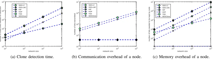
5) We provide a thorough evaluation of our proposed method considering different evaluation criteria, i.e., the clone detection probability and computation time of our algorithm when adopting our proposed speed-up methods. Moreover, we provide analytical and experimental comparisons of MDSClone with state-of-the-art clone detection methods. Our reported experimental results exhibit a perfect detection of clone nodes in the network, requiring a constant amount of memory and a reasonable communication overhead.
II. RELATEDWORK
In recent years, owing to the increasing interest in adopting WSNs in several applications, there has been a surge of interest in providing WSN-specific security solutions, amongst which clone attack detection has attracted significant attention. In this section, we review the clone detection methods that are most closely related to our work, and clarify the difference between our proposal and the existing related work.
Researchers [7], [8] have proposed several classifications for clone detection approaches based on the required information (i.e., location-based or location-independent), detection methods (i.e., centralized, distributed, or partially distributed), and supporting network type (i.e., mobile or static networks). Our proposed MDSClone approach falls in the category of location-independent centralized methods supporting hybrid (both static and mobile) networks. We believe that the centralized nature of MDSClone is not a drawback, considering the emerging municipality-scale IoT networking technologies such as NarrowBand-Internet of Things (NB-IoT) [16] and LoRaWAN [17]. Indeed, a centralized security monitoring solution is perfectly inline with the hierarchical architecture fostered by such technologies, which are currently being supported by key players, including among others Cisco and Orange. For instance, the current LoRaWAN deployment being developed in the city of Rome concentrates all IoT sensor traffic collected by several tens of radio stations spread across the whole of the Rome municipality and relevant neighbors in a (logically) single centralized network server, which therefore appears to be a natural candidate to further host anomaly detection approaches such as MDSClone.
In the case of static networks, a popular approach for detecting clones iswitness finding. In essence, the idea behind witness finding is that the existence of clones must lead to location conflicts. More specifically, each node ucollects the location information, L(v), of its neighboring nodes, e.g.,v, and sends the collected location claims hv, L(v)i to some selected nodes. Nodes receiving two location claims with the same IDv, but with two distinct locations, will serve aswitness nodes, and witness the location conflict. The witness finding strategy not only detects the existence of clones, but also identifies the clone IDs.
A network-wide broadcast is the simplest way to find a witness, but this incurs a prohibitive communication cost. In [18], the authors proposed two approaches, randomized multicast (RM) and line-selected multicast (LSM), in order to reduce the communication costs of network-wide broadcasts. Two other approaches proposed in [19], i.e., single deterministic cell (SDC) and parallel multiple probabilistic cells (P-MPC), share the same spirit as RM and LSM. However, SDC and P-MPC are only efficient when the network is partitioned into cells. Compared with the aforementioned approaches, the protocol proposed in [20], i.e., the randomized, efficient, and distributed (RED) protocol, provides an almost-perfect guarantee of clone detection. RED utilizes a special centralized broadcasting device, such as a satellite and UAV, in order to periodically broadcast the node IDs responsible for detecting particular conflicting location claims. In another study, Zhang et al. [21] proposed four clone detection methods that take advantage of double ruling and the Bloom filter. Recently, Dong et al. [22] proposed the low-storage clone detection (LSCD) method, taking into account the memory requirements and residual energies of nodes. An inherent weakness among all of the witness finding-based approaches is the assumption of the knowledge of location information available for each node. A couple of solutions take alternative approaches to detect clones, such as the social fingerprint [23], predistributed keys [24], and random clustering [25] methods.
In the case of mobile sensor networks, by using a simple challenge-and-response strategy, XED [11] presents the first distributed clone detection method for mobile networks. However, it is vulnerable to collusions of the cloned nodes. EDD [11], [12] is a distributed clone detection method based on the discrepancy between the distributions of the numbers of encounters with clone and ordinary nodes. In [26], a base station (BS) collects the geographical positions of nodes, looking for a clone moving with a speed exceeding the pre-configured speed limit. In [5], [13], the same idea is employed, but the ordinary nodes play the role filled by the BS in [26].
node will be controlled by clones. Therefore, if clones adopt the above evasion strategy, then only the mobile nodes (rather than both static and mobile nodes) will be able to detect clones, reducing the probability of clone detection. On the other hand, the detection effectiveness of TDD, SDD-LC, and SDD-LWC partly relies on whether each node encounters a particular node too many times (similarly to EDD). As a consequence, if the clones adopt the above-mentioned evasion strategy, then the detection capabilities of the TDD, SDD-LC, and SDD-LWC methods will also be degraded. In addition, the HIP-HOP approach detects clones based on the fact that if two witness nodes are either one-hop or two-hop neighbors, then either the witness nodes or the node connecting two witness nodes will find the location conflict of clones. However, if witness nodes far away from each other happen to both be static, then they have no chance of being either one-hop or two-hop neighbors, thus reducing the probability of clone detection.
In summary, the existing clone detection methods devised for static networks cannot be applied to scenarios where node mobility would destroy the neighborhood and distance relations among the nodes. On the other hand, as mentioned above, the adoption of most of the mobile clone detection methods to hybrid networks results in a degradation of the clone detection probability. Therefore, in order to deal with clones in IoT environments, we need to provide a method that is “particularly” designed for hybrid networks, and does not rely on any assumption regarding the mobility pattern, if any. In addition, prior solutions largely rely on the assumption that each node is aware of its geographical position. However, as explained in Section I, this is not the case for IoT devices. As a consequence, the existing clone detection methods are not applicable to IoT environments. Table I presents a comparison between MDSClone and the other existing clone detection schemes, in terms of the communication and memory overhead, required information, and network type.
III. SYSTEMMODEL
In this section, we describe our considered network model and assumptions (Section III-A), as well as the attack model (Section III-B). Table II presents the list of employed notations.
A. Network Model
We consider an IoT network as a hybrid network consisting of two main entities: 1) n static and mobile nodes with unique IDs [29]: ID ∈ {1, . . . , n}; and 2) a base station (BS). Each IoT device periodically measures its distance with its neighboring nodes, and sends the information to the BS. In our system model, the BS is in charge of executing our proposed MDSClone algorithm and locating the “clones” (for a definition please refer to Section III-B) in the network. In particular, the BS periodically receives neighboring information for each node in the network, and constructs a location map (based only on the information received from the nodes) in order to detect clones (we explain the details of the MDSClone algorithm in Section V-A). The BS executes MDSClone offline, and each generated location map is dedicated to a snapshot of the network at timet. The main idea in our proposed method is that at time t, a nodex cannot have two different sets of neighbors, which means that xcannot be in two different locations of the network at time t. In our network model, we make the following assumptions:
• We assume that nodes are not “necessarily” aware of their exact geographical position. This assumption is based on the following two factors explained in the existing literature: i) As explained in [9], using GPS is costly in terms of energy and the requirements for extra hardware, and ii) researchers [30] believe that GPS-based positioning is not efficient in indoor scenarios. Therefore, we assume that some nodes (e.g., smartphones) may be GPS-enabled, and others (e.g., home appliances) may not. Hence, our proposed method does not rely on geographical positions of nodes. This assumption is to address the first challenge that we mentioned in the “Problem Statement” Section, i.e., lack of accurate geographical position information of the devices. • We assume that mobile nodes are moving without any
particular mobility pattern. This assumption makes our network model more realistic, because the mobility patterns of nodes (e.g., wearable sensors) in IoT scenarios are unpredictable, as explained in [10]. We make this assumption to consider the second challenge that we mentioned in the the “Problem Statement” Section, i.e., IoT networks are hybrid networks composed of both static and mobile devices without a priori mobility pattern.
• We also assume that IoT devices are capable of enacting short-range device-to-device communication (as explained in [10]). Therefore, each node can measure its distance from its neighboring nodes via radio signal strength (RSS) or time of arrival (ToA) (as comprehensively discussed in [9], [30]). Although the estimated distances are not perfectly accurate, they are sufficient for our approach. We make this assumption, as in our proposed approach, each IoT device should periodically measure its distance with its neighboring nodes and send to the BS.
• We assume that the BS knows the geographic positions of IoT devices at the very beginning (only during the initialization of the network). However, after the network deployment, the BS is no longer aware of the positions of the devices. We make this assumption because the setup and deployment of IoT devices in the network are generally performed by the network designer, and so it is reasonable to adopt such an assumption. This assumption helps the BS in detecting and locating the clone nodes by comparing the constructed location map by the information received from the nodes and the original network map.
• We also assume that there exists a loose time synchronization between the nodes1, and the network
operation time is divided into time intervals, each of which has the same length. These assumptions are in line with other clone detection methods, e.g., [5], [31]. We make this assumption since each generated location map is dedicated to a snapshot of the network at timet. • We assume that the exchanged messages are digitally
signed2 before being sent out, unless stated otherwise.
We have studied the practicality and efficiency of such operations in [32], [33]. We make this assumption to ensure the confidentiality and accuracy of the exchanged neighboring information, based on which the location
1Because IoT devices are usually assumed to have an Internet connection,
relying on the network time protocol (NTP) could be one solution to achieve a loose time synchronization among nodes.
2Similar to [18], [31], we can assume that a light weight ID-based public
TABLE I: Comparison between different clone detection schemes.
Schemes Communication cost Memory cost Location-based Network type
RM[18] O(n2) O(√n) Yes Static
LSM[18] O(n√n) O(√n) Yes Static
Social Finerprint[23] O(n√n) O(1) No Static
CC-MEM[21] O(n√n) N/A Yes Static
RAWL & TRAWL[27] O(n√nlogn) O(√nlogn) Yes Static
SDC & P-MPC[19] O(ndp√n) +O(s) O(t) Yes Static
RED[20] O(nwdp√n) O(wdp) Yes Static
ERCD[28] O(n√n) O(1) Yes Static
LSCD[22] O(n√n) O(dl/re) Yes Static
TDD[13] O(√n) O(n) Yes Mobile
SDD-LC & SDD-LWC[13] O(1) O(n) Yes Mobile
SPRT[26] O(√n) O(1) Yes Mobile
XED[11] O(1) O(n) No Mobile
EDD[11] O(1) O(1) Yes Mobile
HIP-HOP[5] O(n) O(1) Yes Mobile
MDSClone(proposed approach) O(n√n) O(1) No Hybrid n: number of nodes,w: number of witnesses generated by a neighboring node,d: average node degree,p: probability of forwarding a message,t: number of witness nodes that store a location claim,c: number of nodes in a cell,l: length of a witness path,r: transmission range of a node.
TABLE II: List of notations used in this paper.
Notation Description BS Base station.
n Number of nodes in the network. di,j Distance between nodesiandj.
D∈Rn×n Distance matrix (distance between each pair of
nodes).
X∈Rn×p Coordinate matrix (ground truth node map).
B∈Rn×n Inner product matrix.
X0
t∈Rn×p Reconstructed coordinate matrix (node map).
λ Distortion threshold.
Lt Neighbor-distance information received by the BS at
t-th time interval.
D(λ,Lt, Xt0,L¯t)
Distortion function.
M(Lt,Lt−1) Localization function.
`t
i Location of nodeiat time intervalt(a column
vector).
map will be generated.
It is worth mentioning that all of our assumptions are consistent with the existing literature, and there are several real-world applications supporting our assumptions. Examples of IoT networks are the smart home and smart city, where a large number of static and mobile devices with unique IDs collaborate to provide a better quality of life for humans. For example, the Samsung SmartThings Home Monitoring Kit3 provides a hybrid network in which several static nodes (e.g., smart fridges, smart lamps, or smart thermostats) and mobile nodes (e.g., smartphones) can connect to each other. This kit comes with a hub and several smart things that could connect to each other and the hub through single-hop or multi-hop communication (using the repeaters that exist in the kit)4.
Another example is the Cisco Smart City5, in which there
are static nodes (e.g., traffic lights) and mobile nodes (e.g., Internet-connected cars). Moreover, several EU projects (e.g., the EU H2020 Wise-IoT project6or Santander city in the UK7) are examples of real-world heterogeneous IoT environments.
3https://www.youtube.com/watch?v=XQfAqlc7Vj8
4https://blog.smartthings.com/iot101/a-guide-to-wireless-range-repeaters/ 5https://www.youtube.com/watch?v=x6WfZlETbx4
6http://wise-iot.eu/en/home/ 7http://www.smartsantander.eu/
B. Attack Model
IoT devices are usually considered not to be tamper-resistant [34]. In other words, the stored security credentials can all be extracted in the case of a device bein compromised. Moreover, the adversary can compromise a device immediately after the node deployment. No secure bootstrapping time is available. Thus, the adversary can access all of the legitimate credentials of the compromised devices. In this paper, we consider an adversary that is capable of performing “clone attack”, meaning that they are able to fabricate compromised devices and store the legitimate credentials from the compromised devices inside several fabricated devices, which is (consistent with related work on clone detection such as [11]). A compromised node, as well as the fabricated nodes that have the same ID and credentials as the compromised node, are called clones. Clones can communicate and collude with each other, attempting to subvert the detection functionality in a stealthy manner. It should be noted that we only consider cloning attacks, and we assume there is no concurrent “node compromise” attack, meaning that no other nodes (beyond the clones) act in a malicious manner.
[image:5.612.50.301.270.435.2]Rather than a generic clone model consisting of s clone groups, each of which contain at most z clones, we consider a simplified clone model, similar to [11]. In our model, there is only one clone group, with exactly two clones having the same ID. The clone ID refers to the ID of two clones in a specific clone group, unless stated otherwise. The use of such a simplified model is to ease the presentation of our main idea, while our method can naturally be applied to a generic clone model without compromising the security.
IV. PRELIMINARIES
Before introducing our proposed clone detection method, we provide a brief background regarding MDS in Section IV-A, which serves as the foundation of our approach. A localization method using MDS that we describe in Section IV-B, called MDS-MAP, provides a core subroutine in our scheme.
A. Multidimensional Scaling
Multidimensional scaling (MDS) [14] is a hyperspace embedding technique, through which pairwise distances are fit into a set of coordinates with the preservation of distance restrictions. More concretely, MDS takes a distance matrix D as input, which is formed from the distances between all pairs of nodes. The output of MDS is a set of coordinates created using only D. The first step is to calculate an inner product matrix B = CAC, which satisfies the relation B = CAC =XXT, where C =I− 1
nEE
T,A = −1
2D
2,
I is an identity matrix, E is a column vector composed of 1’s, and X is a coordinate matrix with each row being a p-dimensional coordinate. One can easily observe that B is a real-valued and symmetric matrix, and hence we can apply orthogonal diagonalization to B to obtain
B=QM QT, (1)
where M = diag(µ1, . . . , µn), each µi(i ∈ {1, ..., n}) is
an eigenvalue of B, and Q = [q1· · ·qn] is composed of the
corresponding orthogonal eigenvectors. Owing to the fact that B =XXT, we can obtain the reconstructed coordinate matrix
X0 by calculating
X0 = [q1 · · · qp]
√
µ1
. .. √ µp
. (2)
However, the coordinate matrixX0reconstructed by MDS is not necessarily identical to X. In essence, X0 is only guaranteed to preserve the pairwise distancesD, but is subject to translations (shifts), rotations, and reflections. In other words, X and X0, where we write X 6=X0, can both act as the reconstructed coordinate matrix if X and X0 can induce the same D.
B. Localization via MDS
Given a network, MDS-MAP [15] is a localization algorithm executed by the BS. In particular, MDS-MAP takes a subset of pairwise distances of the nodes as input, and generates the coordinates of the nodes in the network. The difference between the ordinary MDS and MDS-MAP lies in the fact that the calculation of MDS assumes that the BS
has the knowledge of all pairwise distances. However, this assumption is not realistic, particularly in wireless networks. Thus, MDS-MAP combines the techniques of MDS and a shortest path calculation from graph theory to approximate the ordinary MDS. More specifically, in the case where nodes i and j are far away from each other and i cannot obtain a measured distance from j, the BS instead obtains an approximate di,j (i.e., the distance between i and j)
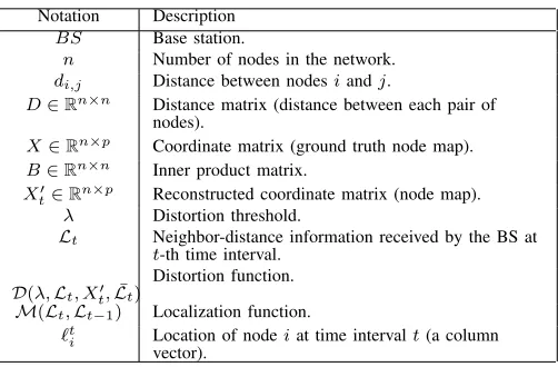
by calculating the corresponding shortest path. Using this approach, the BS can easily obtain all of the pairwise distances, although some of these are approximate. Next, the BS performs ordinary MDS on the pairwise distances to derive the coordinate matrix and accomplish the localization. Although the approximate distances comprising the input to MDS may cause a certain distortion in the reconstructed coordinates, Shang et al. [15] demonstrated the acceptable reconstruction accuracy of MDS-MAP. Figure 1 shows an illustrative example of the MDS-MAP process. In Figure 1a, each node measures its distance from its neighbors and reports this to the BS. Then, the BS uses the MDS-MAP reconstructed coordinates as the nodes’ positions to construct the network map, as shown in Figure 1b.
A B
C
D
E F
G
H I
J K
L
BS
(a) Nodes send their pairwise distances to the BS.
B J A
C
D
E F
G
H I
K
L
B J A
C
D
E F
G H
I K
L
BS
[image:6.612.317.562.299.432.2](b) BS uses MDS’s output to rebuild a map.
Fig. 1: An example of the MDS-MAP procedure.
V. PROPOSEDMETHOD
In this section, we describe MDSClone, our proposed method for clone detection. In particular, we explain the basic construction of MDSClone in detail in Section V-A. Then, in Section V-B we describe several improvements to our main construction to yield a more efficient clone detection algorithm. Note that although we mainly use MDS-MAP [15] to calculate the coordinates of IoT devices throughout the paper, we only use the term “MDS” in the remainder of the paper, for representational simplicity.
A. Main Construction of MDSClone
The idea behind our proposed MDS-based solution, MDSClone, is inspired by the following observation: When each node reports itsneighbor-distance information, consisting of its neighbor list along with the measured pairwise distances, to the BS, the BS can construct a node map8 via MDS
without the need to know the exact location information
8The terms “node map” and “coordinate matrix” are used interchangeably
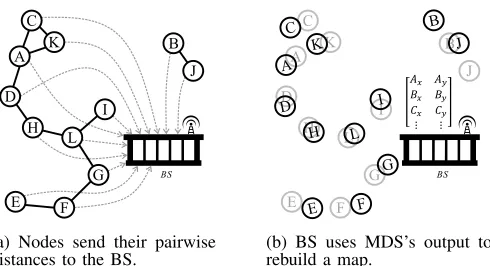
of the nodes. Note that the node map refers here to a set of coordinates of IoT devices, and corresponds to the coordinate matrix X in Section IV-A. In the case that no clones are present in the network, a coordinate matrix X0 will be generated such that the collected pairwise distances can be approximately preserved (i.e., each entry of the matrix D − D0 is close to 0, where D0 is the distance matrix calculated from X0). On the other hand, consider a network with a clone. From the BS’s perspective, if the information reported from devices collectively contains two nodes with the same ID but completely different neighbor lists, then the reconstructed node mapX0 will be distorted. More precisely, because two clones can be thought of as two identical nodes that simultaneously appear at two distant locations (e.g., node B in Figure 2a), at least one additional dimension is required in X0 to achieve distance preservation. Because the number pof dimensionalities should be a fixed and public parameter, or we may even restrict ourselves to two-dimensional MDS reconstruction (p = 2), it follows that a distortion in the reconstructed map is unavoidable (see Figure 2b). As a consequence, from the perspective of clone detection, the failure of MDS in constructing a node map that achieves distance preservation indicates the existence of clones in the network. To identify clones, the BS may execute MDS multiple times, excluding different node IDs. For example, if the MDS calculation for nodes {1, . . . , n} results in an erroneous node map, and the MDS calculation excluding node i (i.e., on nodes {1, . . . ,(i−1),(i+ 1), . . . , n}) achieves a perfect node map reconstruction, then nodeimust be a clone, because it caused the distortion in the MDS.
In what follows, we describethreemain design challenges that appear in adopting MDS for clone detection, and explain how MDSClone addresses these challenges.
• First, BS requires the pairwise distances of all the nodes in the network in order to run the MDS algorithm. However, such information is not available. Therefore, the first challenge is to enable the BS to perform the MDS calculation using only a “subset” of pairwise distances. The reason behind this challenge is that in an IoT network, each IoT device can only estimate its distance from its neighboring nodes, e.g., via RSS. Hence, the neighboring information reported to the BS does not include the pairwise distances of all nodes in the network. We address this challenge by using the shortest path between two nodes in order to approximately calculate the Euclidean distance between them (inspired by MDS-MAP [15]).
• The second challenge is to design a localization function (i.e.,M(Lt,Lt−1)) in order to “locate” the clones in the network. The reason behind this challenge is that the node map reconstructed by the BS is not necessarily identical to the real positions of nodes (although the pairwise distances are guaranteed to be preserved). In order to address this challenge, we consider two different cases (i.e., the existence of anchor nodes and lack of anchor nodes), as we explain in Section V-A1c.
• The third challenge is the computational overhead imposed on the BS. The reason behind this challenge is that the BS must perform the MDS calculations iteratively in order to find clones. In particular, the BS has to perform, on average, O(nc)rounds of MDS calculations
(where n is the number of nodes in the network and c is the number of clones). We address this challenge by proposing two strategies in MDSClone (as explained
in Section V-B): (i) reducing the MDS computational overhead, and (ii) performing the MDS calculation on several server-side devices in a parallelmanner.
B’
(a) Two nodes with the same ID (nodes B andB’).
B’
[image:7.612.330.594.107.225.2](b) Distorted reconstructed node map.
Fig. 2: An example IoT network with node B as a clone (we named the clone nodes as B andB’for clarification).
1) Detailed Description of MDSClone
The algorithmic description of MDSClone is presented in Algorithm 1. As can be seen, BS is in charge of running the algorithm and recognizing the existence of a clone in the network. Each nodeiin the network discovers its neighboring nodes Ni, measures the distance {(di,j)}j∈Ni with each
of its neighboring nodes, and sends this neighbor-distance information ht, i,{(j, di,j)}j∈Nii to the BS (comprising the
input of Algorithm 1) at time t9. Here, the message ht, i,{(j, di,j)}j∈Niican be thought as a star-shaped subgraph
whose nodes are Ni ∪ {i}. The purpose of this step is for
the BS to collect the subset of pairwise distances, similar to the case in MDS. With the neighbor-distance information of the nodes and a pre-defined distortion threshold (which we will explain in Section V-A1a) as input, the BS periodically executes Algorithm 1.
We assume that the BS maintains a table L for storing the received neighbor-distance information. After receiving the messages {ht, i,{(j, di,j)}j∈Nii}i=1,...,n, the BS stores
the star-shape subgraph induced from ht, i,{(j, di,j)}j∈Nii
at time t in the t-th row, Lt, of the table L (steps 2
and 3 of Algorithm 1). Hence, the t-th entry Lt of the
table L consists of the neighbor-distance information sent by all the nodes at time t. Then, the BS has to perform MDS over Lt to check whether there are clones present
(step 4 of Algorithm 1). More specifically, if the Boolean distortion function D(λ,Lt, Xt0,L¯t), that measures the
dissimilarity between pairwise distances from Lt and Xt0
(we will explain this function in Section V-A1b) returns true (step 5 of the Algorithm 1), this indicates a significant distortion in the reconstructed node map. In this case, the BS recognizes clones by applying MDS iteratively to Lt\
(π1,{(j, dπ1,j)}j∈Nπ1). . .(πρ,{(j, dπρ,j)}j∈Nπρ)
(steps 6∼8 of Algorithm 1). In essence, this is equivalent to applying MDS over the induced subgraph. During the MDS calculations, after the BS has determined a reconstructed node map whose pairwise distances are not consistent with the collected pairwise distances (step 9 of Algorithm 1), the
9Throughout this paper, the notation for timetis sometimes omitted (e.g.,
the setNt
i of neighboring nodes and the distancedti,j betweeniandj at
timetare abbreviated asNianddi,j, respectively) without ambiguity, when
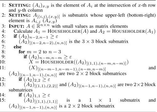
Algorithm 1 MDSClone performed by the BS.
1: Input:ht, i,{(j, di,j)}j∈Nii: neighbor-distance information received from nodei;λ: distortion threshold. 2: Ifreceiving{ht, i,{(j, di,j)}j∈Nii}i=1,...,n
3: UpdateLtby calculatingLt= (i,{(j, di,j)}j∈Ni) 4: Xt0=MDS(Lt)
5: IfD(λ,Lt, Xt0,∅) =True
6: Forρ= 1. . . n
7: Fordistinct tuplesn(π1,{(j, dπ1,j)}j∈Nπ1). . .(πρ,{(j, dπρ,j)}j∈Nπρ)
o
π1,...,πρ∈{1,...,n}
8: Xt0=MDS
Lt\
n
(π1,{(j, dπ1,j)}j∈Nπ1). . .(πρ,{(j, dπρ,j)}j∈Nπρ)
o
π1,...,πρ∈{1,...,n}
9: IfD(λ,Lt, X0t,
n
(π1,{(j, dπ1,j)}j∈Nπ1). . .(πρ,{(j, dπρ,j)}j∈Nπρ)
o
π1,...,πρ∈{1,...,n}) =False
10: Nodesπ1,. . .,πρare identified as clones
11: CalculateM(Lt,Lt−1)to locate clonesπ1,. . .,πρ
BS notices that the excluded nodes in the current calculation are clones (step 10 of Algorithm 1). By calculating the localization function M(Lt,Lt−1), the BS identifies and locates the clones (step 11 of Algorithm 1).
a) Choice of λ: The distortion threshold, λ, controls the trade-off between the tolerance of the MDS reconstruction error, the computational burden on the BS, and the capability of MDSClone to identify clones. In essence, in the case of a small λ value, MDS reconstruction inaccuracies may be regarded as clones, which leads to repeated MDS calculations in order to find these clones. On the other hand, an inappropriately large λ value may result in the misdetection of clones. As can be seen, determining a suitable λ value is important, and in fact a high sensitivity of the MDS reconstruction accuracy leads to a greater capability in identifying clones. In order to address these challenges, in the following we propose a data-driven method to determine an appropriate λ value. Hence, there will be rare cases in which clones could successfully evade detection owing to an inappropriate selection ofλ.
Owing to the fact that IoT devices are all owned by the IoT network owner, all the characteristics of the IoT devices, such as their radio ranges, are available to the network owner. Therefore, the network owner is able to virtually deploy IoT devices in a random manner, and then perform the MDSClone calculation on the virtual deployment. Here, we make two observations. First, even in the virtual deployment without clones, the distance matrixDderived directly fromLtwill be
slightly different from the distance matrixD0derived from the MDS-MAP reconstruction result. Second, in the presence of clones in the network, the discrepancy betweenDandD0must be significant, because clones are usually not close to each other, in order to have a more negative impact on the network. As a result, to determine a suitable λ, the network owner sets upxvirtual deployments without clones, and chooses the maximum discrepancy value among the xdiscrepancy values as λ, wherexis a sufficiently large value. More precisely, let A(D0, D)i be given byA(D0, D) =
P
i<j(d
0
i,j−di,j)2
1+···+(n−1) , derived in the i-th virtual deployment (a more detailed description of A(D0, D) can be found in Section V-A1b). The distortion threshold λ is set as the maximum distortion10, i.e., λ =
max{A(D0, D)1, . . . ,A(D0, D)x}.
10In the execution of step 9 of Algorithm 1,DandD0are not necessarily
of dimensionsn×n. Thus, one can calculate differentλ’s for the calculation ofD(λ,Lt, Xt0,L¯t)onDandD0of different sizes. This could constitute a
natural extension of the idea behind the calculation ofλhere. For the sake of notational simplicity, we omit the detailed explanation of such a fine-grained control ofλin this paper.
b) Construction ofD(λ,Lt, Xt0,L¯t): Similar toλ, the
distortion function, i.e., D(λ,Lt, Xt0,L¯t), has direct impact
on the trade-off between the tolerance of MDS reconstruction error, computation burden on the BS, and capability of MDSClone in identifying the clones, but the corresponding construction is still unclear.
Here, we propose an algorithm as an implementation of D(λ,Lt, Xt0,L¯t). More specifically, the algorithm takes as
input a distortion thresholdλ, the received neighbor-distance information Lt, and the reconstructed node map Xt0, and
outputs an indication of whether the pairwise distances from Ltare inconsistent with the ones fromXt0. In particular, with
the shortest path as an approximation, the BS can calculate pairwise distances D = {di,j}i,j∈{1,...,n} from Lt \ L¯t.
X0
t can also be used to generate estimated distance matrix
D0 ={d0
i,j}i,j∈{1,...,n}. Hence,D(λ,Lt, Xt0,L¯t) returns true
(significant inconsistency betweenDandD0, indicating clone
existence) if A(D0, D) =
P
i<j(d
0
i,j−di,j)2
1+···+(n−1) ≥ λ and false otherwise. Note that A(D0, D) here is defined based on the least square error criterion, while, it is possible to adopt other error metrics.
c) Construction ofM(Lt,Lt−1): After identifying the clones, one option is to announce and revoke clone IDs. In this case, since the nodes physically remain in the network, the attacker might use them in order to conduct other clone attacks or other types of attack, such as blackhole or jamming attacks. Another option is to locate clones and then physically remove them or use one of the existing attestation techniques in the literature (such as [35]). In order to protect the network against further attacks, the latter case is preferable. In this latter case, we need to develop techniques for locating clones in the network, and for that matter we introduce the localization functionM(Lt,Lt−1), which we detail in the following.
We consider two constructions for M(Lt,Lt−1): (i) Anchor case: a network having at least two static nodes, (ii) No anchor case: without having such restriction. The idea behind the two constructions of M(Lt,Lt−1) is node alignment: once the real location of nodes at the previous time are known and the alignment between Lt and Lt−1 can be made, we can easily infer the real locations at the current time. In what follows, we explain the considered two scenarios.
Consider the case where the BS applies MDS to nodes 1, . . . , n. The transformation matrix can also be applied only to a subset 1, . . . , s, where1, . . . , s are static nodes, without loss of generality. In other words, if X = [X1TX2T]T and X0 = [X0T
1 X20T]T, then X10T = X1P and X20T = X2P. A closer look to the currently used MDS reveals that the MDS works in a restricted form; the mean of reconstructed coordinates of the MDS result will always be shifted to [0 0], in the two-dimensional case. This eliminates the need for handling the translation operation, because one can shift the locations at the previous time to be centered at [0 0], perform the node alignment, and perform the reverse shift on aligned locations. In this sense, we can therefore take care of the rotation and reflection operations only. Since the MDS is primarily featured by an orthogonal diagonalization (see Section IV-A), we simply find an orthogonal matrix to solve the problem. In particular, we look for an orthogonal matrix P such that X0 =XP with the property of
X0X0T =XP(XP)T =XP PTXT =XXT =B. (3)
To find such aP, we randomly choose two static nodes from 1, . . . , s, and their corresponding reconstructed coordinates. The transformation matrixP can be calculated by considering
the relation between two chosen nodes,
x01 y10 x02 y
0
2
= X0 =
XP =x1 y1 x2 y2
P, and can be derived as follows,
P = 1
x2y1−x1y2
x02y1−x
0
1y2 y
0
2y1−y
0
1y2
x02x1−x
0
1x2 y
0
1x2−y
0
2x1
. (4)
Note that the determinant of P, det(P), may determine the operations applied to nodes. Note also that an odd number of reflections implies det(P) = 1, while the other cases (e.g., only rotation or an even number of reflections) imply det(P) =−1. After obtainingP, we perform node alignment to keep track of the clone movement. In particular, the reconstructed coordinates will be transformed via P to be consistent with the coordinates at the previous time.
No Anchor Case. In this scenario, we do not have anchors and instead seek a construction of M(Lt,Lt−1) for mapping two sets of points with the guarantee of minimal node-wise discrepancy. The algorithm for the node alignment is inspired by the problem of point set registration. The point set registration [36] has been widely used in computer vision community for finding a spatial transformation that aligns two sets of points. In particular, the point set registration merges two data sets into a globally consistent model by mapping a new measurement to a known data set. The Iterative Closest Point (ICP) algorithm [37] is the most straightforward way for minimizing the difference between two clouds of points. However, ICP works only in the case of a rigid registration (or say, rigid transformation), which typically consists of translation and rotation. The point set registration can also be used in our case where the nodes location at the previous time are mapped to the ones at the current time. However, our problem can be thought as a variant of the conventional point set registration. The differences are stated below:
• While the size of two sets of points in the conventional point set registration problem are allowed to be different, in our case they are guaranteed to be the same.
• While one set of points will be deterministically transformed from another set, in our case due to the consideration of node mobility, we may consider
the option of either imperfect transformation or noisy transformation.
Moreover, the MDS-reconstructed node map is subject to not only translation and rotation but also reflection operations, as shown in Section IV-A. Thus, inspired by the robust affine transformation consisting of a richer set of transformations including translation, rotation, and reflection, we resort to affine variant of ICP, affine ICP, to find the transformation matrix P between {`t1−1, . . . , `t−1
n } and {`t1, . . . , `tn}, where
`ti−1and`t
iare the coordinate of thei-th node at(t−1)-th time
andt-th time, respectively, with Xt−1 = [`t1−1· · ·`
t−1
n ]T and
Xt = [`t1· · ·`tn]T being the coordinate matrices at (t−1)-th
time and t-th time, respectively.
Since affine transformation is a richer set of transformations compared to the three transformations required in our context, our problem can still be recasted as the affine registration of two two-dimensional point sets. More formally, based on the least-square error criterion, the affine registration between two point sets can be formulated as
min
P,j∈{1,...,n}
n X
i=1
||P(`ti−1)−`tj||2 2
!
. (5)
However, the transformation P in Equation (5) is too vague; it needs to be expressed explicitly so as to simplify the objective function in Equation (5). With the fact that the affine transformationP can be decomposed into an invertible matrix Φ together with a translation vector s, Equation (5) can be rewritten as
min Φ,s,j∈{1,...,n}
n X
i=1
||(Φ`ti−1+s)−`tj||22
!
. (6)
Note that the presence of anchors eliminates the need of handling coordinate shift but the lack of anchors does not. Furthermore, an invertible real-valued matrix Φ can be decomposed via singular value decomposition (SVD) into Φ = U SVT, where U and V are orthogonal matrices and S is a diagonal matrix with singular values. Because VT is orthogonal matrix, we define the rotation matrix R = VT.
After all, the objective function in Equation (6) can be rewritten as
min
U,S,R,s,j∈{1,...,n}
n X
i=1
||(U SR`ti−1+s)−`tj||2 2
!
. (7)
Recall that an affine transformation is a combination of a series of basic transformations, such as translation, rotation, and reflection. In Equation (7), U and R represent reflection and rotation matrices, respectively, while S is a scale matrix. Though U and R are orthogonal matrices, the collection of nodes does not scale differently in our consideration. Considering the above constraints, the unconstrained optimization in Equation (7) can be transformed to a constrained optimization,
min
U,R,s,j∈{1,...,n}
n X
i=1
||(U R`ti−1+s)−`tj||2 2
!
s.t. UTU =I, det(U) = 1
RTR=I, det(R) = 1
Inspired by robust affine ICP [36], the optimization in Equation (8) can be solved in the iterative algorithm shown in Algorithm 2. Algorithm 2 outputs rotation matrices Uk,
Rk, and translation vector sk. More specifically, given the
(k−1)-th transformations (Uk−1, Rk−1, sk−1), the step 3 of Algorithm 2 aims to establish the correspondence of point sets:
ck(i) = argmin j∈{1,...,n}
||(Uk−1Rk−1`it−1+sk−1)−`tj||
2 2
, (9)
where i= 1, . . . , n. Note that, step 3 of Algorithm 2 can be solved by methods such as k-d tree [38] and nearest point search based on Delaunay tessellation [39]. Given the found correspondenceck(i), step 5 of Algorithm 2 computes thek-th
transformations(Uk, Rk, sk):
(Uk, Rk, sk) = argmin U∈L(2),R∈L(2),s∈R2
n
X
i=1
||U R`ti−1+s−`t i||22
!
,
(10)
where L(2) = {Υ ∈ R2×2|ΥTΥ = I2,det(Υ) = 1} denotes an orthogonal group consist of a set of real 2 × 2 orthogonal matrices. Considering the Taylor series of exponential mappings on Uk, Rk ∈ L(2), step 5 of
Algorithm 2 can be formulated and solved using quadratic programming.
Algorithm 2 Node alignment based on affine ICP.
1: INPUT:kis initialized as0;U0,R0, ands0are randomly chosen;is the considered threshold.
2: Repeat
3: Compute the correspondence (Equation (9)) by using Uk−1, Rk−1, sk−1
4: Compute the error function k(U, R, s) =
1
n
Pn
i=1||(Uk−1Rk−1`ti+sk−1)−`tj−1||22
5: Compute thek-th transformation(Uk, Rk, tk)andk=k+ 1
6: Until |k(Uk, Rk, sk) −k−1(Uk−1, Rk−1, sk−1)| ≤ or k
reaches a predefined threshold
Lemma 1. Algorithm 2 converges monotonically to a local minimum, with respect to the mean squared distance from any given initial parameters.
Algorithm 2 shares the same spirit as robust affine ICP [36]. Nevertheless, due to its similarity to robust affine ICP and the lack of space, we omit the formal proof of Lemma 1 here.
B. Techniques for Efficiency Improvement of MDSClone
As we explained in Section V-A, the BS should execute the Algorithm 1 in order to check if the network is under clone attack, and in case of having clones, BS should execute MDS function (steps 7 to 10 of Algorithm 1) multiple times to identify the clone IDs. In such situation, BS has to perform, on average, O(nc) rounds of MDS calculations11 to find the
clones, provided thatcclones exist in the network. Though the MDS computation is very fast, the iterative calculation of MDS may still impose a huge computation overhead on the BS. For example, the execution of the MDS on a matrix of dimension 104×104takes approximately two minutes. In the case of only
11In the extreme case, assume that there is one clone group consists of
c clones in the network. Since these c clones share the same ID (where ID∈ {1, . . . , n}), the MDSClone has to perform the MDS calculation for O(n)times (on average n2 times) to identify the clone ID. Consider another extreme case, wherecclone groups exist in the network. Since the BS has no knowledge on the number of clones (i.e.,c), the BS has to scan every possible combination of clone IDs, leading toO(n) +O(n2) +· · ·+O(nc) =O(nc) times of MDS calculations, whereO(ni)comes with n
i
possibilities of one clone ID (wherei= 1. . . c).
one clone in a network of 104 IoT devices, the BS needs to perform the MDS, on average,5×103times, which requires hours or even days for detecting the clones. In what follows, in order to address this issue, we propose an improvement to the calculation of the MDS function. In particular, we show that the MDS calculation can be parallelized and offloaded on several powerful servers, or devices, each of which calculating one of the required iterations that results in speeding up the whole clone detection algorithm. We show that our proposal significantly reduces the computation load on the BS, leading to improved scalability and performance of the clone detection method. We provide detailed explanation of our improved implementation in the following.
1) Speeding Up the MDS Calculation
In general, a significant portion of computation overhead in the MDS calculation is incurred by computing eigenpairs. Here, the eigenpairs mean the pairs of eigenvalues and eigenvectors in Equation (1). In addition, obviously the computation load in the MDS is proportional to the number of nodes in the network. To ensure the scalability of MDSClone, with the observation that the inner product matrix B in our context is always real-valued and symmetric, we propose three techniques to improve the performance of the MDS calculation in MDSClone algorithm:
a) CIPMLO:aims at computing inner product matrix with less arithmetic operations.
b) TI:is using modified Householder transformation [40] to speed-up the calculation of eigenpairs.
c) SMEBM:is closely relevant toTI, and basically speeds-up TI.
Each of these three techniques leads to certain extent of the speed-up. Among them,CIPMLOandTIcan be executed individually, while SMEBM is useful only when it is used along withTI. We detail each of these three techniques in the following.
a) Computing Inner Product Matrix With Less Operations (CIPMLO): This technique, computes inner product matrix B with less arithmetic operations. Starting with a concrete example is helpful in giving an idea of how CIPMLO achieves the speed-up. Assume that we have a distance matrixD such that
D2=
"0 10 34 20
10 0 52 50 34 52 0 10 20 50 10 0
#
. (11)
We derive matrices C andA as follows,
C= 1
4
" 3 −1 −1 −1
−1 3 −1 −1 −1 −1 3 −1 −1 −1 −1 3
#
and
A=
" 0 −5 −17 −10
−5 0 −26 −25 −17 −26 0 −5
−10 −25 5 0
#
. (12)
We calculate the matrix Ω = C·A. A partial view of Ω is shown in the following,
Ω = 1 n
" 5 + 17 + 10 · · ·
−15 + 17 + 10 · · · 5−51 + 10 · · · 5 + 17−30 · · ·
#
. (13)
elements by using diagonal elements. In essence, the matrix Ωcan be represented in a more formal way as follows.
Ω =−1 n
D1 D2−nN1 D3−nN2 D4−nN3 D1−nN1 D2 D3−nN4 D4−nN5 D1−nN2 D2−nN4 D3 D4−nN6 D1−nN3 D2−nN5 D3−nN6 D4,
,
(14)
where Di =P n
j=1Aj,i and Nk is the non-diagonal element
in the lower triangular part ofA, with the elements ofAbeing re-numbered as 0
N1 0
N2 Nn . ..
..
. ... ... 0
Nn−1 N2n−3 Nn(n−1) 2 0 . (15)
Let Ωbe
Ω =−1 n
e1 e5 e9 e13
e2 e6 e10 e14 e3 e7 e11 e15 e4 e8 e12 e16
. (16)
Let S be −(e1+e5+e9+13). Recall that B= ΩC=CAC (see Section IV-A), we obtain
B= −1 n2
4e
1+S 4e5+S 4e9+S 4e13+S
..
. ... ... ...
. (17)
Similarly, we find that each element of B has relation with the sum of row elements ofΩ. In fact,Bcan be expressed in the following form,
B=−1 n2
ne1−R1 ne5−R1 ne9−R1 ne13−R1 ne2−R2 ne6−R2 ne10−R2 ne14−R2 ne3−R3 ne7−R3 ne11−R3 ne15−R3 ne4−R4 ne8−R4 ne12−R4 ne16−R4
,
(18)
where Ri is defined as Ri = S−nDi withS = P n i=1Di.
Then we prove thatRi is the sum of thei-th row of Ω.
Lemma 2. Ri is the sum of the i-th row ofΩ.
Proof. Ri=S−nDi=P n
i=1Di−nP
n
j=1Aj,i
=Pn j=1Ωi,j.
Then, we prove that ΩC calculated in our proposed procedures remains symmetric.
Lemma 3. ΩC is symmetric.
Proof. −n1ΩCi,j = −n1(nΩi,j−Ri) = −n1[n(Dj−nAi,j)−
(S−nDi)] =−n1[n(Di−nAj,i)−(S−nDj)] = −n1(nΩj,i−
Rj) = −n1ΩCj,i, where the first equality and second equality
are due to equations (18) and (14), respectively.
SinceB= ΩCis symmetric, we can calculate the elements of only upper or lower triangular part. In addition, we find that the upper triangular part of Bin Equation (18) is only dependent on the upper triangular part of Ω in Equation 16. In other words, we can calculate only a half of elements ofΩand then compute Bwith approximately half of the computing burden, compared to the original computation task. Such calculation of B is shown below.
B=− 1
n2ΩC =− 1
n2
"D1 D2−nN1 D3−nN2 D4−nN3
· D2 D3−nN4 D4−nN5
· · D3 D4−nN6
· · · D4
#
C
=− 1
n2
"ne1−R1 ne5−R1 ne9−R1 ne13−R1
· ne6−R2 ne10−R2 ne14−R2
· · ne11−R3 ne15−R3
· · · ne16−R4
#
. (19)
Note that the third equality is due to Equation (18).
b) Tridiagonalization Improvement (TI): Before calculating eigenvalue decomposition, the existing library for eigenvalue computation [41] introduces a pre-processing phase for computation reduction. In particular, when the matrix is symmetric, one can apply Householder transform to the input matrix and obtain a tridiagonal matrix. After that, the eigenvalue decomposition applies to derive the eigenvalues and eigenvectors. In our context, we focus only onB, which is naturally symmetric. Consequently, our second proposed technique,TI, to speed-up the MDS calculation is due to the performance improvement of matrix tridiagonalization.
Basically, TI achieves the speed-up because some matrix multiplications can be replaced by matrix additions and inner product calculations. We also start with how Householder transform works, to better illustrate the basic idea behind the design. Let A = A0 be a real-valued symmetric matrix of dimension n×n. We can reduce A to the tridiagonal form An−2 by iteratively using decomposition, Am =
PmAm−1Pm,m= 1. . .(n−2), where Pm=
hH
n−m 0
0 Im
i
is an orthogonal matrix withImbeing anm×midentity matrix
andHn−m being a Householder matrix defined as Hn−m=
In−m −2vn−mvnT−m. Here, vn−m = kxxn−m−σen−m
n−m−σen−mk is a
Householder vector, wherexn−mis a column vector composed
of the first n − m elements of the m-th column of A, σ=−sign(x•)kxn−mk is the length ofxwithx• being the last element of xn−m, en−m = (0, 0, . . . , 1)T is the last
standard basis vector of dimension(n−m)×1, andsign(x•) is defined as
sign(x•) =
n 1 ifx
1≥0
−1 ifx1<0 . (20)
Afterwards, we can generate the tridiagonal form of a given symmetric matrix. More concretely, consider the first iteration of Householder transformation ofA,
A=A0=
e1 e2 e3 e4
e2 e5 e6 e7 e3 e6 e8 e9 e4 e7 e9 e10
. (21)
Letxn−1=
he4
e7 e9
i
andvn−1= ˆ vn−1
sqrt, whereˆvn−1=
h e4
e7 (e9+σ)
i
andsqrt=pe2
4+e27+ (e9+σ)2. Then, we obtain
Hn−1=In−1− 2 sqrt2
e2
4 e4e7 e4(e9+σ) e7e4 e2
7 e7(e9+σ) (e9+σ)e4 (e9+σ)e7 (e9+σ)2
, (22) and P1=
1− 2e24
sqrt2
−2e4e7
sqrt2
−2e4(e9+σ)
sqrt2 0
−2e4e7
sqrt2 1−
2e27 sqrt2
−2e7(e9+σ)
sqrt2 0
−2e4(e9+σ)
sqrt2
−2e7(e9+σ)
sqrt2 1−
2(e9+σ)2
sqrt2 0
0 0 0 1
. (23)
As concrete examples, we list some elements ofP1A.
(P1A)1,1= (a)
z}|{
−2e4
(c)
z }| {
[e1e4+e2e7+e3(e9+σ)] sqrt2
| {z }
(a)
+ e1
|{z}
(b)
and(P1A)2,1= (a)
z}|{
−2e7
(c)
z }| {
[e1e4+e2e7+e3(e9+σ)] sqrt2
| {z }
(a)
+ e2
|{z}
(P1A)1,2= (a)
z}|{
−2e4
(d)
z }| {
[e2e4+e5e7+e6(e9+σ)] sqrt2
| {z }
(a)
+ e2
|{z}
(b)
and(P1A)2,2= (a)
z}|{
−2e7
(d)
z }| {
[e2e4+e5e7+e6(e9+σ]) sqrt2
| {z }
(a)
+ e5
|{z}
(b) . (25)
Before describing our approach based on modified Householder transformation, we highlight some observations from equations (24) and (25) as follows:
1) The elements with the same column have similar calculations.
2) All elements of P1A share some common operations (part (a)).
3) The elements in part (b) are the elements from matrix A.
4) The calculations in part (c) are the same, as well as the calculations in part (d).
5) The remaining parts, e4 ande7, are elements of vˆn−1.
TI mainly speeds-up some parts of the numerators of the elements inP1A(e.g., parts (c) and (d)), but for the time being, we only focus on part (c). Consideringe1e4+e2e7+e3(e9+σ), we recognize that this it is the inner product of ˆvT
n−1 and
[e1e2e3]T (i.e., part of matrixA). So,P1Acan be represented as
−2ˆvn−1(1)(X123)
sqrt2 +e1 −
2ˆvn−1(1)(X256)
sqrt2 +e2 · · · −2ˆvn−1(2)(X123)
sqrt2 +e2 −2ˆvn−sqrt1(2)(2X256)+e5 · · · −2ˆvn−1(3)(X123)
sqrt2 +e3 −
2ˆvn−1(3)(X256)
sqrt2 +e6 · · ·
e4 e7 · · ·
, (26)
Where vˆn−1(i) is the i-th element of ˆvn−1, X123 = ˆ
vT
n−1·[e1e2e3]T, and X256 = ˆvnT−1·[e2e5e6]T. Let Vr be the inner product ofvˆT
n−1 and[Ar,1Ar,2Ar,3]. Then,P1Acan be rewritten as
−2 sqrt2
hhˆv n−1
0
i
⊗([V1E V2E V3E V4E])
i
+A, (27)
where⊗denotes the element-wise multiplication andEis the vector of all1’s. By considering equations (23), (24), and (25), the same observations and procedures can also be applied to P1AP1(= A1) in order to obtain
A1(1,1)= S
|{z}
(e)
S
|{z}
(e) ˆ vn−1(1) ¯V1
| {z }
(f)
+ˆvn−1(1)V1+V1ˆvn−1(1)
+ e1
|{z}
(g) ,
(28)
A1(2,1)= S
|{z}
(e)
S
|{z}
(e) ˆ vn−1(2) ¯V1
| {z }
(f)
+ˆvn−1(2)V1+V2ˆvn−1(1)
+ e2
|{z}
(g) ,
(29)
whereS= sqrt−22 andV¯1= ˆvn−1(1)ˆvnT−1·[V1V2V3]
T
. We can see from equations (28) and (29) that for the elements of the same column in A1, they perform the same operations. For example, the multiplication withS (part (e)) and an inner product (part (f)) are common operations. We can also see
that the elements in part (g) are from matrix A. Let V¯i be
ˆ
vn−1(i)ˆvTn−1·[V1V2V3]
T
. Thus,A1 can be formulated as
A1=S2
hhˆv n−1
0
i
⊗[ ¯V1E V¯2E V¯3E 0E]
i + S h ˆ v 0 i V1 V2 V3 V4 T + V1 V2 V3 V4 h ˆ v 0 iT
+A.
(30)
Then, in the following lemma, we prove thatA1calculated in the above way is symmetric.
Lemma 4. A1 calculated in the above way is symmetric.
Proof. Letw= [ˆvn−1 0]T andW = [ ¯V1 V¯2 V¯3 0]
T
. A1(i,j) = S
2[w(i)W(j)] + S[w(i)V(j) + V(i)w(j)] +
Ai,j = S2[w(i)W(j)] + [w(i)V(j) + V(i)w(j)] =
S2[ˆv
n−1(i)ˆvn−1(j)(ˆvTn−1 · [V1 V2 V3]
T
)] =
ˆ
vn−1(i)ˆvn−1(j)ˆvnT−1 · [V1 V2 V3]
T
) =
S2[ˆvn−1(j)ˆvn−1(i)(ˆvTn−1 · [V1 V2 V3]
T
)] =
S2[w(j)W(i)] + [V(i)w(j) +w(i)V(j)] =S2[w(j)W(i)] + S[w(j)V(i) +V(j)w(i)] +Aj,i=A1(j,i).
According to the property of Householder transformation, after the first iteration,A1 can be expressed in the following form,
"∗ ∗ ∗ 0
∗ ∗ ∗ 0
∗ ∗ ∗ e
0 0 e d
#
. (31)
In the following lemma, we formally prove that the upper-right entry of A1 calculated in the above way is zero.
Lemma 5. The upper-right entry ofA1calculated in the above way is zero.
Proof. Assume (P1AP1)i,j = 0, where i ≤ j − 2 and
j≥n−2.
A1(i,j) = S[ˆvn−1(i)Vj] + Ai,j =
Shˆvn−1(i)
ˆ
vTn−1·[Aj,1 Aj,2 Aj,3]T
i
+ Ai,j =
S
ˆ
vn−1(i) ˆvn−1(1)Aj,1+ ˆvn−1(2)Aj,2+ ˆvn−1(3)Aj,3
+ Ai,j = S[Ai,j(A1,jAj,1+A2,jAj,2+ (A3,j+σ)Aj,3)] +
Ai,j = S
Ai,j A21,j+A
2
2,j+A
2
3,j+Aj,3σ
+ Ai,j =
S
Ai,j σ2+Aj,3σ
+Ai,j = S
Ai,j(−S−1)
+Ai,j =
−Ai,j+Ai,j = 0
We can see from Equation (30), Lemma 4, and Lemma 5 that the original matrix multiplications in Householder transform can be replaced by matrix additions and inner product calculations. The same observations and procedures can also be applied toA2,A3, and so on. As a consequence, we have the following corollary.
Corollary 1. The matrix multiplications involved in the calculation ofAi, wherei= 1. . .(n−2), can be replaced by
inner product and matrix addition calculations.
c) Searching for Meaningful Eigenpairs of Block Matrix (SMEBM): If the reconstructed coordinates are constrained to be two-dimensional, in fact, two largest eigenpairs suffice to reconstruct X0. Note that “meaningful eigenpairs” here refer to those eigenpairs that have impact on the coordinates of our interest. More specifically, as stated previously, we perform tridiagonalization and eigenvalue decomposition to derive X0. However, we observe that the two-dimensional node map is only affected by specific elements. As a result, the idea behind SMEBM is that we only calculate the entries that may affect the eigenpairs that have impact on the two-dimensional coordinates. One distinguishing feature ofSMEBMis that one may needn−2 iterations of calculations of A1, . . ., An−2 in TI, however, only two or three iterations inSMEBM are needed.
Given that all the elements ofA=A0 are very small, we observe from the tridiagonalized matrix that only some values of small block submatrix are meaningful. In particular, there are two forms of block submatrices.
Di Ei−1 0 · · · 0 Ei−1 . .. . .. . ..
. . .
0 . .. d3 e2 0 .
.
. . .. e2 d2 e1 0 · · · 0 e1 d1
and
di ei−1 0 · · · 0 ei−1 di−1 0 . ..
. . .
0 0 . .. 0 0 .
.
. . .. 0 d2 e1 0 · · · 0 e1 d1
. (32)
The first form is a3×3 block submatrix (see the former part of Equation (32)), containing two meaningful eigenvalues, where an eigenvalue is close to zero and will always be at the bottom-right corner. The second form is composed of two2×2 block submatrices (see the latter part of Equation (32)): they can be found in diagonal part of tridiagonalized matrix, an one of them is guaranteed to be at the bottom-right corner. Furthermore, in the case of two2×2block submatrices, each block submatrix contributes one meaningful eigenpairs. The reason why we can only focus on the block submatrix is that all the elements of tridiagonal matrix are close to zero except the elements of block submatrices.
To better illustrate the idea behindSMEBM, we start with a concrete example. Consider a 5×5 tridiagonal matrix in Equation (33) with a3×3block submatrix and “∗” elements between10−10 and10−16.
∗ ∗ 0 0 0
∗ ∗ ∗ 0 0
0 ∗ d3 e2 0 0 0 e2 d2 e1 0 0 0 e1 d1
. (33)
Since “∗” is very close to 10−10 and 10−16, we consider them to be zero. So, the eigenvalues of tridiagonal matrix ∆ can be easily extended to be the eigenvalues of matrix
h
O 0
0 ∆
i
by padding zero submatrix O. The above works only in the case where each element is sufficiently small. Nevertheless, a preprocessing step can be used to counteract the above problem. After calculating the inner product matrix, we scale it by calculating Bα, where α = Pn
d=1Bd,d +
Pn−1
r=1
Pn
c=r+1Br,c. Because of the above preprocessing on
the inner product matrix B, the eigenvalues calculated after the scaling, the values of µ0i, will not be the same as original ones, µi. However, µi can be recovered by calculating µi =
αµ0i, i = 1. . . n. Since we only need the block submatrix, we can reduce some steps when performing Householder transformation. In particular, for a 3×3 block submatrix, we just need to transform the inner product matrix twice. For two
2×2block submatrices, we need to transform the inner product matrix two or three times.
∗ ∗ ∗ ∗ + ∗ ∗ ∗ ∗ + ∗ ∗ ∗ ∗ + ∗ ∗ ∗ ∗ −
+ + + − d1
matrixA ⇒
∗ ∗ ∗ + 0
∗ ∗ ∗ + 0
∗ ∗ ∗ − 0
+ + − d2 e1 0 0 0 e1 d1
1st iteration (A1)
⇒
? ? ? 0 0
? ? ? 0 0
? ? d3 e2 0 0 0 e2 d2 e1 0 0 0 e1 d1
2nd iteration (A2)
(34)
From Equation (34), we can see that, after one iteration of Householder transformation, the positions with “+” mark will become zero, and the elements on the positions with “∗” mark will be changed because they are multiplied by Householder matrix. In the case of a 3×3 block submatrix, e2 must be greater than ε ≈ 10−10 and we do not need to compute the remaining parts with “?” mark. In the case of e2 ≤ ε, we deflate the matrix, resulting in the case of two 2 ×2 block submatrices. Basically, we check whether the diagonal elements are greater thanε. To search for the two2×2block submatrices, we have three different cases as follows.
1) One 2 × 2 block submatrix is at the bottom-right corner, while another is 1×1 block submatrix (or say, 2×2degenerated block submatrix with the bottom-right element being0) at the upper-left corner.
2) One2×2block submatrix is at the bottom-right corner, while another is2×2block submatrix at the upper-left corner.
3) One2×2block submatrix is at the bottom-right corner, while another is 2×2 block submatrix at the matrix diagonal part (but not at the upper-left corner).
elements with “” mark are≈0
di 0 0
≤ε 0 0
≤ε ≤ε 0 0 0 ≤ε d2 e1 0 0 0 e1 d1
first case (A2)
di ei−1 0 0
ei−1 di−1≥ε 0 0
≤ε ≤ε 0
0 0 ≤ε d2 e1 0 0 0 e1 d1
second case (square matrixA2)
? ? ? 0 0 ? ? ? 0 0 ? ? >ε≤ε 0 0 0 ≤ε d2 e1 0 0 0 e1 d1
third case (A2)
(35)
The above algorithm for 5×5 matrix can be extended to handle n×n matrix. Algorithm 3 searches for meaningful eigenpairs with the minimal number of iterations of Householder transformation. Two largest eigenpairs among three calculated eigenpairs in the case of a 3×3meaningful block submatrix or among four calculated eigenpairs in the case of two2×2meaningful block submatrices, in fact, suffice to reconstructX0.
VI. EXPERIMENTALANALYSIS