2016 International Conference on Artificial Intelligence: Techniques and Applications (AITA 2016) ISBN: 978-1-60595-389-2
A New Better-Fit Decision Features Selection
Method for C5.0 Decision Tree
Hong-wei YANG
*and Sheng-jie SUN
College of Information Science & Technology, Hainan University, No. 58, Renmin Avenue, Haikou City, Hainan Province, 570228, P.R. China.
*Corresponding author
Keywords: C5.0 decision tree, Better-fit decision features selection (BFDFS), Rubber woods classification from high resolution remote sensing image.
Abstract. C5.0 decision tree method has a disadvantage that it’s difficult to select better-fit decision features, so a better-fit decision features selection (abbreviated as BFDFS) methods are proposed in this paper. The procedure of BFDFS is as follows: (1) all decision features are pre-processed and then integrated into one image file; (2) interesting regions of typical kinds of land objects are chosen; (3) values of all features in interesting regions are computed according the "3σ" theory; (4) all ratios of different objects features’ values are computed and sorted to obtain the better-fit decision features; (5) using the better-fit decision features to build C5.0 decision tree rules. The BFDFS is tested by the use of classifying the rubber woods from high resolution remote sensing images, experimental area is selected in Guangba Farm, Dongfang City, Hainan Island, China. The results indicate that the producer accuracy, user accuracy, total accuracy of rubber woods, and the Kappa coefficient are 88%, 91.67%, 92%, and 0.89, respectively. All four indices are better than the other classification methods, proving the feasibility and efficiency of the BFDFS method.
Introduction
Among the classification methods based on remote sensing images, decision tree (DT)[[1],[2],[3],[4]] (Kandrika et al., 2008; Yang et al., 2003; Punia et al., 2011; Sesnie et al., 2008) is a good and popular one, which conveniently adding new decision conditions, but it is difficult to select better-fit decision features. The most common way of choosing better-decision features of the DT method is based on users’ experiences and by the computation of the maximum information gain ratio. However, the information gain ratio cannot be achieved easily. Especially, in case of multiple features, it is more difficult because of extensive computation [[5],[6]](Galathiya, 2012; Quinlan, 1986). Therefore, the improved selection method of better decision features needs to be studied further.
In this paper, a method of better-fit decision features selection (BFDFS) has been presented. Following all features benefiting the classification of land objects have been collected and integrated into one image, the BFDFS method has been proposed to choose the better-fit decision features, and the fit value of decision features has been achieved also.
The structure of this paper is as follows: following the introduction, the study areas and data sources have been described in section 2. In section 3, an auto-selecting method for the decision features have been described. The experiment has been described in section 4, and the classification accuracy has also been evaluated. In section 5, conclusions have been drawn at length.
Experimental Area and data
Study Area
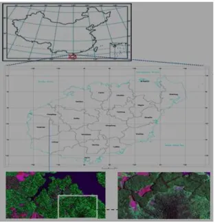
[image:2.595.142.456.157.482.2]Guangba Farm, Dongfang City, was selected as the study area. It is located to the southwest of Hainan Island, China (figure 1). Rubber trees are the major vegetation type in the area; grasses, shrubs, bare area, and surface water also characterize the land-cover type of the study area. A typical area was selected as shown in Scene B of figure 1.
Figure 1. The experimental area.
Data
1)High-resolution remote sensing images
The high-resolution remote sensing images of QuickBird, taken on July 6, 2012, were used in this experiment, a total of 5 spectral images were included; the spatial resolution of the panchromatic image is 0.6 m and that of the multi-spectral regions (red, green, blue, and near-infrared) is 2.4 m. 2)Digital Elevation Model (DEM)
The Advanced Space-borne Thermal Emission and Reflection Radiometer Global Digital Elevation Model (ASTER GDEM), which has a resolution of 30 m, was used in our experiment. 3)Ground truth data
Some ground truth data were derived by GPS between May 2 and May 6, 2015, when the derived time was different from the time taken. However, the derived time and the time taken were the same in a different year, and the vegetation had a similar growing status during the same season. Hence, the ground truth data can be used as the reference data for geometry correction and classification accuracy evaluation of the remote sensing images.
Method
Introduction of C5.0 Decision Tree
For a sample set called S, the target variable C has k types, fq(Ci, S) is the sample number of
S ∈ 𝑆𝑖, |S| is the sample number of sample set S. We can define the information entropy of set S as
info(s) = − ∑ ((fq(Ci,S)
|S| ) × log2( fq(Ci,S)
|S| ))
k
i=1 (1) For an attribute variable T, there are n class types of S, the condition entropy of the attribute T can be defined as:
Cinfo(T) = − ∑ni=1((|Ti|
|T|) × info(Ti)) (2) The information gains of T can be expressed as
Gain(T) = info(s) − Cinfo(T) (3) Hence, the ratio of information gains can be expressed as
Gainrto(T) =Gain(T)
info(s) (4) When we use C5.0 decision tree algorithm, the maximum of Gainrto(T) is the judgment index of the decision features being chosen.
Though the ideal decision tree method is easy, selecting better-fit decision features, especially multiple decision features, is extremely difficult. This is because of two main reasons: 1) we have to scan all features sets when we build a decision tree. This procedure will make the algorithm of C5.0 decision tree inefficient. 2) The C5.0 decision tree method is fit for the data sets that can reside in the memory of computer. when the training sets’ volume is bigger than the computer’s, it is difficult to use them[5],[6] (Galathiya, 2012; Quinlan, 1986). In addition, the value of better-fit decision features is difficult to be evaluated. Obtaining a suitable value of better decision features is another key problem.
Better-Fit Decision Features Selection (BFDFS) Method
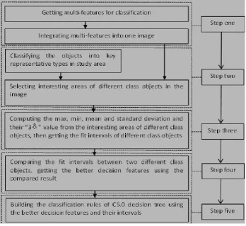
Figure 2. Sketch framework of BFDFS method.
Step one: integrating multi-features into one image file.
All collected features should be integrated together as required for the decision tree method. The process of integrating the multi-features includes standardizing the spatial resolution of all the images, correcting the images according to the same standard, and finally, cutting all the images. Then, all the decision features are stacked into one file, which has the same resolution, coordinate system, and location at last. In our study, we unified all the spectral feature images, vegetation index images, and spatial feature images into the World Geodetic System-1984 coordinate system, interpolated the values in the DEM image according to the spatial resolution of the remote sensing image, corrected the DEM image according to the remote sensing image, cut all the images according to the same area, and stacked all the images into one file using ENVI software.
Step two: selecting interesting areas of every land objects
Users classify the objects into key representative classes based on the users’ experience after integrating multi-features of different images, and select locations of different representative objects for supervised classification (our classification method is a supervised classification method), all are prepared well for the next computing.
Step three: computing values of key representative objects
Users compute the maximum, minimum, mean, and standard deviation of the different representative objects. In addition, users compute the "3σ" value and get the fit intervals of representative objects of each location. The computation theory and process of "3σ" value is as follows.
If X is a normal distribution, which can be expressed as X~N(μ, σ2), X satisfies the rule expressed in equation (15).
P{μ − 3σ ≤ X ≤ μ + 3σ} = 0.9974 (5)
First, we need to compute the “3σ” (3 multiply σ) value of every representative object, and then compare the minimum value with the μ − 3σ value of the representative objects of each location to get their maximum value. The maximum value was used as the lower limit of the value of the representative objects. We also compared the maximum value with the μ + 3σ value of the representative objects of the area of interest to obtain the minimum value, which is used as the upper limit of the value of the representative objects. Hence, the value of every representative object of a location is between its lower and upper limit values. This is also the better-fit intervals of the representative objects of the area of interest.
Step four: Comparing the intervals between two different objects and getting the better-fit decision features according to the reality condition.
[image:5.595.118.491.264.434.2]All the procedures of the decision tree method help the users distinguish between two objects. Distinguishing two objects is a key and difficult job in all procedures. Hence, distinguishing two land objects is prominently described as follows.
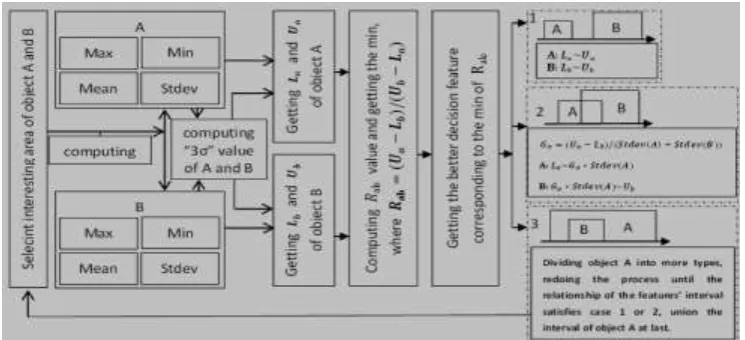
Figure 3. Detailed frameworks of BFDFS method used for distinguishing between object A and B.
We suppose two land objects named A and B, as described in figure 3, are representative objects in an area of interest, Max is the maximum of the object statistical data, Min is the minimum of the object statistical data, Mean is the mean value of the object statistical data (it is also expressed by μ), Stdev is the standard deviation of the object statistical data (it is also expressed by σ), Ua is the upper limit of object A, Ub is the upper limit of object B. We supposed Ua ≥ Ub during the procedure. If Ua≤ Ub, we adjusted the order of object A and B in the same procedure.
The distinguishing procedures between the land objects A and B are as follows:
We selected the area of interest, A and B, which is based on the experiences of users. Hence, users should pay more attention to this procedure, which directly affects the accuracy of the final result. The area around A and B contains all typical features, and all these typical features are prepared well for the decision tree features.
We computed the Max, Min, Mean, and Stdev of every feature of A and B. Then, we systematically computed the “ 3σ” values of the corresponding objects. After comparing the μ − 3σ
We derived equation Rab = (Ua− Lb)/(Ub− La), computed the Rab value of all the features of A and B, where the features of A and B are the same. For example, the procedure of obtaining Rab
of the green spectrum between objects A and B is as follows: We determined the La, Ua, Lb, and
Ub values of the green spectrum of A and B, Rab(green) = (Ua(green) − Lb(green))/
(Ub(green) − La(green)), where Rab(green) is the Rab value of the green spectrum,
Ua(green) is the Ua value of the green spectrum, Lb(green) is the Lb value of the green spectrum, Ub(green) is the Ub value of the green spectrum, and La(green) is the La value of the green spectrum.
After determining the Rab and Rba values of all the features, we sorted the Rab and Rba
[image:6.595.120.484.271.323.2]values in ascending order, selected the front of Rab and Rba (which is also smaller than other feature values) as an option (the count of selected Rab and Rba should be defined according the users’ reality needs). The features corresponding to the selected Rab and Rba are the better-fit decision features of the C5.0 decision tree algorithm if the features’ intervals satisfy case 1 or 2. Here, cases 1, 2, and 3 have been described as follows.
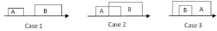
Figure 4. Three distribution cases of interval between object A and B.
The relationship of the interval value of A and B can be grouped into three types, and their distributions are described in figure 4. The first is case 1, in which the intervals of A and B have a separation relationship. In case 2, the intervals of A and B have an intersection relationship. In case 3, the intervals of A and B have an inclusive relationship.
We can get the corresponding features of Rab, and the relationship of the features’ interval value will satisfy one of the cases noted in figure 4. When the relationship agrees with case 1, the feature is the better-fit decision feature of the decision tree, and the decision feature’s value of A is between
La and Ua, and the decision feature’s value of B is between Lb and Ub. When the relationship satisfies case 2, the feature is also the better-fit decision feature of the decision tree, and the decision feature’s value of object A is between La and Gσ∗ Stdev(A), and the decision feature’s value of object B is between Gσ∗ Stdev(A) and Ub, where Gσ = (Ua− Lb)/(Stdev(A) + Stdev(B)). When the relationship satisfies case 3, the feature cannot be the better fit decision feature of the decision tree. In this condition, object A should be divided into two types of new representative objects (new objects A and B). Then, we redid the entire procedure described above until the relationship of the features interval value satisfies case 1 or 2. After distinguishing the two objects, we unified the interval value of the new objects A and B.
Step five: users use the better-fit decision features to build the decision rules for the C5.0 decision tree.
After obtaining the better decision features and their intervals, we can build the decision tree of rubber woods classification based on C5.0 decision tree method.
Experiment and Results
In this experiment, we fuse the red, NIR and green of the remote sensing image, and the DEM data that spatial resolution is 30 m. After being transformed, all the images reserve the land information well while the resolution attains 0.6 m, and all data are in the same coordinate system (GS-1984) in the end. Then we cut the image to satisfy the experimental area, and select NAVI, SAVI (the L value is 0.5), RVI, red, NIR, green, blue to obtain the texture feature data. When all the data (spectral feature, texture feature, and DEM) were collected, we integrated all the data by stacking all the feature data into one file.
(water and bare land are easy to distinguish from rubber woods using spectrum and vegetation index features).
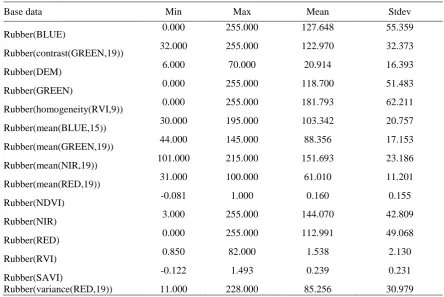
After selecting interesting areas of every key representative land objects, we compute the Min, Max, Mean and Stdev of every key representative land objects(are displayed in table 1), and use the
[image:7.595.74.519.162.459.2]"3σ" theory to obtain the results of fit values of rubber woods, which are displayed in table 2.
Table 1. Statistics of partly fit spectral and spatial features of rubber woods.
Base data Min Max Mean Stdev
Rubber(BLUE) 0.000 255.000 127.648 55.359
Rubber(contrast(GREEN,19)) 32.000 255.000 122.970 32.373
Rubber(DEM) 6.000 70.000 20.914 16.393
Rubber(GREEN) 0.000 255.000 118.700 51.483
Rubber(homogeneity(RVI,9)) 0.000 255.000 181.793 62.211
Rubber(mean(BLUE,15)) 30.000 195.000 103.342 20.757
Rubber(mean(GREEN,19)) 44.000 145.000 88.356 17.153
Rubber(mean(NIR,19)) 101.000 215.000 151.693 23.186
Rubber(mean(RED,19)) 31.000 100.000 61.010 11.201
Rubber(NDVI) -0.081 1.000 0.160 0.155
Rubber(NIR) 3.000 255.000 144.070 42.809
Rubber(RED) 0.000 255.000 112.991 49.068
Rubber(RVI) 0.850 82.000 1.538 2.130
Rubber(SAVI) -0.122 1.493 0.239 0.231
[image:7.595.90.507.482.679.2]Rubber(variance(RED,19)) 11.000 228.000 85.256 30.979
Table 2. Values of partly fit spectral features and spatial features of rubber woods.
Base data 𝟑𝛅 Low
Bound
𝟑𝛅 Upper
Bound Fit low bound
Fit upper bound
Rubber(BLUE) -38.429 293.725 0.000 255.000
Rubber(contrast(GREEN,19)) 25.851 220.088 32.000 220.088
Rubber(DEM) -28.265 70.093 6.000 70.000
Rubber(GREEN) -35.749 273.149 0.000 255.000
Rubber(homogeneity(RVI,9)) -4.840 368.426 0.000 255.000
Rubber(mean(BLUE,15)) 41.072 165.612 41.072 165.612
Rubber(mean(GREEN,19)) 36.897 139.816 44.000 139.816
Rubber(mean(NIR,19)) 82.135 221.251 101.000 215.000
Rubber(mean(RED,19)) 27.407 94.613 31.000 94.613
Rubber(NDVI) -0.305 0.624 -0.081 0.624
Rubber(NIR) 15.643 272.497 15.643 255.000
Rubber(RED) -34.213 260.195 0.000 255.000
Rubber(RVI) -4.852 7.929 0.850 7.929
Rubber(SAVI) -0.454 0.930 -0.122 0.930
Rubber(variance(RED,19)) -7.681 178.192 11.000 178.192
Table 3. Comparison of the partly fit spectral and spatial features of grass and rubber woods.
Grass base data Fit low bound
Fit upper
bound Rubber woods base data
Fit low bound
Fit low
bound R𝑎𝑏 Rba
Grass(BLUE) 0.000 255.000 Rubber(BLUE) 0.000 255.000 1 1
Grass(contrast(GREEN,19)) 0.000 255.000 Rubber(contrast(GREEN,19)) 32.000 220.088 0.87451 0.86309
Grass(DEM) 0.000 255.000 Rubber(DEM) 6.000 70.000 0.976471 0.27451
[image:7.595.54.542.702.789.2]Grass(mean(BLUE,15)) 0.000 255.000 Rubber(mean(BLUE,15)) 41.072 165.612 0.838933 0.649459 Grass(mean(GREEN,19)) -0.900 1.221 Rubber(mean(GREEN,19)) 44.000 139.816 -0.30401 1 Grass(mean(NIR,19)) 0.000 8.230 Rubber(mean(NIR,19)) 101.000 215.000 -0.43149 1 Grass(mean(RED,19)) -0.613 0.830 Rubber(mean(RED,19)) 31.000 94.613 -0.29683 1
Grass(NDVI) 3.495 157.000 Rubber(NDVI) -0.081 0.624 1 -0.01828
Grass(NIR) 6.000 255.000 Rubber(NIR) 15.643 255.000 0.961273 1
Grass(RED) 0.000 237.000 Rubber(RED) 0.000 255.000 0.929412 1
Grass(RVI) 1.895 226.500 Rubber(RVI) 0.850 7.929 1 0.026741
Grass(SAVI) 0.000 255.000 Rubber(SAVI) -0.122 0.930 1 0.003645
[image:8.595.61.535.222.422.2]Grass(variance(RED,19)) 8.897 255.000 Rubber(variance(RED,19)) 11.000 178.192 0.991455 0.687903
Table 4. Comparison of the partly fit spectral and spatial features of shrubs and rubber woods.
Shrub base data Fit low
bound
Fit upper
bound Rubber woods base data
Fit low bound
Fit low
bound R𝑎𝑏 Rba
Shrub(BLUE) 65.437 255.000 Rubber(BLUE) 0.000 255.000 1 0.743384
Shrub(contrast(GREEN,19)) 80.731 255.000 Rubber(contrast(GREEN,19)) 32.000 220.088 1 0.624919
Shrub(DEM) 86.293 255.000 Rubber(DEM) 6.000 70.000 1 -0.06543
Shrub(GREEN) 0.000 76.000 Rubber(GREEN) 0.000 255.000 0.298039 1
Shrub(homogeneity(RVI,9)) 55.179 255.000 Rubber(homogeneity(RVI,9)) 0.000 255.000 1 0.783612 Shrub(mean(BLUE,15)) 0.000 117.195 Rubber(mean(BLUE,15)) 41.072 165.612 0.459647 1 Shrub(mean(GREEN,19)) -0.396 0.572 Rubber(mean(GREEN,19)) 44.000 139.816 -0.30973 1 Shrub(mean(NIR,19)) 0.556 3.397 Rubber(mean(NIR,19)) 101.000 215.000 -0.45514 1 Shrub(mean(RED,19)) -0.264 0.382 Rubber(mean(RED,19)) 31.000 94.613 -0.30271 1
Shrub(NDVI) 98.307 248.000 Rubber(NDVI) -0.081 0.624 1 -0.39375
Shrub(NIR) 133.943 255.000 Rubber(NIR) 15.643 255.000 1 0.505759
Shrub(RED) 166.266 255.000 Rubber(RED) 0.000 255.000 1 0.347976
Shrub(RVI) 146.237 255.000 Rubber(RVI) 0.850 7.929 1 -0.5442
Shrub(SAVI) 193.790 255.000 Rubber(SAVI) -0.122 0.930 1 -0.75595
Shrub(variance(RED,19)) 0.000 129.219 Rubber(variance(RED,19)) 11.000 178.192 0.663436 1
According the BFDFS results, the experimental status satisfies case 3. Therefore, we divided the shrub and grass land objects into shrub land object and grass land object, and reselected the area of interest. Then, we computed and obtained the results of the fit values of the shrub land object and grass land object as in tables 3 and 4.
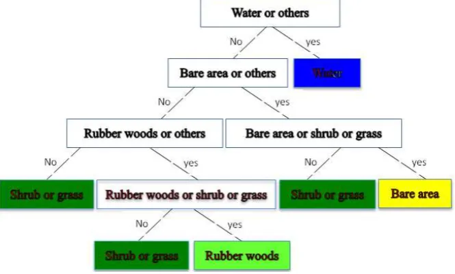
[image:8.595.133.466.533.733.2]After building the decision tree (figure 5), we can choose the better-fit decision features and their value using the BFDFS method, and the decision tree rules of the land object classification are described in table 5.
Figure 5. Classifying decision tree model of rubber woods.
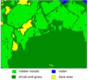
woods’ texture computation window size (here, 19 pixels). The post-processed image is displayed in figure 6.
Figure 6. Classified result image of rubber woods.
Ground truth ROIs (regions of interest) are generated randomly from the QuickBird high-resolution remote sensing images by visual interpretation and GCPs. By comparing the classification results with the ground truth ROIs and GCPs, the error matrix of rubber woods classification is prepared as displayed in table 6. From table 6, we can see that the total accuracy is 92.00%, the Kappa efficient is 0.89, the user accuracy of rubber woods is 91.67%, and the producer accuracy of rubber woods is 88.00%.
Table 6. Rubber woods classification accuracy evaluation.
Reference image
Evaluated image
Rubber woods
Shrub and
grass Bare area water
Total samples
Producer accuracy/ %
Rubber woods 88 12 0 0 100 88.00
Shrub and
grass 8 87 5 0 100 87.00
Bare area 0 6 94 0 100 94.00
Water 0 0 1 99 100 99.00
Total samples 96 105 100 99 400 --
User
accuracy/% 91.67 82.86 94.00 100 -- --
Total accuracy: (368/400)×100%=92.00% kappa=0.89
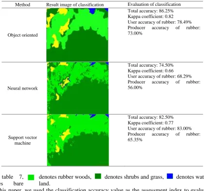
[image:9.595.94.505.511.665.2]Table 7 Classified results and accuracy evaluation of the other method.
Method Result image of classification Evaluation of classification
Object oriented
Total accuracy: 86.25% Kappa coefficient: 0.82
User accuracy of rubber: 78.49% Producer accuracy of rubber: 73.00%
Neural network
Total accuracy: 74.50% Kappa coefficient: 0.66
User accuracy of rubber: 68.29% Producer accuracy of rubber: 56.00%
Support vector machine
Total accuracy: 82.50% Kappa coefficient: 0.77
User accuracy of rubber: 83.00% Producer accuracy of rubber: 65.35%
denotes rubber woods, denotes shrubs and grass, denotes water, In table 7,
denotes bare land.
In this paper, we used the classification accuracy value as the assessment index to evaluate the feasibility of the BFDFS method. According to the theory of the C5.0 decision tree method (described in 3.1 section), the maximum of Gainrto(T) is used to assess the efficiency of the BFDFS method. When the data set is discrete, Gainrto(T) is easy to be computed. However, when the data set is continuous, it is difficult to compute. In our experiment, the values are continuous. Hence, using the maximum Gainrto(T) to evaluate the efficiency of the BFDFS method is not advisable. The classification accuracy of the BFDFS method is proportional to the value of Gainrto(T), which implies a higher accuracy and a bigger value of Gainrto(T). Thus, using the classification accuracy value to evaluate the efficiency of the BFDFS method will be helpful. In addition, the running time of classification in our experiment is less than one minute, which also proves that the BFDFS method is efficient.
Conclusions
The proposed BFDFS is a feasible and efficient method for selecting better-fit decision features. The traditional method of decision features selection is based on the experiences of users, while the BFDFS method is based on computation. Hence, the BFDFS method has a sounder theoretical basis. Furthermore, the classification accuracy of rubber woods proves its feasibility, and the time taken for the classification procedure is less than one minute, which also proves its efficiency.
Acknowledgements
This paper was substantially supported by the Natural Science Foundation of Hainan province, China (Project no. 614225).
References
[1] Kandrika, S., Roy, P. Land use land cover classification of Orissa using multi-temporal IRS-P6 awifs data: A decision tree approach. International Journal of Applied Earth Observation and Geoinformation, 10, 186-193 (2008), http://dx.doi.org/10.1016/j.jag.2007.10.003
[2] Yang, C., Prasher, S., Enright, P., Madramootoo, C., Burgress, M. Application of decision tree technology for image classification using remote sensing data. Agricultural Systems, 76, 1101-1117 (2003).
[3] Punia, M., Joshi, P., Porwal, M. Decision tree classification of land use land cover for Delhi, India using IRS-P6 AWIFS data. Expert Systems with Applications, 38,5577-5583 (2011), http://dx.doi.org/10.1016/j.eswa.2010.10.078
[4] Sesnie, S., Gessler, P., Finegan, B., Thessler, S. Integrating Landsat TM and SRTM-DEM derived variables with decision trees for habitat classification and change detection in complex neotropical environments. Remote Sensing of Environment, 112,2145-2159 (2008), http://dx.doi.org/10.1016/j.rse.2007.08.025
[5] Galathiya, A., Ganatra, A., Bhensdadia, C. Improved decision tree induction algorithm with feature selection, cross validation, model complexity and reduced error pruning. International Journal of Computer Science and Information Technologies, 3(2), 3427-3431 (2012).
[6] Quinlan, J. Induction of decision trees. Machine learning, 1, 81-106 (1986).