R E S E A R C H
Open Access
A new extragradient algorithm for split
equilibrium problems and fixed point
problems
Narin Petrot
1,2, Mohsen Rabbani
3, Manatchanok Khonchaliew
1and Vahid Dadashi
3**Correspondence:
3Department of Mathematics, Sari
Branch, Islamic Azad University, Sari, Iran
Full list of author information is available at the end of the article
Abstract
In this paper, we present a new extragradient algorithm for approximating a solution of the split equilibrium problems and split fixed point problems. The strong
convergence theorems are proved in the framework of Hilbert spaces under some mild conditions. We apply the obtained main result for the problem of finding a solution of split variational inequality problems and split fixed point problems and a numerical example and computational results are also provided.
MSC: 68W10; 65K10; 65K15; 47H09
Keywords: Split equilibrium problem; Pseudomonotonicity; Extragradient method
1 Introduction
LetCandDbe nonempty closed and convex subsets of real Hilbert spacesH1andH2, respectively, and letH1 andH2 be endowed with an inner product ·,· and the corre-sponding norm · . By→and, we denote strong convergence and weak convergence, respectively. Suppose thatf:C×C→Rbe a bifunction. The equilibrium problem (EP) is to findz∈Csuch that
f(z,x)≥0, ∀x∈C. (1.1)
The solution set of the equilibrium problem is denoted byEP(f). The equilibrium prob-lem is a generalization of many mathematical models such as variational inequalities, fixed point problems, and optimization problems; see [6,14,17,18,20,35]. In 2013, Anh [2] in-troduced an extragradient algorithm for finding a common element of fixed point set of a nonexpansive mapping and solution set of an equilibrium problem on pseudomonotone and Lipschitz-type continuous bifunction in real Hilbert space. The author proved the strong convergence of the generated sequence under some condition on it. Since then, many authors considered the EP and related problems and proved weak and strong con-vergence. See, for example [1–4,11,21,26,41].
Moudafi [32] (see also He [25]) introduced the split equilibrium problem (SEP) which is to findz∈Csuch that
z∈EP(f)∩L–1EP(g), (1.2)
whereL: H1→H2is a bounded linear operator andg:D×D→Rbe another bifunction. It is well known that SEP is a generalization of equilibrium problem by consideringg= 0 andD=H2.
He [25] used the proximal method and introduced an iterative method and showed that the generated sequence converges weakly to a solution of SEP under suitable conditions on parameters provided thatf,gare monotone bifunctions onCandD, respectively.
Problem SEP is an extension of many mathematical models which have been considered and studied intensively by several authors recently: split variational inequality problems [12], split common fixed point problems [7,13,16,19,28,31,36,38–40], and the split fea-sibility problems which have been used for studying medical image reconstruction, sensor networks, intensity modulated radiation therapy, and data compression; see [5,8–10] and the references quoted therein.
In this paper, motivated and inspired by the above literature, we consider a new extra-gradient algorithm for finding a common solution of split equilibrium problem of pseu-domonotone and Lipschitz-type continuous bifunctions and split fixed point problem of nonexpansive mappings in real Hilbert space. That is, we are interested in considering the following problem: letH1andH2be real Hilbert spaces andCandDbe nonempty closed and convex subsets ofH1andH2, respectively. Letf:C×C→Randg:D×D→Rbe pseudomonotone and Lipschitz-type continuous bifunctions,T: C→CandS:D→D
be nonexpansive mappings andL: H1→H2 be a bounded linear operator, we consider the problem of finding a solutionp∈Csuch that
p∈EP(f)∩F(T)∩L–1EP(g)∩F(S)=:Ω, (1.3)
whereF(T) is the fixed points set ofTandΩ=∅. Under some mild conditions, the strong convergence theorem will be provided.
The paper is organized as follows. Section2gathers some definitions and lemmas of geometry of real Hilbert spaces and monotone bifunctions, which will be needed in the remaining sections. In Sect.3, we prepare a new extragradient algorithm and prove the strong convergence theorem. In Sect.4, the results of Sect.3are applied to solve split variational inequality problems and split fixed point problem of nonexpansive mappings. Finally, in Sect.5, the numerical experiments are showed and discussed.
2 Preliminaries
We now provide some basic concepts, definitions and lemmas which will be used in the sequel. LetCbe a closed and convex subset of a real Hilbert spaceH. The operatorPCis called a metric projection operator if it assigns to eachx∈Hits nearest pointy∈Csuch that
x–y=minx–z:z∈C.
Lemma 2.1 Let H is a real Hilbert space and C is a nonempty,closed and convex subset of H.Then,for all x∈H,the element z=PCx if and only if
x–z,z–y ≥0, ∀y∈C.
The metric projection satisfies in the following inequality:
PCx–PCy2≤ PCx–PCy,x–y, ∀x,y∈H, (2.1)
therefore the metric projection is firmly nonexpansive operator inH. For more informa-tion concerning the metric projecinforma-tion, please see Sect. 3 of [24].
Lemma 2.2([23]) Let H be a real Hilbert space and T:H→H be a nonexpansive map-ping with F(T)=∅.Then the mapping I–T is demiclosed at zero,that is,if{xn}is a sequence in H such that xnx andxn–Txn →0,then x∈F(T).
Lemma 2.3([42]) Assume that{an}is a sequence of nonnegative numbers such that
an+1≤(1 –γn)an+γnδn, ∀n∈N,
where{γn}is a sequence in(0, 1)and{δn}is a sequence inRsuch that
(i) limn→∞γn= 0, ∞
n=1γn=∞, (ii) lim supn→∞δn≤0.
Thenlimn→∞an= 0.
Lemma 2.4([30]) Let{an}be a sequence of real numbers such that there exists a sub-sequence{ni}of{n}such that ani<ani+1 for all i∈N.Then there exists a nondecreasing sequence{mk} ⊂Nsuch that mk→ ∞as k→ ∞and the following properties are satisfied
by all(sufficiently large)numbers k∈N:
amk ≤amk+1 and ak≤amk+1.
In fact,mk=max{j≤k:aj<aj+1}.
Definition 2.5 A bifunctionf:C×C→Ris said to be • monotone onCif
f(x,y) +f(y,x)≤0, ∀x,y∈C;
• pseudomonotone onCif
f(x,y)≥0 ⇒ f(y,x)≤0, ∀x,y∈C;
• Lipschitz-type continuous onCif there exist two positive constantsc1andc2such that
LetCbe a nonempty closed and convex subset of a real Hilbert spaceHandf :C×C→
Rbe a bifunction, we will assume the following conditions: (A1) f is pseudomonotone onCandf(x,x) = 0for allx∈C;
(A2) f is weakly continuous onC×Cin the sense that ifx,y∈Cand{xn},{yn} ⊂C
converge weakly toxandy, respectively, thenf(xn,yn)→f(x,y)asn→ ∞; (A3) f(x,·)is convex and subdifferentiable onCfor every fixedx∈C;
(A4) f is Lipschitz-type continuous onCwith two positive constantsc1andc2.
It is easy to show that under assumptions (A1)–(A3), the solution setEP(f) is closed and convex (see, for instance [34]).
We need the following lemma to prove our main results.
Lemma 2.6([2]) Assume that f satisfies(A1), (A3), (A4)such thatEP(f)is nonempty and
0 <ρ0<min{21c1,21c2}.If x0∈C,and y0,z0are defined by ⎧
⎨ ⎩
y0=arg min{ρ0f(x0,y) +12y–x02:y∈C},
z0=arg min{ρ0f(y0,y) +12y–x02:y∈C},
then
(i) ρ0[f(x0,y) –f(x0,y0)]≥ y0–x0,y0–y,∀y∈C;
(ii) z0–p2≤ x0–p2– (1 – 2ρ0c1)x0–y02– (1 – 2ρ0c2)y0–z02,∀p∈EP(f).
3 Main results
In this section, we present our main algorithm and show the strong convergence theo-rem for finding a common solution of split equilibrium problem of pseudomonotone and Lipschitz-type continuous bifunctions and split fixed point problem of nonexpansive map-pings in real Hilbert space.
LetH1andH2be two real Hilbert spaces andCandDbe nonempty closed and convex subsets of H1 andH2, respectively. Suppose thatf: C×C→Randg: D×D→Rbe bifunctions. LetL: H1→H2be a bounded linear operator with its adjointL∗,T: C→C andS:D→Dbe nonexpansive mappings andh:C→Cbe aρ-contraction mapping. We introduce the following extragradient algorithm for solving the split equilibrium problem and fixed point problem.
Algorithm 3.1 Choosex1∈H1. The control parametersλn,μn,αn,βn,δnsatisfy the fol-lowing conditions:
0 <λ≤λn≤λ<min
1 2c1
, 1 2c2
, 0 <μ≤μn≤μ<min
1 2d1
, 1 2d2
,
βn∈(0, 1), 0 <lim inf
n→∞ βn≤lim supn→∞ βn< 1, 0 <δ≤δn≤δ< 1 L2,
αn∈
0, 1 2 –ρ
, lim
n→∞αn= 0, ∞
n=1
Let{xn}be a sequence generated by
⎧ ⎪ ⎪ ⎪ ⎪ ⎪ ⎪ ⎪ ⎪ ⎪ ⎪ ⎪ ⎨ ⎪ ⎪ ⎪ ⎪ ⎪ ⎪ ⎪ ⎪ ⎪ ⎪ ⎪ ⎩
un=arg min{μng(PD(Lxn),u) +21u–PD(Lxn)2:u∈D},
vn=arg min{μng(un,u) +12u–PD(Lxn)2:u∈D},
yn=PC(xn+δnL∗(Svn–Lxn)),
tn=arg min{λnf(yn,y) +12y–yn2:y∈C},
zn=arg min{λnf(tn,y) +12y–yn2:y∈C},
xn+1=αnh(xn) + (1 –αn)(βnxn+ (1 –βn)Tzn).
Theorem 3.2 Let H1and H2be two real Hilbert spaces and C and D be nonempty closed
and convex subsets of H1and H2,respectively.Suppose that f: C×C→Rand g: D×D→ Rbe bifunctions which satisfy(A1)–(A4)with some positive constants{c1,c2}and{d1,d2},
respectively.Let L:H1→H2be a bounded linear operator with its adjoint L∗,T:C→C
and S: D→D be nonexpansive mappings,h: C→C be aρ-contraction mapping and
Ω=∅.Then the sequence{xn}generated by Algorithm3.1converges strongly to q=PΩh(q).
Proof Letp∈Ω. So,p∈EP(f)∩F(T)⊂CandLp∈EP(g)∩F(S)⊂D. SincePDis firmly nonexpansive, we get
PD(Lxn) –Lp 2
=PD(Lxn) –PD(Lp) 2
≤PD(Lxn) –PD(Lp),Lxn–Lp
=PD(Lxn) –Lp,Lxn–Lp
= 1
2PD(Lxn) –Lp 2
+Lxn–Lp2–PD(Lxn) –Lxn2
,
and hence
PD(Lxn) –Lp 2
≤ Lxn–Lp2–PD(Lxn) –Lxn 2
. (3.1)
SinceSis nonexpansive,Lp∈F(S) and using Lemma2.6and the definition ofunandvn, we have
Svn–Lp2=Svn–S(Lp)2 ≤ vn–Lp2
≤PD(Lxn) –Lp2– (1 – 2μnd1)PD(Lxn) –un2
– (1 – 2μnd2)un–vn2, (3.2)
for eachn∈N. From (3.1), (3.2) and the assumptions, we obtain
Svn–Lp2≤ Lxn–Lp2–PD(Lxn) –Lxn 2
By (3.3), we get
L(xn–p),Svn–Lxn
=Svn–Lp,Svn–Lxn–Svn–Lxn2
= 1 2
Svn–Lp2–Lxn–Lp2–Svn–Lxn2
≤–1
2PD(Lxn) –Lxn 2
–1
2Svn–Lxn 2.
This implies that
2δn
L(xn–p),Svn–Lxn
≤–δnPD(Lxn) –Lxn2
–δnSvn–Lxn2. (3.4)
SincePCis nonexpansive and by (3.4), we obtain
yn–p2 =PC
xn+δnL∗(Svn–Lxn)
–PC(p) 2
≤(xn–p) +δnL∗(Svn–Lxn) 2
=xn–p2+δn2L∗(Svn–Lxn) 2
+ 2δn
xn–p,L∗(Svn–Lxn)
≤ xn–p2+δn2L2Svn–Lxn2–δnPD(Lxn) –Lxn2–δnSvn–Lxn2
=xn–p2–δn
1 –δnL2Svn–Lxn2–δnPD(Lxn) –Lxn2, (3.5)
then we obtain
yn–p ≤ xn–p. (3.6)
By Lemma2.6, the definition oftnandznand the assumptions we have
zn–p ≤ yn–p, (3.7)
for eachn∈N. From (3.6) and (3.7), we get
zn–p ≤ xn–p. (3.8)
Setqn=βnxn+ (1 –βn)Tzn. It follows from (3.8) that
qn–p ≤βnxn–p+ (1 –βn)Tzn–p ≤βnxn–p+ (1 –βn)zn–p
≤ xn–p. (3.9)
By the definition ofxn+1and (3.9), we obtain
xn+1–p ≤αnh(xn) –p+ (1 –αn)qn–p
≤αnρxn–p+αnh(p) –p+ (1 –αn)xn–p
≤1 –αn(1 –ρ)
xn–p+αn(1 –ρ)
h(p) –p
1 –ρ
≤max
xn–p,
h(p) –p
1 –ρ
.. .
≤max
x1–p,
h(p) –p
1 –ρ
.
This implies that the sequence{xn}is bounded. By (3.6) and (3.8), the sequences{yn}and {zn}are bounded too.
By Lemma2.6, (3.6), the definition ofqnand assumptions onβnandδn, we get
qn–p2≤βnxn–p2+ (1 –βn)Tzn–p2 ≤βnxn–p2+ (1 –βn)zn–p2 ≤βnxn–p2+ (1 –βn)
×yn–p2– (1 – 2λnc1)yn–tn2– (1 – 2λnc2)tn–zn2
≤βnxn–p2+ (1 –βn)
×xn–p2– (1 – 2λnc1)yn–tn2– (1 – 2λnc2)tn–zn2
=xn–p2– (1 –βn)
(1 – 2λnc1)yn–tn2+ (1 – 2λnc2)tn–zn2
.
Therefore,
xn+1–p2≤αnh(xn) –p 2
+ (1 –αn)qn–p2
≤αnh(xn) –p 2
+ (1 –αn)
xn–p2– (1 –βn)
(1 – 2λnc1)yn–tn2
+ (1 – 2λnc2)tn–zn2
,
and hence
(1 –βn)
(1 – 2λnc1)yn–tn2+ (1 – 2λnc2)tn–zn2
≤ xn–p2–xn+1–p2+αnM, (3.10)
where
M=suph(xn) –p 2
–xn–p2+ (1 –βn)
(1 – 2λnc1)yn–tn2
+ (1 – 2λnc2)tn–zn2
,n∈N.
By (3.9), we have
xn+1–p2=αn
h(xn) –p
+ (1 –αn)(qn–p) 2
≤(1 –αn)2qn–p2+ 2αn
≤(1 –αn)2xn–p2+ 2αn
h(xn) –h(p),xn+1–p
+ 2αn
h(p) –p,xn+1–p
≤(1 –αn)2xn–p2+ 2αnρxn–pxn+1–p+ 2αn
h(p) –p,xn+1–p
≤(1 –αn)2xn–p2+αnρ
xn–p2+xn+1–p2
+ 2αn
h(p) –p,xn+1–p
=(1 –αn)2+αnρ
xn–p2+αnρxn+1–p2
+ 2αn
h(p) –p,xn+1–p
. (3.11)
So, we get
xn+1–p2≤
1 –2(1 –ρ)αn 1 –αnρ
xn–p2
+2(1 –ρ)αn 1 –αnρ
αnM0 2(1 –ρ)+
1 (1 –ρ)
h(p) –p,xn+1–p
= (1 –γn)xn–p2
+γn
αnM0 2(1 –ρ)+
1 (1 –ρ)
h(p) –p,xn+1–p
, (3.12)
whereM0=sup{xn–p2,n∈N}, putγn=2(1–1–αnρρ)αn for eachn∈N. By the assumptions on αn, we have
lim
n→∞γn= 0, ∞
n=1
γn=∞. (3.13)
SincePΩhis a contraction onC, there existsq∈Ωsuch thatq=PΩh(q). We prove that
the sequence{xn}converges strongly toq=PΩh(q). In order to prove it, let us consider
two cases.
Case1. Suppose that there existsn0∈Nsuch that{xn–q}∞n=n0 is nonincreasing. In
this case, the limit of{xn–q}exists. This together with the assumptions on{αn},{βn}, {λn}and (3.10) implies that
lim
n→∞yn–tn=nlim→∞tn–zn= 0. (3.14) On the other hands, from the definition ofxn+1and (3.8), we get
xn+1–q2≤αnh(xn) –q2+ (1 –αn)βnxn+ (1 –βn)Tzn–q2
=αnh(xn) –q2+ (1 –αn)
×βnxn–q2+ (1 –βn)Tzn–q2–βn(1 –βn)xn–Tzn2
≤αnh(xn) –q 2
+ (1 –αn)
×βnxn–q2+ (1 –βn)xn–q2–βn(1 –βn)xn–Tzn2
=αnh(xn) –q 2
+ (1 –αn)
xn–q2–βn(1 –βn)xn–Tzn2
and hence
βn(1 –βn)(1 –αn)xn–Tzn2≤αnh(xn) –q 2
+xn–q2
–xn+1–q2. (3.15)
Since the limit of{xn–q}exists and by the assumptions on{αn}and{βn}, we obtain
lim
n→∞xn–Tzn= 0. (3.16)
From (3.9) and (3.11), we have
xn+1–q2–xn–q2– 2αn
h(xn) –q,xn+1–q
≤ qn–q2–xn–q2
≤0. (3.17)
Again, since the limit of{xn–q}exists andαn→0, it follows that
lim
n→∞
qn–q2–xn–q2
= 0
and hence
lim
n→∞qn–q=nlim→∞xn–q, and by (3.9), we get
lim
n→∞xn–q=nlim→∞zn–q. (3.18)
We also get from (3.6), (3.7) and (3.18)
lim
n→∞xn–q=nlim→∞yn–q. (3.19)
By (3.5) and (3.19),
lim
n→∞Svn–Lxn=nlim→∞PD(Lxn) –Lxn= 0, (3.20) which implies that
lim
n→∞Svn–PD(Lxn)= 0. (3.21)
It follows from (3.2) that
(1 – 2μnd1)PD(Lxn) –un 2
+ (1 – 2μnd2)un–vn2
≤PD(Lxn) –Lp2–Svn–Lp2
=PD(Lxn) –Lp+Svn–LpPD(Lxn) –Lp–Svn–Lp
So,
lim
n→∞PD(Lxn) –un=nlim→∞un–vn= 0, (3.22) and hence
lim
n→∞PD(Lxn) –vn= 0. (3.23)
From (3.20) and (3.23), we get
lim
n→∞Lxn–vn= 0. (3.24)
It follows fromxn∈C, the definition ofynand (3.20) that
yn–xn=PC
xn+δnL∗(Svn–Lxn)
–PC(xn) ≤xn+δnL∗(Svn–Lxn) –xn
≤δnLSvn–Lxn →0. (3.25)
Because{xn}is bounded, there exists a subsequence{xnk}of{xn}such that{xnk}
con-verges weakly to somex¯, ask→ ∞and
lim sup
n→∞
xn–q,h(q) –q
= lim
k→∞
xnk–q,h(q) –q
=x¯–q,h(q) –q. (3.26)
Consequently{Lxnk}converges weakly toLx¯. By (3.24),{vnk}converges weakly toLx¯. We
show thatx¯∈Ω. We know thatxn∈Candvn∈D, for eachn∈N. SinceCandDare closed and convex sets, soCandDare weakly closed, therefore,x¯∈CandLx¯∈D. From (3.25) and (3.14), we see that{ynk},{tnk}and{znk}converge weakly tox¯. By (3.22) and (3.23), we
also see that{unk}and{PD(Lxnk)}converge weakly toLx¯. Algorithm3.1and assertion (i)
in Lemma2.6imply that
λnk
f(ynk,y) –f(ynk,tnk)
≥ tnk–ynk,tnk–y
≥–tnk–ynktnk–y, ∀y∈C,
and
μnk
gPD(Lxnk),u
–gPD(Lxnk),unk
≥unk–PD(Lxnk),unk–u
≥–unk–PD(Lxnk)unk–u, ∀u∈D.
Hence, it follows that
f(ynk,y) –f(ynk,tnk) +
1
λnk
and
gPD(Lxnk),u
–gPD(Lxnk),unk
+ 1
μnk
unk–PD(Lxnk)unk–u ≥0, ∀u∈D.
Lettingk→ ∞, by the hypothesis on{λn},{μn}, (3.14), (3.22) and the weak continuity of
f andg(condition (A2)), we obtain
f(x¯,y)≥0, ∀y∈C and g(Lx¯,u)≥0, ∀u∈D.
This means thatx¯∈EP(f) andLx¯∈EP(g). It follows from (3.14), (3.16) and (3.25) that zn–Tzn ≤ zn–tn+tn–yn+yn–xn+xn–Tzn →0.
This together with Lemma2.2implies thatx¯∈F(T). On the other hand, from (3.21) and (3.23), we get
vn–Svn ≤vn–PD(Lxn)+PD(Lxn) –Svn→0,
and using again Lemma2.2, we obtainLx¯∈F(S). Then we proved thatx¯∈EP(f)∩F(T) andLx¯∈EP(g)∩F(S), that is,x¯∈Ω. By Lemma2.1,x¯∈Ωand (3.26), we get
lim sup
n→∞
xn–q,h(q) –q
=x¯–q,h(q) –q≤0. (3.27)
Finally, from (3.12), (3.13), (3.27) and Lemma2.3, we find that the sequence{xn}converges strongly toq.
Case2. Suppose that there exists a subsequence{ni}of{n}such that
xni–q<xni+1–q, ∀i∈N.
According to Lemma2.4, there exists a nondecreasing sequence{mk} ⊂Nsuch thatmk→ ∞,
xmk–q ≤ xmk+1–q and xk–q ≤ xmk+1–q, ∀k∈N. (3.28)
From this and (3.10), we get
(1 –βmk)
(1 – 2λmkc1)ymk–tmk
2+ (1 – 2λ
mkc2)tmk–zmk
2
≤αmkM+xmk–q
2–x
mk+1–q
2
≤αmkM.
This together with the assumptions on{αn},{βn}and{λn}implies that
lim
k→∞ymk–tmk= 0, lim
k→∞tmk–zmk= 0 and lim
From (3.15), we have
βmk(1 –βmk)(1 –αmk)xmk–Tzmk
2≤α
mkh(xmk) –q
2
+xmk–q
2–x
mk+1–q
2
≤αmkh(xmk) –q
2 .
By the hypothesis on{αn}and{βn}, we have
lim
k→∞xmk–Tzmk= 0.
By (3.17), we get
–2αmk
h(xmk) –q,xmk+1–q
≤ xmk+1–q
2–x mk–q
2
– 2αmk
h(xmk) –q,xmk+1–q
≤ qmk–q
2–x mk–q
2≤0.
Since the sequence{xn}is bounded andαn→0, we obtain
lim
k→∞qmk–q=klim→∞xmk–q. By the same argument as Case 1, we have
lim sup
k→∞
xmk–q,h(q) –q
≤0.
It follows from (3.12) and (3.28) that
xmk+1–q
2≤(1 –γ
mk)xmk–q
2+γ mk
αmkM0
2(1 –ρ)+ 1 (1 –ρ)
h(q) –q,xmk+1–q
≤(1 –γmk)xmk+1–q
2+γ mk
α mkM0
2(1 –ρ)+ 1 (1 –ρ)
h(q) –q,xmk+1–q
,
and hence
γmkxmk+1–q
2≤γ mk
α mkM0
2(1 –ρ)+ 1 (1 –ρ)
h(q) –q,xmk+1–q
.
Sinceγmk > 0 and using (3.28) we get
xk–q2≤ xmk+1–q
2≤
αmkM0
2(1 –ρ)+ 1 (1 –ρ)
h(q) –q,xmk+1–q
.
Taking the limit in the above inequality ask→ ∞, we conclude thatxkconverges strongly
toq=PΩh(q).
4 Application to variational inequality problems
space,Cbe a nonempty and convex subset ofHandA:C→Cbe a nonlinear operator. The mappingAis said to be
• monotone onCif
Ax–Ay,x–y ≥0, ∀x,y∈C;
• pseudomonotone onCif
Ax,y–x ≥0 ⇒ Ay,x–y ≤0, ∀x,y∈C;
• L-Lipschitz continuous onCif there exists a positive constantLsuch that
Ax–Ay ≤Lx–y, ∀x,y∈C.
The variational inequality problem is to findx∗∈Csuch that
Ax∗,x–x∗≥0, ∀x∈C. (4.1)
For eachx,y∈C, we definef(x,y) =Ax,y–x, then the equilibrium problem (1.1) be-come the variational inequality problem (4.1). We denote the set of solutions of the prob-lem (4.1) byVI(C,A). We assume thatAsatisfies the following conditions:
(B1) Ais pseudomonotone onC;
(B2) Ais weak to strong continuous onCthat is,Axn→Axfor each sequence{xn} ⊂C converging weakly tox;
(B3) AisL1-Lipschitz continuous onCfor some positive constantL1> 0.
LetH1andH2be two real Hilbert spaces andCandDbe nonempty closed and convex subsets ofH1 andH2, respectively. Suppose that A: C→CandB: D→Dare L1 and L2-Lipschitz continuous onCandD, respectively. LetL:H1→H2 be a bounded linear operator with its adjoint L∗,T: C→CandS: D→Dbe nonexpansive mappings and
h:C→Cbe aρ-contraction mapping. We consider the following extragradient algorithm for solving the split variational inequality problems and fixed point problems.
Algorithm 4.1 Choosex1∈H1. The control parametersλn,μn,αn,βn,δnsatisfy the fol-lowing conditions:
0 <λ≤λn≤λ<L1, 0 <μ≤μn≤μ<L2, βn∈(0, 1),
0 <lim inf
n→∞ βn≤lim supn→∞ βn< 1, 0 <δ≤δn≤δ< 1 L2,
αn∈
0, 1 2 –ρ
, lim
n→∞αn= 0, ∞
n=1
Let{xn}be a sequence generated by ⎧
⎪ ⎪ ⎪ ⎪ ⎪ ⎪ ⎪ ⎪ ⎪ ⎪ ⎪ ⎨ ⎪ ⎪ ⎪ ⎪ ⎪ ⎪ ⎪ ⎪ ⎪ ⎪ ⎪ ⎩
un=PD(PD(Lxn) –μnB(PD(Lxn))),
vn=PD(PD(Lxn) –μnB(un))),
yn=PC(xn+δnL∗(Svn–Lxn)),
tn=PC(yn–λnAyn),
zn=PC(yn–λnAtn),
xn+1=αnh(xn) + (1 –αn)(βnxn+ (1 –βn)Tzn).
Theorem 4.2 Let A:C→C and B: D→D be mappings such that assumptions(B1)–
(B3) hold with some positive constants L1 > 0 and L2 > 0, respectively and Ω :={p∈
VI(C,A)∩F(T),Lp∈VI(D,B)∩F(S)} =∅. Then the sequence {xn} generated by Algo-rithm4.1converges strongly to q=PΩh(q).
Proof Since the mappingAis satisfied the assumptions (B1)–(B3), it is easy to check that the bifunctionf(x,y) =Ax,y–xsatisfies conditions (A1)–(A3). Moreover, sinceAis L1 -Lipschitz continuous onC, it follows that
f(x,y) +f(y,z) –f(x,z) =Ax–Ay,y–z
≥–Ax–Ayy–z
≥–L1x–yy–z
≥–L1 2 x–y
2–L1 2y–z
2, ∀x,y,z∈C.
Thenfis Lipschitz-type continuous onCwithc1=c2=L21, and hencef satisfies condition (A4).
It follows from the definitions off andynthat
tn=arg min
λnAyn,y–yn+ 1 2y–yn
2:y∈C
=arg min
1
2y– (yn–λnAyn) 2
:y∈C
=PC(yn–λnAyn),
and similarly, we can getun=PD(PD(Lxn) –μnB(PD(Lxn))),vn=PD(PD(Lxn) –μnB(un)), and zn=PC(yn–λnAtn). Then the extragradient Algorithm 3.1 reduces to the Algo-rithm4.1and we get the conclusion from and Theorem3.2.
5 Numerical experiments
In this section, we give examples and numerical results to support Theorem3.2. In ad-dition, we compare the introduced algorithm with the parallel extragradient algorithm, which was presented in [27].
We consider the bifunctions f andg which are given in the form of Nash–Cournot oligopolistic equilibrium models of electricity markets [15,34],
g(u,v) = (Uu+Vv)T(v–u), ∀u,v∈Rm, (5.2)
whereP,Q∈Rk×k andU,V ∈Rm×mare symmetric positive semidefinite matrices such thatP–QandU–Vare positive semidefinite matrices. The bifunctionsfandgsatisfy con-ditions (A1)–(A4) (see [37]). Indeed,f andgare Lipshitz-type continuous with constants
c1=c2=12P–Qandd1=d2=12U–V, respectively. Notice that, ifb1=max{c1,d1} andb2=max{c2,d2}, then both bifunctionsfandgare Lipshitz-type continuous with con-stantsb1andb2.
The following numerical experiments are written in Matlab R2015b and performed on a Desktop with Intel(R) Core(TM) i3 CPU M 390 @ 2.67 GHz 2.67 GHz and RAM 4.00 GB.
Example5.1 Let the bifunctionsf andgbe given as (5.1) and (5.2), respectively. We will be concerned with the following boxes:C=ki=1[–5, 5],D=mj=1[–20, 20],C=ki=1[–3, 3] andD=mj=1[–10, 10]. The nonexpansive mappingsT:C→CandS:D→Dare given byT=PCandS=PD, respectively. The contraction mappingh:C→Cis ak×kmatrix such thath< 1, while the linear operatorL:Rk→Rmis am×kmatrix.
In this numerical experiment, the matricesP,Q,U, andVare randomly generated in the interval [–5, 5] such that they satisfy above required properties. Besides, the matrices
handLare randomly generated in the interval (0,1
k) and [–2, 2], respectively. We ran-domly generated starting pointx1∈Rkin the interval [–20, 20] with the following control parameters:δn=21L2,αn=n+21 andμn=λn=4max1{b1,b2}. The following three cases of the
control parameterβnare considered: Case 1. βn= 10–10+n+11 .
Case 2. βn= 0.5. Case 3. βn= 0.99 –n1+1.
Note that to obtain the vectorun, in the Algorithm3.1, we need to solve the optimization problem
arg min
μng
PD(Lxn),u
+1
2u–PD(Lxn) 2
:u∈D
,
which is equivalent to the following convex quadratic problem:
arg min
1 2u
TJu+KTu:u∈D
, (5.3)
whereJ= 2μnV+ImandK=μnUPD(Lxn) –μnVPD(Lxn) –PD(Lxn) (see [27]).
On the other hand, in order to obtain the vectorvn, we need to solve the following convex quadratic problem:
arg min
1 2u
TJu+KTu: u∈D
, (5.4)
Table 1 The numerical results for different parameterβnof Example5.1
Size Average times (sec) Average iterations
k m Case 1 Case 2 Case 3 Case 1 Case 2 Case 3
5 10 1.399695 1.957304 6.356185 37 54 171
10 5 2.168317 2.916557 6.551182 56 75 179
20 50 2.834138 3.785376 8.711813 58 80 186
50 20 5.292192 6.570650 10.418191 111 138 220
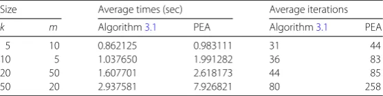
Table 2 The numerical results for the split equilibrium problem of Example5.2
Size Average times (sec) Average iterations
k m Algorithm3.1 PEA Algorithm3.1 PEA
5 10 0.862125 0.983111 31 44
10 5 1.037650 1.991282 36 83
20 50 1.607701 2.618173 44 85
50 20 2.937581 7.926821 80 258
From Table1, we may suggest that a smallest size of parameterβn, asβn= 10–10+n+11 , provides less computational times and iterations than other cases.
Example5.2 We consider the problem (1.3) whenT=IRk andS=IRmare identity
map-pings onRkandRm, respectively. It follows that the problem (1.3) becomes the split equi-librium problem which was considered in [27]. In this case, we compare the Algorithm3.1 with the parallel extragradient algorithm (PEA), which was in [27, Corollary 3.1]. For this numerical experiment, we consider the problem setting and the control parameters as in Example5.1, but only for the case of parameterβnis 10–10+n1+1. The starting pointx1∈Rk is randomly generated in the interval [–5, 5]. We compare Algorithm3.1with PEA by us-ing the stoppus-ing criterionxn+1–xn< 10–3. In Table 2, we randomly take 10 starting points and the presented results are in average.
From Table2, we see that both computational times and iterations of Algorithm3.1are less than those of PEA.
6 Conclusions
We introduce a new extragradient algorithm and its convergence theorem for the split equilibrium problems and split fixed point problems. We also apply the main result to the problem of split variational inequality problems and split fixed point problems. Some nu-merical example and computational results are provided for discussing the possible use-fulness of the results which are presented in this paper. We would like to note that this paper convinces us to consider the future research directions, for example, to consider the convergence analysis and the more general cases of the problem (like the non-convex case) directions; one may see [22,29,33] for more inspiration.
Acknowledgements
The authors are grateful to anonymous referees for their comments and remarks which helped to improve the paper. Vahid Dadashi is supported by Sari Branch, Islamic Azad University.
Funding
This work is partially supported by Naresuan University.
Competing interests
[image:16.595.158.437.202.272.2]Authors’ contributions
All authors contributed equally to the writing of this paper. All authors read and approved the final manuscript.
Author details
1Department of Mathematics, Faculty of Science, Naresuan University, Phitsanulok, Thailand.2Centre of Excellence in
Nonlinear Analysis and Optimization, Faculty of Science, Naresuan University, Phitsanulok, Thailand.3Department of
Mathematics, Sari Branch, Islamic Azad University, Sari, Iran.
Publisher’s Note
Springer Nature remains neutral with regard to jurisdictional claims in published maps and institutional affiliations.
Received: 5 November 2018 Accepted: 30 April 2019 References
1. Anh, P.N.: Strong convergence theorems for nonexpansive mappings and Ky Fan inequalities. J. Optim. Theory Appl.
154, 303–320 (2012)
2. Anh, P.N.: A hybrid extragradient method extended to fixed point problems and equilibrium problems. Optimization
62, 271–283 (2013)
3. Anh, P.N., An, L.T.H.: The subgradient extragradient method extended to equilibrium problems. Optimization64, 225–248 (2015)
4. Anh, P.N., Le Thi, H.A.: An Armijo-type method for pseudomonotone equilibrium problems and its applications. J. Glob. Optim.57, 803–820 (2013)
5. Bauschke, H.H., Borwein, J.M.: On projection algorithms for solving convex feasibility problems. SIAM Rev.38, 367–426 (1996)
6. Blum, E., Oettli, W.: From optimization and variational inequalities to equilibrium problems. Math. Stud.63, 123–145 (1994)
7. Byrne, C., Censor, Y., Gibali, A., Reich, S.: The split common null point problem. J. Nonlinear Convex Anal.13, 759–775 (2012)
8. Censor, Y., Bortfeld, T., Martin, B., Trofimov, A.: A unified approach for inversion problems in intensitymodulated radiation therapy. Phys. Med. Biol.51, 2353–2365 (2006)
9. Censor, Y., Elfving, T.: A multiprojection algorithm using Bregman projections in a product space. Numer. Algorithms
8, 221–239 (1994)
10. Censor, Y., Elfving, T., Kopf, N., Bortfeld, T.: The multiple-sets split feasibility problem and its applications for inverse problems. Inverse Probl.21, 2071–2084 (2005)
11. Censor, Y., Gibali, A., Reich, S.: The subgradient extragradient method for solving variational inequalities in Hilbert space. J. Optim. Theory Appl.148, 318–335 (2011)
12. Censor, Y., Gibali, A., Reich, S.: Algorithms for the split variational inequality problem. Numer. Algorithms59(2), 301–323 (2012)
13. Censor, Y., Segal, A.: The split common fixed point problem for directed operators. J. Convex Anal.16, 587–600 (2009) 14. Combettes, P.L.: The convex feasibility problem in image recovery. In: Hawkes, P. (ed.) Advances in Imaging and
Electron Physics, pp. 155–270. Academic Press, New York (1996)
15. Contreras, J., Klusch, M., Krawczyk, J.B.: Numerical solution to Nash–Cournot equilibria in coupled constraint electricity markets. IEEE Trans. Power Syst.19, 195–206 (2004)
16. Dadashi, V.: Shrinking projection algorithms for the split common null point problem. Bull. Aust. Math. Soc.96(2), 299–306 (2017)
17. Dadashi, V., Khatibzadeh, H.: On the weak and strong convergence of the proximal point algorithm in reflexive Banach spaces. Optimization66(9), 1487–1494 (2017)
18. Dadashi, V., Postolache, M.: Hybrid proximal point algorithm and applications to equilibrium problems and convex programming. J. Optim. Theory Appl.174, 518–529 (2017)
19. Dadashi, V., Postolache, M.: Forward–backward splitting algorithm for fixed point problems and zeros of the sum of monotone operators. Arab. J. Math. (2019).https://doi.org/10.1007/s40065-018-0236-2
20. Daniele, P., Giannessi, F., Maugeri, A.: Equilibrium Problems and Variational Models. Kluwer Academic, Dordrecht (2003)
21. Dinh, B.V., Kim, D.S.: Projection algorithms for solving nonmonotone equilibrium problems in Hilbert space. J. Comput. Appl. Math.302, 106–117 (2016)
22. Gibali, A., Küfer, K.-H., Süss, P.: Successive linear programming approach for solving the nonlinear split feasibility problem. J. Nonlinear Convex Anal.15, 345–353 (2014)
23. Goebel, K., Kirk, W.A.: Topics in Metric Fixed Point Theory. Cambridge Studies in Advanced Mathematics, vol. 28. Cambridge University Press, Cambridge (1990)
24. Goebel, K., Reich, S.: Uniform Convexity, Hyperbolic Geometry, and Nonexpansive Mappings. Dekker, New York (1984) 25. He, Z.: The split equilibrium problem and its convergence algorithms. J. Inequal. Appl. (2012).
https://doi.org/10.1186/1029-242X-2012-162
26. Hieu, D.V., Muu, L.D., Anh, P.K.: Parallel hybrid extragradient methods for pseudomotone equilibrium problems and nonexpansive mappings. Numer. Algorithms73, 197–217 (2016)
27. Kim, D.S., Dinh, B.V.: Parallel extragradient algorithms for multiple set split equilibrium problems in Hilbert spaces. Numer. Algorithms77, 741–761 (2018)
28. Kraikaew, R., Saejung, S.: On split common fixed point problems. J. Math. Anal. Appl.415, 513–524 (2014) 29. Li, Z., Han, D., Zhang, W.: A self-adaptive projection-type method for nonlinear multiple-sets split feasibility problem.
Inverse Probl. Sci. Eng.21, 155–170 (2012)
31. Moudafi, A.: The split common fixed-point problem for demicontractive mappings. Inverse Probl.26, 055007 (2010) 32. Moudafi, A.: Split monotone variational inclusions. J. Optim. Theory Appl.150, 275–283 (2011)
33. Penfold, S., Zalas, R., Casiraghi, M., Brooke, M., Censor, Y., Schulte, R.: Sparsity constrained split feasibility for dose–volume constraints in inverse planning of intensity-modulated photon or proton therapy. Phys. Med. Biol.62, 3599–3618 (2017)
34. Quoc, T.D., Anh, P.N., Muu, L.D.: Dual extragradient algorithms extended to equilibrium problems. J. Glob. Optim.52, 139–159 (2012)
35. Reich, S., Sabach, S.: Three strong convergence theorems regarding iterative methods for solving equilibrium problems in reflexive Banach spaces. Contemp. Math.568, 225–240 (2012)
36. Suwannaprapa, M., Petrot, N., Suantai, S.: Weak convergence theorems for split feasibility problems on zeros of the sum of monotone operators and fixed point sets in Hilbert spaces. Fixed Point Theory Appl.2017, 6 (2017) 37. Tran, D.Q., Muu, L.D., Nguyen, V.H.: Extragradient algorithms extended to equilibrium problems. Optimization57,
749–776 (2008)
38. Tuyen, T.M.: A strong convergence theorem for the split common null point problem in Banach spaces. Appl. Math. Optim. (2017).https://doi.org/10.1007/s00245-017-9427-z
39. Tuyen, T.M., Ha, N.S.: A strong convergence theorem for solving the split feasibility and fixed point problems in Banach spaces. J. Fixed Point Theory Appl.20, 140 (2018)
40. Tuyen, T.M., Ha, N.S., Thuy, N.T.T.: A shrinking projection method for solving the split common null point problem in Banach spaces. Numer. Algorithms (2018).https://doi.org/10.1007/s11075-018-0572-5
41. Vuong, P.T., Strodiot, J.J., Nguyen, V.H.: Extragradient methods and linear algorithms for solving Ky Fan inequalities and fixed point problems. J. Optim. Theory Appl.155, 605–627 (2012)