ISSN 2042-2695
CEP Discussion Paper No 1161
August 2012
Reserve Accumulation, Growth and Financial Crises
Gianluca Benigno and Luca Fornaro
Abstract
We present a model that reproduces two salient facts characterizing the international monetary system: i) Faster growing countries are associated with lower net capital inflows and ii) Countries that grow faster accumulate more international reserves and receive more net private inflows. We study a two-sector, tradable and non-tradable, small open economy. There is a growth externality in the tradable sector and agents have imperfect access to international financial markets. By accumulating foreign reserves, the government induces a real exchange rate depreciation and a reallocation of production towards the tradable sector that boosts growth. Financial frictions generate imperfect substitutability between private and public debt flows so that private agents do not perfectly offset the government policy. The possibility of using reserves to provide liquidity during crises amplifies the positive impact of reserve accumulation on growth. We use the model to compare the laissez-faire equilibrium and the optimal reserve policy in an economy that is opening to international capital flows. We find that the optimal reserve management entails a fast rate of reserve accumulation, as well as higher growth and larger current account surpluses compared to the economy with no policy intervention. We also find that the welfare gains of reserve policy are large, in the order of 1 percent of permanent consumption equivalent.
JEL Codes: F31, F32, F41, F43
Keywords: foreign reserve accumulation, gross capital flows, growth, financial crises
This paper was produced as part of the Centre’s Globalisation Programme. The Centre for Economic Performance is financed by the Economic and Social Research Council.
Acknowledgements
We would like to thank Pierpaolo Benigno, David Cook, Fabrizio Coricelli and José De Gregorio for useful comments. We also thank seminar participants at the London School of Economics, Universitá a Bocconi, the Paris School of Economics, Universitá Cattolica del Sacro Cuore, the Heriot-Watt University and the National Bank of Serbia and participants at the Conference on Financial Stability at the Hong Kong University and the Aix-Marseille Workshop on Open Macroeconomics. Financial support from the ESRC Grant on the Macroeconomics of Capital Account Liberalization is acknowledged. Luca Fornaro acknowledges financial support from the French Ministère de l'Enseignement Supérieur et de la Recherche, the ESRC, the Royal Economic Society and the Paul Woolley Centre.
Gianluca Benigno is an Associate in the Centre for Economic Performance and a Reader in the Economics Department at the London School of Economics and Political Science. Luca Fornaro is a PhD Research Student in the European Doctoral Programme at the Department of Economics, London School of Economics and Political Science.
Published by
Centre for Economic Performance
London School of Economics and Political Science Houghton Street
London WC2A 2AE
All rights reserved. No part of this publication may be reproduced, stored in a retrieval system or transmitted in any form or by any means without the prior permission in writing of the publisher nor be issued to the public or circulated in any form other than that in which it is published.
Requests for permission to reproduce any article or part of the Working Paper should be sent to the editor at the above address.
1
Introduction
One of the most spectacular recent trends in the international monetary system is the considerable built up of foreign exchange reserves by emerging countries, in particular East Asian economies and China.1 As shown by figure 1a, the average reserves-to-GDP
ratio in developing countries more than doubled between 1980 and 2010, increasing from 9.5 to 23.3 percent. The increase has been particularly marked in East Asia, where the average reserves-to-GDP ratio passed from 15.5 percent in 1980 to 55.3 percent in 2010.2
The large accumulation of foreign reserves is not just interesting in itself, but it also represents a key element for understanding the direction and allocation of international capital flows among developing economies. As noticed by Gourinchas and Jeanne (2011), while the neoclassical growth model would suggest that capital should be directed towards those economies that experience faster productivity growth, in the data we observe that faster growing economies are associated with lower net capital inflows (figure 1b).
Public flows, in the form of international reserves, play a fundamental role in ex-plaining this pattern of the data. Gourinchas and Jeanne (2011) show that fast growing countries are net exporters of capital because of their policy of international reserve accu-mulation (figure 1c). Similarly, Alfaro et al. (2011) find that while private flows move in accordance with the neoclassical model, capital outflows from high-productivity emerging markets are driven by the accumulation of official reserves.
In this work we propose an analytical framework that is able to replicate the pattern of international capital flows observed in the data:
• Fact 1: Faster growing countries are associated with lower net capital inflows.
• Fact 2: Countries that grow faster accumulate more international reserves and receive more net private inflows.
We study a two-sector, tradable and non-tradable, small open economy. There are two key elements. First, firms in the tradable sector absorb foreign knowledge by importing intermediate inputs. This mechanism provides the source of growth in our economy, but its benefits are not internalized by individual firms since knowledge can be used freely by all the firms in the economy. Second, private agents have limited access to international financial markets and the economy is exposed to the risk of sudden stops in capital inflows. The presence of growth externalities and financial frictions can explain the direction of capital flows characterizing developing countries. We show that the government can use reserves to exploit the knowledge spillovers in the tradable sector. In fact, an increase in foreign exchange reserves leads to a real currency depreciation and to a reallocation 1See Ghosh et al. (2012) for a discussion of the accumulation of reserves by developing countries in
the last three decades.
2Developing countries refer to a sample of 66 developing economies. East Asia refers to the unweighted
average of China, Hong Kong, Indonesia, South Korea, Malaysia, Philippines, Singapore and Thailand. All the data are from the World Bank Development Indicators.
0 10 20 30 40 50 60 Reserves (% of GDP) Developing countries East Asia
(a) Reserves in percent of GDP
(b) Average per capita GDP growth and average current account balances between 1980 and 2010
(c) Average per capita GDP growth and average reserve accumulation between 1980 and 2010
Figure 1: Motivating facts. Notes: the sample is composed of 66 developing countries. East Asia refers to the unweighted average of China, Hong Kong, Indonesia, South Korea, Malaysia, Philippines, Singapore and Thailand. Data are from the World Bank Development Indicators.
of production toward the tradable sector. This stimulates the use of imported inputs and hence the absorption of foreign knowledge. As a result, economies in which the government accumulates reserves experience faster growth, higher trade surpluses and an undervalued real exchange rate compared to the laissez-faire equilibrium (fact 1).
This mechanism is effective as long as there is imperfect substitutability between private and public flows.3 Indeed, in the neoclassical growth model the accumulation of
international reserves would be offset by private capital inflows. Instead, in our framework the offsetting effect is not complete because the risk of a sudden stop limits the willingness of private agents to accumulate debt in response to an increase in the stock of reserves by the government. Hence, while the economy as a whole runs a current account surplus and gathers foreign reserves, the private sector accumulates foreign liabilities (fact 2).
We also explore the role of reserves as a crisis management tool. By using reserves to provide liquidity to the private sector during financial crises, the government can mitigate the negative impact of sudden stops in capital inflows on production. This represents another channel trough which reserves can positively affect growth. In fact, in our framework the possibility of using reserves during crises amplifies the positive relationship between reserve accumulation and long-run growth.
We then examine the normative implications of reserve accumulation. We first show that a social planner that is unconstrained in terms of policy tools would choose not to accumulate reserves but to rely on sectoral subsidies. We argue, similarly to what Korinek and Serv´en (2010) suggest, that in practice sectoral subsidies may conflict with WTO rules or other trade agreements. In this case, a policy of reserve accumulation can be used to circumvent these restrictions. We compute within a class of simple rules the optimal reserve policy and we find that, despite being a second-best policy tool, the welfare gains from optimal reserve management can be quite large. As an example, we find that the gains from public intervention in capital flows for a country that is opening itself to international capital markets are in the order of 1 percent of permanent consumption equivalents.
The rest of the paper is structured as follows. We start by discussing our key as-sumptions and the related literature. Then, in section 2 we introduce the framework. Section 3 presents the social planning allocation and discusses the political barriers that may prevent a government from implementing the first best through sectoral subsidies. Section 4 provides intuition about the effect of reserve management. Section 5 presents the results of our policy experiment on financial liberalization and provides estimates of the welfare gains from implementing the optimal reserve policy. Section 6 concludes.
Discussion of key elements. Our theory rests on two key elements: the existence of knowledge spillovers in the tradable sector and the limited and intermittent access to 3Imperfect substitutability is in the tradition of Branson and Henderson (1985) and Kouri (1981),
international credit markets. Here we discuss the empirical evidence that underpins these assumptions.
We study an economy that grows by absorbing foreign knowledge. The existence of international knowledge spillovers is well established in the literature on global growth. The foundations for the theoretical study of cross-country knowledge flows were laid down by Grossman and Helpman (1991), while Klenow and Rodriguez-Clare (2005) stress how a model of the world economy has to feature international knowledge spillovers in order to be consistent with the growth patterns observed in the data.
There is also a sizable literature emphasizing the role of trade in facilitating the transmission of knowledge across borders. The idea is that in order to have access to the international pool of knowledge a country has to import foreign products or to export to foreign markets. We choose to focus on the transmission of knowledge through the imports of intermediate inputs because we feel that this is the channel for which more empirical evidence is available. Our starting point is the empirical analysis of Coe et al. (1997). They find that the imports of capital goods and materials represent a key channel through which discoveries made in developed countries spill over to developing economies. Subsequent research, surveyed by Keller (2004), has confirmed the significant role of imports in the process of international knowledge diffusion. More recently, plant-level evidence on the positive impact of imports of intermediate goods on productivity has emerged. For instance, Amiti and Konings (2007) using Indonesian plant-level data find a positive effect on productivity from a decrease in tariffs on intermediate inputs.
Another line of research has tried to identify a positive effect on productivity from ex-porting. This may happen, for example, if exporting allows firms to become familiar with foreign technologies that increase their productivity, the so called learning-by-exporting effect. Isolating this effect is hard, because the most productive firms tend to self-select themselves into the export sector. Despite this difficulty, some firm-level evidence in support of learning-by-exporting effects has been find by Blalock and Gertler (2004), using Indonesian data, and by Park et al. (2010), who use data from Chinese firms. Im-portantly, our qualitative results would carry through in a model in which firms absorb foreign technology by exporting, rather than by importing intermediate inputs.4
In our model productivity growth through the absorption of foreign knowledge is present only in the tradable sector. We make this stark assumption to simplify the expo-sition, but our qualitative results would remain in a setting in which knowledge spillovers are stronger in the tradable sectors compared to the non-tradable ones. Rodrik (2008) provides some indirect evidence consistent with this assumption. He finds that real ex-4There is a long-standing tradition in the growth literature that emphasizes the role of
learning-by-doing effects. This literature, that dates back to Arrow (1962), sees the accumulation of knowledge as a by product of the production process. Krugman (1987) and Young (1991) are early studies of learning-by-doing effects in open economy models. Our qualitative results would hold in a model in which learning-by-doing is the engine of growth, as long as learning-by-doing effects are stronger in the tradable sector and not fully internalized by firms.
change rate depreciations stimulate growth in developing countries and that this effect is increasing in the size of the tradable sector. In addition, Rodrik (2012) considers cross-country convergence in productivity at the industry level and finds that this is restricted to the manufacturing sectors. This finding is consistent with the idea that international knowledge spillovers are confined to, or at least more intense in, the manufacturing sec-tors. Since manufacturing represents the bulk of the sectors producing tradable goods, Rodrik’s finding lends support to our assumption that knowledge spillovers are more important in the tradable sectors.
Finally, in our model knowledge is a non-excludable good, and hence it can be used freely by any firm in the economy. We still lack a good empirical understanding on the extent to which knowledge can be appropriated by individual firms. However, it seems reasonable to assume that, at least partly, the knowledge accumulated inside a firm can spill over to other firms. For example, this may happen trough imitation or through the hiring of workers that embody the technical knowledge developed in a rival firm. Indeed, the assumption that knowledge is only partially excludable is a feature of the most influential endogenous growth frameworks, such as the models developed by Romer (1986), Romer (1990), Grossman and Helpman (1991) and Aghion and Howitt (1992). It is important to stress that, while we assume that knowledge is a completely non-excludable good, the mechanism that we describe would still hold in a framework in which knowledge is partially excludable.
We now turn to our assumptions about financial markets. We consider an economy that periodically sees its access to international credit markets curtailed. This assumption is meant to capture the sudden stop episodes, that is periods in which capital inflows are severely reduced, experienced by many emerging countries. These episodes are often associated with banking crises and deep recessions. In our model, sudden stops have a negative impact on production because they interfere with firms’ ability to secure trade credit and hence to satisfy their demand for imported inputs. Mendoza (2010) shows that a model with this feature is able to capture the behavior of measured TFP around sudden stop episodes. Moreover, Mendoza and Yue (2011) provide empirical evidence on the fall in the use of imported inputs around crisis episodes culminating in a sovereign default. Our specification of financial frictions also allows us to capture the negative long run impact of crises on growth highlighted by the empirical analysis of Cerra and Saxena (2008).
Related literature. This paper is related to several strands of the literature. Our framework provides a plausible explanation for the negative correlation between produc-tivity growth and capital inflows in developing countries observed by Prasad et al. (2007), Gourinchas and Jeanne (2011) and Alfaro et al. (2011). Gourinchas and Jeanne (2011) and Alfaro et al. (2011) find that the allocation of capital among developing economies is driven by the pattern of reserve accumulation and this motivates our focus on foreign
exchange reserves. The central role of government intervention in shaping capital flows to developing countries relates our paper to the so-called “Bretton Woods 2” perspective on the international monetary system of Dooley et al. (2003), according to which the large accumulation of international reserves by the public sector in emerging economies is part of an export-led growth strategy. Our paper is also related to Rodrik (2008), who pro-vides empirical evidence in favor of a causal link from real exchange rate undervaluation to growth.
From a theoretical perspective, our paper is connected to the growing literature pro-viding formal models that reproduce the negative correlation between growth and capital inflows characterizing developing countries. Examples include Aghion et al. (2006), An-geletos and Panousi (2011), Broner and Ventura (2010) and Sandri (2010). These papers all focus on private capital flows, while in our model the negative correlation between growth and capital inflows is driven by reserve accumulation by the public sector. Aguiar and Amador (2011) provide a model in which public flows may generate a negative cor-relation between growth and capital inflows, but the mechanism that they emphasize is different from ours. In fact, in their model the government decreases its stock of foreign debt in order to credibly restrain from expropriating the return from private investment, thus stimulating investment and growth. In contrast, in our framework reserve accumu-lation by the public sector shifts productive resources toward the tradable sector in order to exploit the knowledge spillovers coming from the imports of foreign capital goods.
Our paper is also related to that fast growing literature that examines the deter-minants of reserve accumulation in emerging markets. Aizenman and Lee (2007) and Korinek and Serv´en (2010) emphasize the link between reserve accumulation and growth externalities, while Durdu et al. (2009) and Jeanne and Ranci`ere (2011) focus on the precautionary motive of holding international reserves. Bacchetta et al. (2011) suggest that the accumulation of foreign reserves can be used to supply saving instruments to domestic agents when domestic financial markets are imperfect and private agents have limited access to foreign credit. Our framework encompasses the first two approaches and differs critically from the existing literature in the modeling of public versus private capital flows.
2
Model
We consider an infinite-horizon small open economy. Time is discrete and indexed by
t. The economy is populated by a continuum of mass 1 of households and by a large number of firms. The firms are owned by the households and produce tradable and non-tradable consumption goods. Firms producing the tradable good engage in financial transactions with foreign investors. There is also a government that manages foreign exchange reserves.
2.1
Households
The representative household derives utility from consumption and supplies inelastically one unit of labor each period. The household’s lifetime expected utility is given by
E0 " ∞ X t=0 βtC 1−γ t 1−γ # . (1)
In this expression, Et[·] is the expectation operator conditional on information available at timet ,β <1 is the subjective discount factor, γ >0 is the coefficient of relative risk aversion and Ct denotes a consumption composite good. Ctis defined as a Cobb-Douglas aggregator of tradable CtT and non-tradableCtN consumption goods5
Ct = CtT
ω
CtN1−ω
, (2)
where 1 > ω > 0 denotes the share of expenditure in consumption that the household allocates to the tradable good.
Each period the household faces the following flow budget constraint
CtT +PtNCtN =Wt+ ΠTt + Π N
t . (3)
The budget constraint is expressed in units of the tradable good. The left-hand side repre-sents the household’s expenditure. We definePN
t as the relative price of the non-tradable good in terms of the tradable good, so CT
t +PtNCtN is the household’s consumption ex-penditure expressed in units of the tradable good. The right-hand side represents the income of the household. Wt denotes the household’s labor income. ΠTt and ΠNt are the dividends that the household receives from firms operating respectively in the tradable and in the non-tradable sector. For simplicity, we have assumed that domestic households do not trade directly with foreign investors. As we will see below, households can access international financial markets indirectly through their ownership of firms.
Each period the representative household chooses CT
t and CtN to maximize expected utility (1) subject to the budget constraint (3). The first order conditions are
ωCt1−γ CT t =λt (4) (1−ω)Ct1−γ CN t =λtPtN, (5)
where λt denotes the Lagrange multiplier on the budget constraint, or the household’s marginal utility of wealth. By combining (4) and (5), we obtain the standard intratem-poral equilibrium condition that links the relative price of non-tradable goods to the 5A Cobb-Douglas consumption aggregator is needed to ensure the existence of a balanced growth
marginal rate of substitution between tradable and non-tradable goods PtN = 1−ω ω CtT CN t . (6)
According to this expression, PN
t is increasing in CtT and decreasing in CtN. In what follows we will use PN
t as a proxy for the real exchange rate.
2.2
Firms in the tradable sector
The tradable sector is meant to capture a modern sector characterized by dynamic pro-ductivity gains and open to financial transactions with foreign investors. Firms in the tradable sector produce using laborLT
t, an imported intermediate inputMtand the stock of accumulated knowledge Xt, according to the production function
YtT = XtLTt
αT
M1−αT
t , (7)
where YT
t is the amount of tradable goods produced in period t and 0< αT < 1 is the labor share in gross output in the tradable sector. Knowledge is non-rival and can be freely used by firms producing tradable goods.
Firms in the tradable sector have access to international credit markets and can trade in a non-contingent one period bond denominated in units of tradable goods that pays a fixed interest rate R. At the end of the period the representative firm distributes to the households the dividends
ΠTt =YtT −WtLTt −P MM
t−Bt+1+RBt−Tt. (8) where Bt denotes the firm’s holding of foreign bonds at the start of period t, Wt is the wage paid to workers in the tradable sector, PM is the price of the imported input and
Tt are lump-sum taxes paid to the government.6
We assume that the tradable sector is subject to a working capital constraint. A fraction φ of the intermediate inputs has to be paid at the beginning of the period and requires working capital financing. To finance their working capital, firms have access to intraperiod loan contracts. Under these contracts, the funds borrowed by firms at the start of the period have to be repaid at the end of the same period. We assume that the interest rate charged on intraperiod loans is equal to zero. The domestic government provides an amount Dt of working capital loans. The remaining part φPMMt−Dt has to be covered using intraperiod loans from foreign investors.
In addition, we introduce financial frictions by assuming that at the end of the period each firm can choose to default on its debts toward international investors. In case of 6The assumption that taxes are paid by firms in the tradable sector, rather than by households, is
default international investors are able to collect an amount of tradable goods equal to
κtXt. To prevent defaults, international investors impose on domestic firms the borrowing constraint
φPMMt−Dt−RBt ≤κtXt, (9)
where κt measures the tightness of the borrowing constraint. On the left-hand side, we have net liabilities of the firms at the beginning of period t. Notice that both the intertemporal loans and the loans used to finance the working capital expenses enter the constraint. We introduce credit shocks in the model by assuming that the parameter
κt is stochastic. In what follows we refer to a financial crisis as a period in which the borrowing constraint (9) holds with equality.
Each period the representative firm choosesLT
t,MtandBt+1to maximize its expected
stream of dividends discounted by the households’ marginal utility of wealth
E0 " ∞ X t=0 βtλtΠTt # , (10)
subject to the borrowing constraint (9). The optimality conditions are given by
αTYtT =WtLTt (11) (1−αT)YtT =P MM t 1 +φµt λt (12) λt=βREt[λt+1+µt+1] (13) µt φPMMt−Dt−RBt−κtXt = 0, µt≥0, (14)
whereµtdenotes the multiplier on the borrowing constraint. Equation (11) represents the optimal demand for labor, which implies equality between the marginal product of labor and the wage. The optimal demand for imported inputs is given by equation (12). When the borrowing constraint is not binding (µt = 0), the marginal product of the imported input is equated to its price. When the borrowing constraint is binding (µt>0), firms are unable to purchase the optimal amount of imported inputs. This shows up in the equation as an increase in the marginal cost of purchasing one unit of the imported input. Equation (13) is the modified Euler equation for the case in which international borrowing might be constrained. The expectation of a future binding borrowing constraint has an effect similar to an increase in the cost of intertemporal debt that induces agents to decrease their borrowing. Finally, equation (14) is the complementary slackness condition for the borrowing constraint.
2.3
Knowledge accumulation
The stock of knowledge available to firms in the tradable sector evolves according to
Xt+1 =ψXt+MtξX 1−ξ
t , (15)
where ψ ≥0 and 0 ≤ξ ≤ 1. This formulation captures the idea that imports of foreign capital goods represent an important transmission channel through which discoveries made in developed economies spill over to developing countries. As mentioned above, we assume that knowledge is a non-rival and non-excludable good. This, combined with the assumption of a large number of firms in the tradable sector, implies that firms do not internalize the impact of their actions on the evolution of the economy’s stock of knowledge.
2.4
Firms in the non-tradable sector
The non-tradable sector represents a traditional sector with stagnant productivity, closed to financial transactions with foreign investors. The non-tradable good is produced using labor, according to the production function YN
t = LNt
αN . YN
t is the output of the non-tradable good, LN
t is the amount of labor employed and 0 < αN < 1 is the labor share in gross output in the non-tradable sector.7
The dividends distributed by firms in the non-tradable sector can be written as
ΠNt =PtNYtN −WtLNt . (16)
In this expression we have used the fact that in equilibrium firms in both sectors produce and that this requires equalization between the wages offered in the two sectors. Profit maximization implies αNPtNL N t αN−1 =W t. (17)
This equation represents the optimal demand for labor from firms in the non-tradable sector. As before, the marginal product of labor is equated to the wage rate.
2.5
Credit shocks
The only source of uncertainty in the model concerns κt, the parameter that governs the sum that foreign lenders can recover in case of default. Our aim is to model an economy in which tranquil times alternate with crises. The simplest way to capture this is to assume that κt can take two values, κH and κL with κH > κL. We will choose values for 7To ensure constant returns to scale in the production of non-tradable goods, we can assume that
production is carried out using labor and land according to a constant-returns-to-scale Cobb-Douglas aggregator. The production function in the main text obtains if the supply of land is fixed and normalized to one.
κH such that when κt =κH the borrowing constraint (9) does not bind, while the value for κL will be such that when κt=κL the borrowing constraint may bind, depending on
Bt and on the actions of the government. As mentioned above, we refer to a period in which the borrowing constraint binds as a financial crisis. Moreover, denoting by ρi for
i=H, L the probability of κt=κi knowing that κt−1 =κi, we will set ρH >0.5 so that crises are rare events and ρL>1−ρH so that crisis events have some persistence.
2.6
Government
The government collects taxes from firms in the tradable sector Tt, provides working capital loans Dt to firms and trades in foreign exchange reserves F Xt. In the spirit of Gertler and Karadi (2011), we assume that lending from the government entails some efficiency losses. Specifically, we assume that in order to lend to firms a sum equal toDt, the government has to employ an amount of tradable goods equal to Dt/(1−θ), with 0 ≤ θ ≤ 1. Of this amount, Dt is repaid by firms to the government at the end of the period, while Dtθ/(1−θ) is lost during the intervention. Hence, the higherθ is, the less efficient is the government in providing liquidity to firms.
We can then write the government budget constraint expressed in units of tradable goods as
F Xt+1 =RF XF Xt+Tt−Dt
θ
1−θ, (18)
whereRF X is the gross interest rate paid on reserves. To capture some salient features of foreign exchange reserves, we assume that the interest rate paid on reserves is not greater than the interest rate charged on private loans (RF X ≤ R) and that the government cannot hold negative amounts of foreign reserves
F Xt ≥0. (19)
Moreover, the resources employed to provide working capital loans to firms at the start of the period cannot exceed the start of period holdings of foreign reserves
Dt
1−θ ≤R
F X
F Xt. (20)
To simplify the analysis, we restrict our attention to simple forms of intervention. In particular, we assume that to finance reserve accumulation the government levies a tax equal to a fractionχof the output of tradable goods during tranquil times, while following a bad credit shock the government sets the tax to zero. More formally, we assume that
Tt= ( χYT t if κt=κH 0 if κt=κL (21)
to firms until their borrowing constraint stops binding or until the size of the intervention exceeds a fractionχW K of the start-of-period stock of reserves. Formally, we assume that
Dt=max φPMMtunc−RBt−κtXt, χW K(1−θ)RF XF Xt
, (22)
where 0 ≤ χW K ≤ 1 and Mtunc is the amount of intermediate inputs that firms would choose in absence of financial frictions, that is ifφ = 0.
2.7
Market clearing and competitive equilibrium
Market clearing for the non-tradable goods requires that the amount consumed is equal to the amount produced
CtN = LNt αN
. (23)
Combining (23), with the households’ budget constraint (3), the definitions of firms’ profits in the tradable and non-tradable sectors (8) and (16), and the government budget constraint (18), we obtain the market clearing condition for the tradable good
CtT =YtT −PMMt−Bt+1+RBt−F Xt+1+RF XF Xt−
θ
1−θDt. (24)
Finally, equating the demand and supply of labor gives
LTt +LNt = 1. (25)
We are now ready to define a rational expectation equilibrium as a set of stochastic processes {Ct, CtT, CtN, PtN, λt, YtT, LTt, LNt , Mt, Bt+1, µt, Wt, Xt+1, F Xt+1, Tt, Dt}∞t=0
satis-fying (2), (4)-(7), (11)-(14), (17)-(18) and (21)-(25), given the exogenous process{κt}
∞
t=0,
the government policy χ, χW K and initial conditions B0, F X0 and X0.
The model has a balanced growth path in which CtT, YtT, Mt, PtN, Bt+1 and Wt all grow at the same rate as Xt. The real exchange rate grows at a positive rate in the balanced growth path because productivity in the tradable sector exhibits positive trend growth, while productivity in the non-tradable sector is fixed. This is the classic Balassa-Samuelson effect. Since also GDPt = YtT −PMMt+PtNYtN grows at the same rate as
Xt, we will refer to the growth rate of the stock of knowledge as the growth rate of the economy.
2.8
Discussion: public and private capital flows
A novel feature of our framework is the distinction between public capital flows in the form of foreign reserves (F Xt) and private capital flows (Bt). Before we move forward in the analysis, we want to emphasize the roots of the imperfect substituability between the internationally traded private bond and foreign reserves.
The first difference is related to the fact that in our framework domestic agents have an imperfect access to international private capital markets. In fact, domestic agents are subject to an occasionally binding borrowing constraint that limits their access to foreign credit. Crucially, the possibility of the constraint being binding in the future affects agents’ behavior also when they are not constrained. In particular, a positive probability of hitting the constraint in the future limits the accumulation of private debt during periods in which access to foreign credit is plentiful. We also assume that foreign reserves provide a lower return compared to private bonds (RF X ≤ R). Moreover, similarly to what is also assumed in a first-generation currency crises model, reserves are subject to a lower bound (F Xt≥0) so that they can only be accumulated.
These features make the two assets imperfect substitutes. We note here that imperfect substitutability between Bt and F Xt would hold even if RF X = R as long as there is a possibility that the borrowing constraint that private agents face might be binding. This feature of the model creates the key difference with respect to the neoclassical growth model in which the accumulation of foreign reserves would be exactly offset one-for-one by private capital inflows. It also differs from the tradition in international finance as in Kouri (1981) and Branson and Henderson (1985) in which imperfect substitutability is exogenously assumed rather than arising endogenously. From our reading of the literature the distinction between the private and public nature of capital flows is novel and differs from existing contributions that identify the international reserves accumulated by the government with the economy’s stock of net foreign assets.
Reassuringly, our model is consistent with the cyclical pattern of gross capital flows characterizing developing countries as described by Broner et al. (2011). In our framework tranquil times are periods of positive capital inflows, in the form of increases in private debt, as well as positive capital outflows, in the form of accumulation of official reserves. Conversely, during crises there is a retrenchment in gross capital flows. Capital inflows diminish as firms cut their stock of foreign debt, while capital outflows fall because the government employs its stock of reserves to mitigate the impact of the crisis. Because of these effects, in our model gross capital outflows are procyclical, consistent with the findings of Broner et al. (2011).8
3
Social planner
Before considering the foreign reserve policy, we first characterize the social planner allo-cation. This is useful to build intuition about the source of inefficiency in the competitive equilibrium that creates scope for policy intervention.
The planner maximizes domestic households’ utility (1), subject to the economy-wide resource constraints (23), (24) and (25), the borrowing constraint (9) and the two 8Moreover, Broner et al. (2011) find that developing countries reduce their stock of official reserves
constraints on reserve management (19) and (20). Importantly, the social planner takes into account the effect that imported inputs have on the accumulation of knowledge, and so also the equation describing the evolution of the stock of knowledge (15) enters as a constraint in the planner’s problem.
Appendix A provides a formal characterization of the social planning allocation. Here we notice that, as long as RF X < R, the social planner chooses not to hold reserves, that is she sets F Xt+1 = 0 for every t.9 Intuitively, the social planner chooses not to hold
reserves because they represent an inefficient saving vehicle compared to foreign bonds, as they pay a lower interest rate. This happens notwithstanding the fact that reserves can be used to provide liquidity during crises. To understand this result, notice that the working capital constraint is affected by the private net foreign asset position at the beginning of periodt. Due to the lower interest rate paid on reserves compared to private bonds, the most efficient way from the social planner perspective to relax the constraint in periodt is by reducing the net debt position in periodt−1 (i.e. increasingBt), rather than accumulating reserves and using them in the event of a crisis.
As showed in appendix A, the social planner allocation is characterized by the same equations as the competitive equilibrium in which F Xt+1 = Dt = 0 is imposed in every period.10 The only difference is given by equation (12), the optimality condition that determines the choice of imported inputs. In fact, in the social planner allocation equation (12) is replaced by PM 1 +φµ SP t λSP t = (1−αT) YT t Mt +βξ Xt Mt 1−ξ Et λSP t+1 λSP t αT YT t+1 Xt+1 +κt+1 µSP t+1 λSP t+1 | {z } growth externality ,
where µSPt is the Lagrange multiplier on the borrowing constraint (9) and λSPt is the Lagrange multiplier on the resource constraint for tradable goods (24). The left-hand side of this expression represents the marginal cost of increasing the use of imported inputs, taking into account the impact of the borrowing constraint, captured by the term
µSPt . The first term on the right-hand side is the benefit from the increase in the output of tradable goods generated by an increase in the use of imported inputs. These two terms are equivalent to the ones that would arise in the competitive equilibrium allocation (12). The second term on the right-hand side is specific to the social planner problem and captures the benefits derived from the increase in the stock of knowledge implied by an increase in the use of imported inputs. Increasing the stock of knowledge is beneficial for two reasons. First, the social planner internalizes the fact that a higher usage of imported
9If RF X = R the planner may hold foreign reserves, but imposing F X
t+1 = 0 for every t on her
allocation does not prevent the planner from reaching the first best. See the appendix for the details.
10To be precise, if the economy starts with a positive amount of reserves (F X
0 >0) and it is hit by
a bad credit shock during the first period (κ0=κL) the planner may use the initial stock of reserves to
finance working capital andD0 may be positive. Even in this case,F Xt+1= 0 for anyt and soDt= 0
inputs today leads to higher knowledge and higher productivity tomorrow and thus to a higher amount of tradable goods produced in the future. Second, the social planner internalizes the fact that an increase in productivity tomorrow relaxes the borrowing constraint by increasing the sum that foreign investors can recover in case of default. These two effects imply that in every period the amount of imported inputs used is higher in the social planner allocation than in the competitive equilibrium without policy intervention. Because of this, the economy grows at a faster rate under the social planner allocation compared to the competitive equilibrium with no policy intervention.
It is possible to decentralize the social planner allocation in the competitive equilib-rium by subsidizing the purchase of imported inputs at rate
τt = βξ PM Xt Mt 1−ξ Et λSP t+1 λSP t αT YT t+1 Xt+1 +κt+1 µSP t+1 λSP t+1 ,
while financing the subsidy using lump-sum taxes. This subsidy scheme is able to re-store the first best, but in practice this form of intervention might be politically hard to implement. For instance, a government might not be able to openly subsidize firms in the export sector due to the existence of trade agreements such as the WTO rules. In the next section we show how an appropriate management of foreign exchange reserves can serve as a second best policy to internalize the growth externalities in the tradable sector, without breaking the rules dictated by free trade agreements.
4
Reserve policy and growth
In this section we discuss the mechanisms through which a policy of reserve accumulation during tranquil times and liquidity provision during crisis times works. In particular we are interested in providing intuition on how foreign reserves can be used as a second best policy tool aimed at internalizing the growth externalities in the tradable sector.
We start by examining the impact of foreign reserve accumulation in states in which the borrowing constraint is not binding. Combining equations (11), (12) and (17) and using the fact that when the borrowing constraint does not bind µt = 0, we obtain the demand for imported inputs,Mt, as a function of the real exchange rate, PtN
Mt= 1−αT PM αT1 Xt 1− αN αT PN t Xt PM 1−αT 1−αT αT 1 1−αN .
When the real exchange rate appreciates (PN
t rises) the demand for imported inputs de-creases. Intuitively, an increase inPN
t , the relative price of non-tradable goods, increases the marginal product of labor in the non-tradable sector. This causes a shift of labor out of the tradable sector that decreases the productivity of the imported intermediate
inputs and induces firms to reduceMt. This suggests that in order to increase the use of imported inputs and the growth rate of the economy above their competitive equilibrium values, the government can implement policies that reducePN
t , that is to engineer a real exchange rate undervaluation.11
To understand the link between reserve accumulation and real exchange rate determi-nation in tranquil times, we combine equations (6), (18) and (24) and use the fact that during tranquil times Dt= 0 to obtain
PtN = 1−ω ω YtT −PMMt−Bt+1+RBt−F Xt+1+RF XF Xt CN t .
Holding everything else constant, this equation implies a negative relationship between
PtN and F Xt+1. The intuition is simple: In order to accumulate foreign reserves the
government needs to withdraw resources from the private sector. Since only tradable goods can be sold to foreigners in exchange for reserves, the government must appropriate tradable goods from the private sector.12 Private agents are then forced to reduce their consumption of tradable goods. This leads to a real exchange rate depreciation which in turns stimulates production in the tradable sector and imports of the intermediate good. Through this channel, a policy of accumulating reserves during tranquil times has the potential to increase the growth rate of the economy and to internalize, at least partly, the growth externalities present in the tradable sector.
Clearly, in general equilibrium a change in F Xt+1 affects all the other endogenous
variables. In particular private agents tend to offset the impact of the increase in foreign reserves on consumption by borrowing from abroad. Indeed, in a model in which private borrowing and reserves are perfect substitutes, the accumulation of F Xt+1 would be
counterbalanced by a corresponding decline in Bt+1. In our framework the imperfect
substitutability between the two assets prevents private agents from completely offsetting the actions of the government.
We now illustrate the general equilibrium implications of a policy of reserve accumu-lation during tranquil times by examining how the stochastic steady state of our economy varies when we change the value ofχ, our proxy for the resources employed to accumulate reserves during tranquil times.13
The six panels of figure 2 show the long-run mean values of the following variables: the growth rate of GDP, the percentage deviations of the real exchange rate from its value in the equilibrium with no policy intervention, the trade balance-to-GDP ratio, the 11We refer to a policy-induced real exchange rate undervaluation when the real exchange rate, net
of the Balassa-Samuelson effect, is undervalued in the competitive equilibrium allocation with policy intervention compared to its value in the laissez-faire equilibrium.
12In our model, we can think of tradable goods as a proxy for the international currency.
13More precisely, for each value ofχwe solved the model numerically. Then we drew a 10000
periods-long simulation, discarded the first 100 periods, and computed the periods-long run average values of the variables of interest. In all the simulations we set χW K = 0, details on the value of the other parameters are provided in section 5.1.
0 0.05 0.1 0.15 0.03 0.035 0.04 0.045 χ GDP growth 0 0.05 0.1 0.15 −0.04 −0.03 −0.02 −0.01 0 χ
Real exchange rate
0 0.05 0.1 0.15 0 0.02 0.04 0.06 0.08 χ Trade balance/GDP 0 0.05 0.1 0.15 −0.17 −0.168 −0.166 −0.164 −0.162 −0.16 χ
Private net foreign assets/GDP
0 0.05 0.1 0.15 0.148 0.15 0.152 0.154 0.156 0.158 0.16 0.162 χ Consumption of tradables 0 0.05 0.1 0.15 0.39 0.395 0.4 0.405 0.41 0.415 χ Aggregate consumption
Figure 2: Impact of reserve accumulation. Notes: χis the fraction of tradable output devoted to reserve accumulation during tranquil times. The real exchange rate, net of the Balassa-Samuelson effect, refers to the percentage change of PtN/Xt with respect to its value in absence of government intervention
(χ= 0). The trade balance is defined asYtT−PMMt−CtT. The private net foreign assets-to-GDP ratio
is defined asBt+1/GDPt. Consumption is normalized by the stock of knowledge. In all the simulations
we setχW K= 0, details on the value of the other parameters are provided in section 5.1.
private net foreign assets-to-GDP ratio, consumption of tradable goods and aggregate consumption as a function of χ, the fraction of tradable output devoted to reserve ac-cumulation during tranquil times. The real exchange rate is normalized by the stock of knowledge to control for the Balassa-Samuelson effect. The same normalization is applied to consumption of tradable goods and to aggregate consumption.
As suggested by the partial equilibrium analysis, the growth rate of the economy is increasing in the amount of resources devoted to reserves accumulation during tranquil times. Stronger accumulation of foreign exchange reserves also produces a depreciation of the real exchange rate and an increase in the trade balance-to-GDP ratio. Both of these effects are driven by the fall in the consumption of tradable goods caused by the withdrawal of resources from private agents. The increase in the production of tradable goods implied by the real exchange rate depreciation also contributes to the improvement in the trade balance-to-GDP ratio.
Figure 2 shows that as the government increases the pace at which it accumulates foreign exchange reserves the private foreign debt-to-GDP ratio rises. As we mentioned above, this occurs as private agents partially offset the increase in public savings implied by faster reserve accumulation by decreasing private savings and hence by accumulating more foreign debt.14
De-trended consumption of tradable goods and aggregate consumption are both de-creasing in the rate of reserve accumulation. This highlights a key trade-off that deter-mines the impact on welfare of government intervention. On the one hand, faster reserve accumulation induces higher growth and this has a positive effect on welfare. On the other hand, in order to accumulate foreign exchange reserves the government has to sub-tract resources that would otherwise be consumed, and this affects welfare negatively. The balance between these two effects determines whether reserve accumulation during tranquil times has a positive or negative impact on welfare, as we will document later.
We now turn to the impact of crisis-times interventions. During crisis times, the borrowing constraint binds and the amount of imported inputs used in production is given by
Mt=
XtκL+RBt+Dt
φPM .
This equation makes clear that in order to increase the amount of imported inputs used by firms above its value in the equilibrium without intervention, the government has to provide working capital loans during crisis events (i.e. set Dt > 0). Hence, in the model the existence of growth externalities in the tradable sector, coupled with financial frictions, provides a justification for the use of reserves during crises.
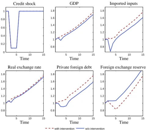
Figure 3 compares the response to a negative credit shock for two different economies.15
The solid lines refer to an economy in which the government does not intervene during the crisis (χW K = 0). When the bad credit shock hits the economy in period 3, firms be-come borrowing constrained, they are forced to cut their imports of intermediate inputs and this negatively affects production of tradable goods and GDP. The real exchange rate depreciates because households have to cut their consumption of tradable goods and because labor flows toward the tradable sector, thus increasing the supply of non-tradable goods. Moreover, since credit shocks are persistent, households decrease their stock of inter-temporal foreign debt in order to self-insure against the increased risk of a future bad credit shock.
The dashed lines refer to the case in which the government uses its stock of reserves to provide working capital loans to firms in the tradable sector (χW K >0). When the bad credit shock hits the economy, the government starts drawing down its stock of reserves to finance the purchase of imported inputs. This mutes the impact of the credit shock on GDP and on the real exchange rate. In addition, the bad credit shock generates a milder growth rate of the stock of reserves. This happens because the positive impact of reserve accumulation on production and hence on GDP outweighs the growth in the stock of private debt. However, the stock of foreign debt increases monotonically with the resources devoted to reserve accumulation.
15To construct this figure, we simulated the economy withχ= 0.09 andχW K = 1 for 10000 periods,
discarded the first 100 periods and then collected all the periods with a negative credit shock (κt=κL).
We then constructed windows around each periodtwith a bad credit shock going fromt−2 years before the shock to t+ 12 years after. We then collected the median path for κt and the median initial values
for the state variables Bt−2 andF Xt−2 across all the windows. Finally, we fed this path for the credit
shock and these initial conditions to the model without intervention during crises (χW K= 0) and to the
5 10 15 0 0.2 0.4 0.6 0.8 1 Credit shock Time 5 10 15 0.8 1 1.2 1.4 1.6 1.8 GDP Time 5 10 15 0.8 1 1.2 1.4 1.6 1.8 Imported inputs Time 5 10 15 0.8 1 1.2 1.4 1.6 1.8
Real exchange rate
Time 5 10 15 0.8 1 1.2 1.4 1.6 1.8
Private foreign debt
Time 5 10 15 0.8 1 1.2 1.4 1.6 1.8
Foreign exchange reserves
Time
with intervention w/o intervention
Figure 3: Intervention during crises. Notes: All the variables are normalized by their first-period value. Private net foreign debt is defined as −Bt+1. Foreign exchange reserves refer to F Xt+1. In all the
simulations we setχ= 0.09. In the model with interventionχW K is set equal to 1, while in the model without intervention χW K is set equal to 0. Details on the value of the other parameters are provided in section 5.1.
decrease in foreign debt compared to the case with no intervention, because households anticipate that the government will intervene in case of a future bad credit shock.
Notice that the crisis entails a permanent difference in the level of GDP between the two economies. This stems from the fact that in our model an economy hit by a crisis never fully recovers to its pre-crisis growth path.16 Because of this reason, intervening during crises has a positive impact on the average growth rate of the economy.
One interesting feature of the model is that the relationship between growth and the real exchange rate depends on whether the economy is borrowing constrained or not. In fact the binding borrowing constraint reverses the negative relationship between growth and real exchange rate observed during tranquil times. This happens because to stimulate growth during crises the government has to provide loans to firms in the tradable sector. This shifts productive resources toward the tradable sector, allowing households to consume more tradable goods. At the same time, the production of non-tradable goods decreases and so the real exchange rate appreciates, creating a positive relationship between real exchange rate, use of imported inputs and growth.
16Cerra and Saxena (2008) provide empirical evidence showing that countries that are hit by a crisis
5
Financial liberalization and optimal management
of foreign exchange reserves
In this section we use our framework to describe the impact of international reserve man-agement on the transition from financial autarky to a regime in which foreign borrowing is allowed, but limited by the borrowing constraint (9). This experiment demonstrates the model’s ability to reproduce the pattern of growth, capital flows and reserve accumu-lation observed in the data. Moreover, we use this exercise to evaluate the significance of the welfare gains that can be obtained through an appropriate management of foreign exchange reserves.
5.1
Parameters
The model cannot be solved analytically and so we must resort to numerical simulations. In order to preserve the non-linearities present in our framework we solve the model using a a global solution method.17 The model is too simple to lend itself to a careful calibration exercise, hence we choose reasonable values for the parameters in order to illustrate the model’s properties.
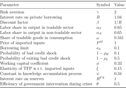
Some parameters are standard in the literature. The risk aversion parameter is set at γ = 2. The interest rate at which domestic agents can borrow from foreign investors is assumed equal to R = 1.04, while the discount factor is set to β = 1/R. We choose identical labor shares in the two sectors αT =αN = 0.65. The share of tradable goods in consumption is set to ω= 0.341 as in Durdu et al. (2009). The price of imported inputs
PM is normalized to 1 without loss of generality.
The parameters governing the financial frictions are set so that the version of the model without government intervention reproduces salient characteristics of developing countries. We set the borrowing limit κL equal to 0.1. This gives an average net foreign assets-to-GDP ratio of −16 percent, in the range of the values commonly observed in developing countries.18 The probability of experiencing a bad credit shock is set to 1 −ρH = 0.1 as in Jeanne and Ranci`ere (2011), while the probability of exiting an episode of financial turbulence is set to 1 −ρL = 0.5, following Alfaro and Kanczuk (2009). The fraction of imported inputs that has to be paid in advance φ is set to 0.33 to match an average working capital-to-GDP ratio of 6 percent. This is the same target as in Mendoza and Yue (2011).
To parameterize the process for the accumulation of knowledge we use the estimates provided by Coe et al. (1997). They find that the elasticity of TFP with respect to imports of machinery and equipment in developing countries is close to 0.3. They do not 17More precisely, we solve the model by iterating on the equilibrium conditions as proposed by Coleman
(1990).
18The precise value ofκ
H does not affect the simulations, as long as it is sufficiently high so that the
Table 1: Parameters
Parameter Symbol Value
Risk aversion γ 2
Interest rate on private borrowing R 1.04
Discount factor β 1/R
Labor share in output in tradable sector αT 0.65
Labor share in output in non-tradable sector αN 0.65
Share of tradable goods in consumption ω 0.341
Price of imported inputs PM 1
Borrowing limit κL 0.1
Probability of bad credit shock 1−ρH 0.1
Probability of exiting bad credit shock 1−ρL 0.5
Working capital coefficient φ 0.33
Elasticity of TFP w.r.t. imported inputs ξ 0.15 Constant in knowledge accumulation process ψ 0.34
Interest rate on reserves RF X 1
Efficiency of government intervention during crises θ 0.5
estimate which part of the effect can be attributed to spillovers that are not internalized by firms, so 0.3 is likely to be an upper bound for our parameter ξ. We take a pragmatic approach and set ξ = 0.15. The constant in the knowledge accumulation process ψ is set to 0.34, in order to match an average growth rate of 3 percent in the competitive equilibrium without government intervention.
The gross interest rate paid on reservesRF X is equal to 1. This gives a spread between private borrowing cost and the interest rate paid on reserves of 4 percent, in the range of the values considered by Rodrik (2006). We could not find good estimates for θ, the parameter that determines the efficiency of government intervention during crises. Hence, we somehow arbitrarily set it to 0.5. Our intuition is that our main results would not be affected by changes in the value of this parameter.
5.2
Results
We start by exploring how the foreign reserve policy affects the adjustment process of an economy that opens up to international capital flows. To capture the opening to international credit markets, we look at economies that start with no foreign debt (B0 =
0) and with no reserves (F X0 = 0) and we follow them during the transition to a steady
state in which foreign borrowing is allowed, but constrained by condition (9). We also assume that the economy starts in tranquil times (κ0 =κH).
We compare two different economies. First, we look at an economy in which the government does not intervene, that is in which χ = χW K = 0. Second, we consider an economy in which the government optimally chooses the parameters governing the foreign reserve policy,χandχW K. To compute the optimal policy we constructed grids forχand
χW K and then we searched for the combination of these two parameters that maximizes the expected lifetime utility of the representative household. Given our parametrization
the optimal policy is characterized by χ = 0.09, which implies that the government devotes 9 percent of the output of tradable goods to the accumulation of reserves during each tranquil period, and χW K = 1, which means that the government is willing to use up to its whole stock of reserves to intervene during crises.
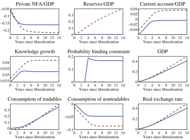
We derived forecast functions that describe the transition from financial autarky to the steady state with financial liberalization using the following procedure. For each model economy we performed 100000 stochastic simulations lasting for 15 periods each, taking as initial conditions B0 = F X0 = 0 and κ0 = κH. For each period we then averaged across all the simulations to obtain our forecast functions. Figure 4 shows the results of the experiment. To facilitate comparison, GDP, consumption of tradable goods, consumption of non-tradable goods and the real exchange rate are all expressed in percentage deviations from their first-period value in the equilibrium without government intervention.
Start by considering the solid lines, which describe the economy without government intervention. Upon opening to the international credit markets, the economy embarks in a period of accumulation of foreign debt that lasts for around five years, when the private net foreign assets-to-GDP ratio reaches its steady state value of−16 percent. The accumulation of foreign debt is the result of two forces. On the one hand, households living in an economy that is growing faster than the rest of the world, as we are implicitly assuming, have the desire to frontload their consumption stream and this pushes domestic agents to accumulate foreign debt. On the other hand, a high stock of foreign debt increases the negative impact of a bad credit shock on production of tradable goods. Because of this, domestic agents accumulate precautionary savings to self-insure against the risk of a bad credit shock and this puts a brake to the buildup of foreign debt. The counterpart to the process of debt accumulation are the high initial current account deficits, that progressively decrease until the current account-to-GDP ratio reaches its steady state value of −1 percent.
The first years following financial liberalization also see a progressive increase in the growth rate of the economy. This happens because foreign borrowing props up the con-sumption of tradable goods for a given amount of tradable goods produced. This gives an incentive to shift labor toward the production of non-tradable goods, which is higher during the first years after liberalization compared to its steady state value. As the econ-omy approaches its steady state, progressively more labor is allocated to the production of tradable goods, more intermediate inputs are imported and the growth rate of the economy increases until it reaches its steady state value.
Finally, during the first years after the opening to international credit markets the probability of experiencing a binding borrowing constraint is zero, because of the low stock of initial debt. As the stock of foreign debt increases, so does the probability of entering a financial crisis.
opti-0 2 4 6 8 10 12 14 −0.2 −0.15 −0.1 −0.05 Private NFA/GDP
Years since liberalization
0 2 4 6 8 10 12 14 −0.04 −0.02 0 0.02 0.04 Current account/GDP
Years since liberalization
0 2 4 6 8 10 12 14 0
0.2 0.4
GDP
Years since liberalization 0 2 4 6 8 10 12 14 0.025 0.03 0.035 0.04 Knowledge growth
Years since liberalization
0 2 4 6 8 10 12 14 0
0.1 0.2
Probability binding constraint
Years since liberalization
0 2 4 6 8 10 12 14 −0.1
−0.05 0
Consumption of nontradables
Years since liberalization 0 2 4 6 8 10 12 14 0 0.1 0.2 0.3 Consumption of tradables
Years since liberalization
0 2 4 6 8 10 12 14 0
0.2 0.4
Real exchange rate
Years since liberalization 0 2 4 6 8 10 12 14 0 0.1 0.2 0.3 Reserves/GDP
Years since liberalization
No intervention Optimal policy
Figure 4: Effects of financial liberalization. Notes: GDP, consumption of tradables, consumption of non-tradables and the real exchange rate are all expressed in percentage deviations from their first-period value in the equilibrium without government intervention. NFA refers to net foreign assets.
mal policy. After the opening to the international credit markets the government starts to accumulate foreign reserves at a fast pace. In fact, in the first fifteen years after financial liberalization the reserves-to-GDP ratio passes from 0 to almost 40 percent. Afterward, the reserves-to-GDP ratio keeps growing until it reaches its steady state value of 84 per-cent. Because of this policy, net capital inflows are lower compared to the laissez-faire equilibrium. Indeed, in steady state the current account-to-GDP ratio in the economy with policy intervention is 5 percentage points higher than in the economy without in-tervention.
Interestingly, the economy with government intervention posts higher current account surpluses despite higher accumulation of foreign debt from the private sector. The large buildup of private debt is driven by two effects. First, as discussed in section 4, pri-vate agents take on foreign debt to partly offset the impact of reserve accumulation on consumption. Second, in the economy with government intervention the incentives for private agents to build a stock of precautionary savings are weaker, because firms in the tradable sector anticipate that the government will supply working capital financing dur-ing crisis events. The result is that in steady state the private net foreign assets-to-GDP ratio is 5 percentage points lower compared to the economy without policy intervention.
Despite the reaction of private agents and because of the imperfect substitutability between private and public capital flows, the government policy succeeds in engineering a real exchange rate undervaluation that shifts productive resources out of the non-tradable sector and into the production of tradable goods.19 Moreover, the government
interven-tion during crises reduces to almost zero the probability of facing a binding borrowing constraint. These two effects lead to a higher use of imported inputs and to a faster growth rate of the economy compared to the equilibrium with no policy intervention. In fact, in steady state the growth rate of the stock of knowledge is 1 percent higher than under laissez-faire.
The model is thus able to replicate the negative correlation between growth and capital inflows observed in the data. Moreover, consistent with empirical evidence, the correlation is driven by the accumulation of foreign reserves from the public sector.
Figure 4 can also be used to illustrate the intuition underlying the impact on welfare of government interventions. During the first years after financial liberalization, con-sumption of tradable goods is lower in the economy with policy intervention compared to the laissez-faire equilibrium. This happens because the government appropriates trad-able goods from the private sector to finance the accumulation of reserves. However, the government policy also leads to faster growth and this explains why from year 9 on the consumption of tradable goods becomes higher in the equilibrium with policy intervention compared to the one without intervention. Hence, the government faces a trade-off be-tween lower consumption of tradable goods in the present, in exchange for faster growth and thus higher consumption of tradable goods in the future.
To describe the impact on welfare of different reserve management policies, we report the welfare gains that can be obtained from government intervention for an economy that undergoes financial liberalization. We compute the welfare gains of moving from the equilibrium with no intervention to a generic policy regimeias the proportional increase in consumption for all possible future histories that households living in the economy with no policy intervention must receive in order to be indifferent between remaining the no-intervention economy and switching to policy regime i. Formally, the welfare gain η
is defined as E0 " ∞ X t=0 βt((1 +η)C n t) 1−γ 1−γ # =E0 " ∞ X t=0 βtC i t1 −γ 1−γ # ,
where the superscriptsnandidenote allocations respectively in the economy with no pol-icy intervention and under a generic polpol-icy regimei. Since we want to look at economies that start from financial autarky we set the initial states to B0 = 0, F X0 = 0 and 19Notice that the undervaluation refers to the real exchange rate purged from the Balassa-Samuelson
effect. In absolute terms, the real exchange rate in the economy with policy intervention is undervalued compared to the laissez-faire equilibrium only during the first years after liberalization. Due to faster productivity growth in the tradable sector induced by reserve accumulation, the real exchange rate in the economy with government intervention eventually becomes more appreciated than in the economy with no intervention.
0 0.05 0.1 0.15 −1 −0.5 0 0.5 1 1.5
Consumption equivalent in percent
χ χWK = 0 χWK = 0.25 χWK = 0.5 χWK = 0.75 χWK = 1
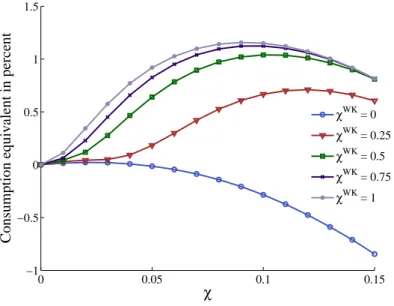
Figure 5: Welfare impact of policy interventions. Notes: χ is the fraction of tradable output devoted to reserve accumulation during tranquil times. χW K is the maximum amount of resources that the
government is willing to use during crisis events, expressed as a fraction of the start-of-period stock of foreign exchange reserves.
κ0 =κH.
Figure 5 presents the results of our welfare analysis by plotting the welfare gains as a function of the resources employed to accumulate reserves during tranquil times χ, for different intensities of the intervention during crises χW K.
The first thing to notice is that the welfare gains from policy intervention are quantita-tively significant. For instance, the optimal policy delivers welfare gains above 1 percent of permanent consumption equivalent. Moreover, the bulk of the welfare gains seems to come from the ability to provide liquidity to firms during crises. This can be seen from the large welfare differences between the economy with no intervention during crises (χW K = 0) and those in which the government does intervene to provide liquidity during periods of financial turbulence (χW K > 0). In addition, under the welfare maximizing rule reserves are accumulated at a fast pace, since 9 percent of the output of tradable goods is devoted to the accumulation of reserves each tranquil period.
Interestingly, some welfare gains, albeit small, can be obtained through the accumu-lation of foreign exchange reserves also when they cannot be used to intervene during crises. This can be seen by looking at the χW K = 0 line, which reaches its maximum corresponding to a consumption equivalent of 0.02 percent when χ= 0.02. Thus reserve accumulation can be a welfare enhancing policy also when reserves cannot perform their traditional role of liquidity provider during financial crises.