Deep Reinforcement Learning in Medical Object Detection and Segmentation

Scholarship@Western

Scholarship@Western

11-11-2020 2:00 PM

Deep Reinforcement Learning in Medical Object Detection and

Deep Reinforcement Learning in Medical Object Detection and

Segmentation

Segmentation

Dong Zhang, The University of Western Ontario

Supervisor: Shuo Li, The University of Western Ontario

A thesis submitted in partial fulfillment of the requirements for the Master of Engineering Science degree in Biomedical Engineering

© Dong Zhang 2020

Follow this and additional works at: https://ir.lib.uwo.ca/etd

Part of the Bioimaging and Biomedical Optics Commons, and the Biomedical Commons

Recommended Citation Recommended Citation

Zhang, Dong, "Deep Reinforcement Learning in Medical Object Detection and Segmentation" (2020). Electronic Thesis and Dissertation Repository. 7423.

https://ir.lib.uwo.ca/etd/7423

This Dissertation/Thesis is brought to you for free and open access by Scholarship@Western. It has been accepted for inclusion in Electronic Thesis and Dissertation Repository by an authorized administrator of

Medical object detection and segmentation are crucial pre-processing steps in the clinical workflow for diagnosis and therapy planning. Although deep learning methods have achieved considerable performance in this field, they impose several shortcomings, such as computa-tional limitations, sub-optimal parameter optimization, and weak generalization. Deep rein-forcement learning as the newest artificial intelligence algorithm has great potential to address the limitation of traditional deep learning methods, as well as obtaining accurate detection and segmentation results. Deep reinforcement learning has a cognitive-like process to propose the area of desirable objects, thereby facilitating accurate object detection and segmentation. In this thesis, we deploy deep reinforcement learning into two challenging and representative medical object detection and segmentation tasks: 1) Sequential-Conditional Reinforcement Learning (SCRL) for vertebral body detection and segmentation by modeling the spine anatomy with deep reinforcement learning; 2) Weakly-Supervised Teacher-Student network (WSTS) for liver tumor segmentation from the non-enhanced image by transferring tumor knowledge from the enhanced image with deep reinforcement learning. The experiment indicates our methods are effective and outperform state-of-art deep learning methods. Therefore, this thesis improves object detection and segmentation accuracy and offers researchers a novel approach based on deep reinforcement learning in medical image analysis.

Keywords: Deep reinforcement learning, Medical object detection and segmentation, Ver-tebral body segmentation, Liver tumor segmentation, Teacher-student framework

Automatic medical object detection and segmentation based on artificial intelligence as computer-assisted-diagnosis tools are significant for clinicians in the disease diagnosis and treatment planning. Medical object detection and segmentation distinguish the object of interest from the medical image, which provides clinicians with the location, shape, and size of the object, thereby assisting clinicians to make a decision. Deep learning methods have achieved consid-erable performance in this field by leveraging convolutional neural networks. However, as the development of deep learning, it also imposes some limitations and its accuracy in some tasks cannot meet clinical expectations. In this case, this thesis seeks to employ deep reinforcement learning to address the limitations of deep learning methods and obtain accurate medical ob-ject detection and segmentation. Particularly, this thesis deploys deep reinforcement learning in vertebral body segmentation, where the newly-proposed Sequential-Conditional Reinforce-ment Learning (SCRL) models the spine anatomy as a sequential decision-making process and segments vertebral bodies along the spine. In another project, this thesis deploys deep rein-forcement learning into a more challenging task. Particularly, this thesis proposes the Weakly-Supervised Teacher-Student network (WSTS) to address liver tumor segmentation from the non-contrast-enhanced image. WSTS leverages deep reinforcement learning to transfer tumor spatial information for the contrast-enhanced image in the training stage, which plays as guid-ance to determine the liver tumor location in the non-contrast-enhguid-anced image. The results of the above two methods outperform the results of existing deep learning methods. The success of proposed methods in medical object detection and segmentation indicates the deep rein-forcement learning can be a reliable computer-assisted-diagnosis tool and benefit to clinicians.

The following thesis consists of 2 manuscripts and both of them have been submitted to a peer-reviewed journal. Dong Zhang, as the first author, was a significant contributor to both studies, framework propose, validation experiment design and implementation, data analysis, and manuscript preparation. Dr. Shuo Li, as the principal investigator and supervisor, provided guidance and aided in the study conception, direction, and data acquisition. Additionally, Dr. Li was responsible for the approval and submission of the manuscripts.

Chapter 2 is an original research article entitled, ”Sequential Conditional Reinforcement Learn-ing for Automatic Vertebral Body Detection and Segmentation”. This manuscript was submit-ted to the peer-reviewed journalMedical Image Analysis. This manuscript was co-authored by Dong Zhang Bo Chen, and Shuo Li.

Chapter 3 is an original research article entitled, ”Weakly-Supervised Teacher-Student Network for Liver Tumor Segmentation from Non-enhanced Images”. This manuscript was submitted to the peer-reviewed journal Medical Image Analysis. This manuscript was co-authored by Dong Zhang and Shuo Li.

I would like to thank my supervisor, Dr. Shuo Li for his support and guidance in my research and life. Thank you for teaching me research skills, including academic paper writing and scientific oral presentation delivering. I am grateful you reviewed my manuscripts line by line and feed-backed professional comments. Thank you for pushing me tirelessly to work hard and helping me through these fulfilling two years. I am also grateful for the philosophy of life you told me beyond research when I was in frustrations.

I am thankful to have Dr. James Lacefield and Dr. Ali Khan as members of my advisory com-mittee. Thank you for engaging in my research and for guiding me in the right direction. Your constructive criticisms and words of encouragement have been significant in the development of my research and towards accomplishing my goals.

The past and present members of the Digital Imaging Group of London lab have been im-mensely supportive providing an invaluable environment to adaptive the abroad life, acquire a wealth of knowledge, and develop as a researcher. To Clara Tam, thank you for being a great friend and colleague. Thank you for helping me to adapt to the new life and study when I first time left my motherland and came to Canada to study alone. Thank you for being there as a teacher to give me advice and guidance patiently, and for imparting your experience to me. To Dr. Chenchu Xu, thank you for being a sincere friend and roommate. Thank you for spending the extra time to aid me in my research. Thank you for putting up with my irritability when I encountered setbacks and teaching me to be pliable but strong. To Dr. Rongchang Zhao, thank you for providing comments to the logical sequence and structure of my papers. To Dr.Liyan Lin, Dr. Rongjun Ge, Dr. Shumao Pang, Mr. Yuqi Qian, thank you for sharing technical knowledge and writing experience.

Most importantly, I would like to thank my parents Zhilu and Xurui. Your support and encour-agement have been essential to my success. Although thousands of miles exist between us, you were always my backing to inspire me to do my best, and to have the courage to tackle anything that comes my way.

The computing resources provided through Niagara, funded by the Ontario Government and the Federal Economic Development Agency for Southern Ontario, and local resources pro-vided by Dr. Jaron Chong have been integral to the completion of my research. I would like to express my sincere gratitude and appreciation to them for making my research possible. Computations using the Niagara platform were performed using the data analytics Cloud at the

Lastly, I would like to express my deepest gratitude to the various sources of funding that I received throughout my graduate studies. I acknowledge funding support from the China Scholarship Council, School of Biomedical Engineering at The University of Western Ontario, and The University of Western Ontario.

Abstract

ii

Lay Summary

iii

Co-Authorship Statement

iv

Acknowledgements

v

List of Figures

xi

List of Tables

xiv

List of Abbreviations

1

CHAPTER 1

1

1 INTRODUCTION 1

1.1 Overview . . . 1

1.2 Medical object detection and segmentation from images . . . 2

1.2.1 Medical image acquirement . . . 2

1.2.2 Medical object detection and segmentation . . . 4

1.3 Deep learning (DL) . . . 6

1.3.1 Convolutional neural network . . . 6

1.3.2 Loss function & Back propagation . . . 10

1.3.3 Types of learning . . . 10

1.4 DL in medical object detection and segmentation . . . 11

1.5 Deep Reinforcement Learning (DRL) . . . 13 1.5.1 Reinforcement Learning (RL) . . . 13 Value-based methods . . . 15 Policy-based methods . . . 15 Actor-Critic method . . . 16 1.5.2 DRL algorithms . . . 16 Deep Q-learning . . . 16 Soft Actor-Critic . . . 18

1.5.3 The great potential of DRL in medical object detection and segmentation 18 1.6 Thesis objective . . . 19

References . . . 20

CHAPTER 2

24

2.1.1 Deep reinforcement learning . . . 27

2.1.2 Method overview . . . 29

2.1.3 Contributions . . . 30

2.2 Background review . . . 30

2.2.1 Deep Reinforcement Learning . . . 30

2.3 Method . . . 32

2.3.1 Anatomy-Modeling Reinforcement Learning (AMRL) . . . 33

Multi-Channel State . . . 34

Continuous-Transforming Action . . . 36

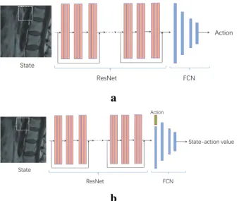
Agent network . . . 37

Consequence-Oriented Reward Function (CORF) . . . 38

Adaptive-Sampling Experience Replay (ASER) . . . 40

2.3.2 Fully-Connected Residual Neural Network (FC-ResNet) . . . 41

2.3.3 Y-Shaped Network (Y-Net) . . . 42

2.4 Data and experiments . . . 43

2.4.1 Data acquisition . . . 43

2.4.4 Stated-related hyperparameter setting . . . 45

2.4.5 Training strategy for SCRL . . . 45

2.4.6 Implementation details . . . 45

2.4.7 Experimental setting . . . 47

Detection evaluation for FC-ResNet . . . 47

Segmentation evaluation for Y-Net . . . 48

Classification evaluation for Y-Net . . . 49

Attention-focusing evaluation for AMRL . . . 49

2.4.8 Results and discussion . . . 50

Detection result . . . 50

Segmentation result . . . 54

Classification result . . . 58

Effectiveness of AMRL for attention-focusing . . . 59

References . . . 62

CHAPTER 3

67

3.2 Motivations in the WSTS . . . 72

3.2.1 Motivation for the DDRL . . . 72

3.2.2 Motivation for the USSE . . . 73

3.3 Related work . . . 74

3.3.1 Existing work . . . 74

3.3.2 Algorithm background . . . 75

Deep reinforcement learning . . . 75

Actor-Critic method . . . 76

Experience replay . . . 77

3.4 Method . . . 77

3.4.1 Teacher Module . . . 78

Dual-strategy DRL (DDRL) . . . 79

Uncertainty-Sifting Self-Ensembling (USSE) . . . 83

3.4.2 Student module . . . 85

3.5 Experiment . . . 87 3.5.1 Data acquirement . . . 87 3.5.2 Implementation details . . . 88 3.5.3 Evaluation criteria . . . 88 3.5.4 Experimental setting . . . 90 Control experiments . . . 90 Ablation experiments . . . 91 Inter-comparison experiments . . . 91 3.5.5 Experimental result . . . 92 Comprehensive analysis . . . 92

Evaluation of control experiments . . . 93

Evaluation of ablation experiments . . . 94

Evaluation of inter-comparison . . . 96

References . . . 100

CHAPTER 4

106

4.2 Summary and Conclusions . . . 107

4.3 Significance and Impact . . . 108

4.4 Limitations . . . 108

4.4.1 Study Specific Limitations . . . 108

4.4.2 General Limitation . . . 109

4.5 Future Directions . . . 109

4.5.1 End-to-end framework design . . . 109

4.5.2 Three-dimensional (3D) image segmentation . . . 110

4.5.3 Extension to other tasks . . . 110

APPENDIX

111

Curriculum Vitae

121

Figure 1.1 Precession of protons in a static magnetic field. ... 2

Figure 1.2 Workflow of Deep learning ... 6

Figure 1.3 An artifical neuron model ... 7

Figure 1.4 A convolution process... 8

Figure 1.5 Examples for convolution-based feature extraction ... 8

Figure 1.6 An example of pooling process ... 9

Figure 1.7 Reinforcement Learning ... 14

Figure 1.8 Deep Q-learning ... 17

Figure 1.9 Experience replay ... 18

Figure 2.1 Challenges in vertebral body detection and segmentation... 26

Figure 2.2 The potential of deep reinforcement learning ... 27

Figure 2.3 The principle of DRL ... 28

Figure 2.4 Comparison between our method and traditional methods... 29

Figure 2.5 Framework of SCRL ... 32

Figure 2.6 Anatomy-Modeling Reinforcement Learning ... 34

Figure 2.7 Multi-Channel State ... 35

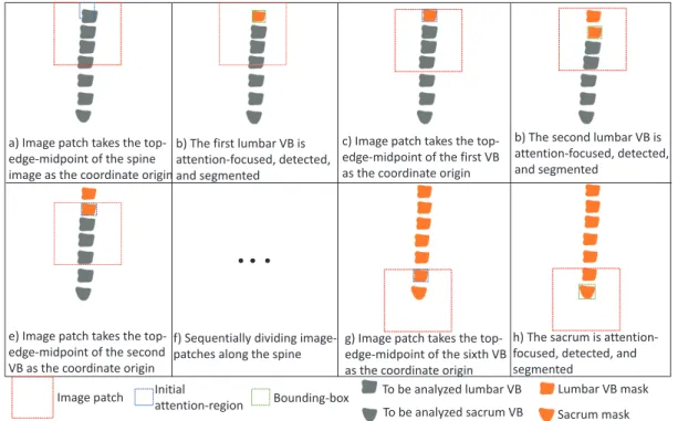
Figure 2.8 Image-patch and attention-region initialization ... 36

Figure 2.9 Continuous-Transforming Action ... 37

Figure 2.10 Architectures of networks in AMRL ... 38

Figure 2.11 The network architecture of Y-Net ... 42

Figure 2.13 Detection visualization of SCRL ... 50

Figure 2.14 Detection performance in each kind of VBs ... 51

Figure 2.15 Visualization examples of VB detection for existing methods ... 53

Figure 2.16 Segmentation visualizations of SCRL... 55

Figure 2.17 Segmentation performance on each kind of VBs ... 55

Figure 2.18 ROC and PRG Curves... 56

Figure 2.19 Visualization examples of VB segmentation for existing methods ... 57

Figure 2.20 Effectiveness of AMRL for attention-focusing... 60

Figure 3.1 The clinical significant of proposed method ... 68

Figure 3.2 Challenges in tumor segmentation ... 69

Figure 3.3 The potential of the teacher-student framework ... 70

Figure 3.4 The workflow of WSTS... 71

Figure 3.5 Motivation of DRL... 73

Figure 3.6 Framework of WSTS ... 78

Figure 3.7 The architecture of DDRL ... 80

Figure 3.8 The composition of USSE ... 83

Figure 3.9 Tumor segmentation visualization in WSTS ... 92

Figure 3.10 ROC curves ... 95

Figure 3.11 Ablation experimental result related to the DRL method... 96

Figure 3.12 Ablation experimental result related to the semi-supervised method ... 97

Figure A.1 Back propagation ... 111

Figure D.1 Location and size distributions of the first VB ... 117

Figure D.2 Extreme examples for the start image-patch ... 117

Figure D.3 The location changes between adjacent VBs ... 118

Figure D.4 The size changes between adjacent VBs... 118

Figure F.1 The network architectures in DDRL ... 120

Table 2.1 Training configurations of the SCRL network ... 47

Table 2.2 Performance comparison of SCRL with existing state-of-art methods... 51

Table 2.3 Detection comparison among AMRL, Y-Net, and FC-ResNet ... 54

Table 2.4 Segmentation performance comparison between Y-Net and U-Net... 56

Table 2.5 Attention accuracy under different hyperparameter-settings... 59

Table 3.1 Control experimental result ... 93

Table 3.2 Inter-comparison experimental result ... 98

2D Two-Dimensional

AC Actor-Critic

AMRL Anatomy-Modeling Reinforcement Learning ASER Adaptive-Sampling Experience Replay AUC Area Under the Curve

BP Back Propagation

CNN Convolutional Neural Network

CORF Consequence-Oriented Reward Function

DL Deep Learning

Dice Dice coefficient

DRL Deep Reinforcement Learning DDRL Dual-strategy DRL

FC-ResNet Fully Connected Residual Neural Network HD HausdorffDistance

IA Image Accuracy

IDR Identification Rate IoU Intersection over Union KAP Cohen Kappa Coefficient

MA Mean Accuracy

MRI Magnetic Resonance Imaging

MSE Mean Squared Error

Loc-Err Localization-Error ResNet Residual Network PA Pixel-level Accuracy ResNet Residual Neural Network

RF Radio Frequency

ROC Receiver Operating Characteristic RoI Region of Interest

SCRL Sequential Conditional Reinforcement Learning SAC Soft Actor-Critic

T Tesla

TCH-ST Teacher-Student framework

TE Time to Echo

TR Repetition Time

USSE Uncertainty-Sifting Self-Ensembling

VB Vertebral Body

WSTS Weakly-Supervised Teacher-Student network Y-Net Y-shaped Network

CHAPTER 1

This chapter provides a general introduction to medical object detection and segmentation, as well as concepts about deep learning and deep reinforcement learning. A literature re-view of current development and challenges of deep learning in medical object detection and segmentation are included in this chapter. The motivation and objectives of applying deep rein-forcement learning algorithms in medical object detection and segmentation will be presented.

1

INTRODUCTION

1.1

Overview

Medical object detection and segmentation via Artificial Intelligence (AI) methods are vital roles in computer-aid diagnosis (CAD) to assist radiological experts in clinical diagnosis and treatment planning [1]. Image object detection and segmentation extract the region of interest (ROI), divide a medical image into different areas in pixel-level based on a specified require-ment, such as segmenting body organs/tissues in the medical applications for border detec-tion, tumor detection/segmentation, and mass detection[2]. Nowadays, the vast investment and development of medical imaging modalities such as microscopy, X-ray, ultrasound imaging, magnetic resonance imaging (MRI), computed tomography (CT), and positron emission to-mography (PET) generate a large amount of medical image data, which attracts researchers to explore AI methods such as Deep Learning (DL) to develop automatic medical object de-tection and segmentation methods. Applying AI methods to address medical object dede-tection and segmentation has several advantages in CAD: 1) Improving diagnosis efficiency. With the support of high-performance computers, the speed of AI methods detecting and segmenting the medical object from medical images is dozens or even hundreds of times faster than manual la-beling by radiologists. AI methods thus speed up the diagnosis process and improve diagnosis efficiency. 2) Increasing the diagnosis accuracy. AI methods process and segment the medical image according to the image content objectively, which avoids inconsistent results caused by observer subjectivity in manual segmentation. AI methods thus increase the diagnosis accu-racy compared with manual methods. 3) Reducing the diagnosis cost. AI methods process everything with computers and output the segmentation result automatically. AI methods get rid of the need for experienced radiologists to some extent, which reduces the diagnosis cost for some developing countries with poor medical conditions.

1.2

Medical object detection and segmentation from images

1.2.1

Medical image acquirement

The main type of medical images focused on in this thesis is MRI, which is referred to as cross-sectional slice images as it corresponds to what an object would express if it was sliced open along a special plane. MRI images thus can display detailed information on the anatomy inside the human body.

MRI images are generated by the exchange of radio frequency (RF) energy between the imag-ing system and a patient’s body. This is possible because the most abundant hydrogen atom (protons) within human tissue has unique magnetic properties. More specifically, a proton pos-sesses an innate spin angular momentum rotating about its axis at a constant rate [3–7]. When a strong static external magnetic field is applied, the protons’ rotational axes will change from free to align with the magnetic field. Since protons possess an angular momentum, they will precess about the applied field or rotate perpendicularly [8].

The proton’s precession rate is proportional to the strength of the magnetic field (see Fig. 1.1), which is expressed by the Larmor (resonance) frequency equation:

ωo =

γBo

2π (1.1)

Whereωois the Larmor frequency expressed in megahertz (MHz),Bois the main magnetic field

(in Tesla), andγis the gyro-magnetic ratio expressed in radian per second per tesla (rad·s-1T-1) or MHz/T for ₂γ_π [3, 4]. x y z BO RF

When the MRI imaging acquisition procedure starts, the operator introduces an RF pulse to place the protons into a strong magnetic field, which aligns spinning protons with long axis (parallel/antiparallel).

When the protons’ precessing frequency matches the applied RF pulse’s frequency, the pro-tons will begin to resonate and absorb some of the energy from the RF pulse, stimulating them into an excited state, which also has an increase in electromagnetic energy. When the operator removes the RF pulse, the protons in an excited state will realign with the magnetic field and re-lease the absorbed electromagnetic energy along the way. This process is known as relaxation. The transmitted electromagnetic energy is then captured by a receiver in the MRI scanner to reconstruct into the MR images.

Because varying tissues in the internal structure of the body contain varying amounts of water, more specifically, the concentration of protons. After the applied RF pulse is removed, MRI detects the emission of the excess energy from the protons to automatically distinguish the in-tensities of different tissues in the internal structure of the body.

Therefore, the relaxation time (or rate) is the most important factor to generate contrast in different kinds of tissues in the MRI imaging system. It is worth mentioning that the image quality is determined by the intensity of the RF signal.

There are two types of relaxation times T1 (longitudinal relaxation time) and T2 (transverse relaxation time) in MRI. T1 is the time-constant for the spinning protons to realign with the external magnetic field. That is to say, the time it takes for the longitudinal signal to regain 63% of its magnetization value. T2 is the relaxation time-constant for excited protons to lose phase coherence with each other [4, 5, 9]. That is to say, the time it takes for the transverse magnetization to decay to 37% of its original value [10].

MRI acquires image sequences by varying the RF pulses, based on the T1 and T2 relaxation to enhance the quality of select tissues. The repetition time (TR) is the time between successive pulse sequences applied to the same image slice[4, 5, 9]. The time to echo (TE) is the time between the delivery of an RF pulse and receiving the signals emitted from the patient’s body, which are referred to as echoes[4, 5, 9].

MRI sequences generate T1-weighted and T2-weighted scans based on the intrinsic T1 and T2 relaxation properties. T1-weighted sequences have shorter TR and TE times, whereas

T2-weighted have longer TR and TE times[4, 5, 9]. T1-T2-weighted images emphasize T1 relaxation, while T2W emphasise T2 relaxation. Fat has Short T1 and medium T2. So that fat shows up bright in T1-weighted and intermediate in T2-weighted. Fluid has Long T1 and T2, so that fluid shows up dark in T1-weighted and bright on T2-weighted.

1.2.2

Medical object detection and segmentation

Medical object detection and segmentation are complex and critical steps in the field of medi-cal image processing and analysis. Their purposes are to detect the regions with certain special meanings (such as lesions and vertebral bodies) from medical images and to classify pixels in the regions into desirable objects, providing a reliable basis for clinical diagnosis and pathol-ogy research to assist doctors to make a more accurate diagnosis [11]. The clinical significance of medical object detection and segmentation is (take radiation therapy as an example) [12]: (1) study anatomical structures; (2) identify regions of interest (i.e., locate tumors, lesions, and other abnormal tissues); (3) measure the volume of desirable objects; (4) Observe the growth of the tumor or the decrease of the tumor volume during treatment, and provide assis-tance for the planning and treatment before treatment; (5) Calculation of radiation dose. To address the medical object detection and segmentation, several methods have been proposed. Traditional medical object detection and segmentation methods involve thresholding, edge de-tection, region-based, and active contour model methods.

The basic principle of the thresholding method is to calculate one or more thresholds based on the grayscale characteristics of the image, and then compare the image pixel by pixel with the threshold, and finally divide each pixel into the correct category. The thresholding method is based on an assumption of the grayscale image: the grayscale values between adjacent pixels in the target or background are similar, but the pixels of different targets or backgrounds are different in grayscale, which is reflected on the image histogram is that: different targets and backgrounds correspond to different peaks. The selected threshold should be located in the val-ley between the two peaks to separate the peaks. The disadvantage of the thresholding method is that it is not suitable for multi-channel images and images with similar feature values. It is difficult to obtain accurate object detection and segmentation result where there is no obvious gray difference in the image or there is a large overlap in the gray value range of each object. In addition, because it only considers the gray information of the image without considering the spatial information of the image, threshold segmentation is very sensitive to noise and gray unevenness. Several methods of threshold selection are histogram thresholding method [13], iterative thresholding method [14], and adaptive thresholding method [15]. The most famous

one is the Otsu threshold method (OTSU) [15], which obtains segmentation results by maxi-mizing the variance between classes.

The basic principle of edge detection methods is to achieve segmentation by detecting edges containing different regions. One of the main assumptions of this method is that the change in pixel gray value on the edge between different regions is usually relatively strong. Therefore, according to this assumption, the zero feature of the second derivative of the image and the maximum value of the first derivative can be used to determine whether it belongs to the pixel on the edge. The edge detection method has the advantages of accurate positioning and fast speed, but it cannot guarantee the continuity and closure of the edge and is quite sensitive to noise. Common edge detection algorithms are Canny [16] [17], Sobel [18], and Laplacian [16].

The region-based method is based on directly searching for image blocks, and includes region growth and region separation and merging technologies [19]. The regional growth technique first determines a seed point for each region to be divided as the starting point for growth, and then merges the pixel points in the neighborhood of the seed point that are the same or similar to the point into the area where the seed point is located, and updates the seed point to repeat The above process until no new pixels that meet the conditions are merged. The whole pro-cess starts from the seed point, and finally gets the entire area, and then finishes the detection and segmentation task. Splitting and merging can be regarded as the inverse process of region growth. It starts from the whole and continuously splits to obtain each sub-region, and then gradually merges the target regions to achieve the purpose of detection and segmentation. The region-based method is suitable for smooth and uniform images, and the algorithm is simple and the calculation is fast. However, it requires manual selection of seed points, and has poor anti-noise ability. For high-noise, non-uniform medical images, the detection and segmentation results are often poor.

The active contour model uses curve fitting to achieve the purpose of detection and segmen-tation. First, the contour information is initialized, and then the image information is used to estimate the energy model. The energy is minimized to guide the contour change and gradu-ally approach the target edge to obtain the segmentation result. Snake model [20] is a typical active contour model method, which makes the curve gradually close to the edge under the joint action of image information and the curve itself. It has the advantages of direct interac-tion with the model, compact model expression and fast implementainterac-tion speed, but it is very sensitive to the curve initialization and it is difficult to deal with changes in the model topology.

However, with the rapid development of AI, leveraging the artificial neural networks to detect and segment medical objects from images is becoming more and more popular. Compared with traditional methods, AI methods achieve higher precision, faster speed, and higher reliability.

1.3

Deep learning (DL)

Deep Learning (DL) is a subset of machine learning in AI, which imitates the human brain working process to learn to build a non-linear mapping between inputs and the desired output. The learning (or training) procedure of DL is an iterative process (as shown in Fig 1.2): a convolution neural network(CNN) predicts an output according to the input(forward propa-gation); then aloss functionevaluates the error between the predicted output and the desired output; DL adjusts the CNN’s parameters through back propagation based on the error to enable its prediction to approach the desired output in next forward propagation. Repeating the above training process, after the error between the predicted output and the desired output is less than a threshold, DL is able to predict the output for a new same category input.

Forward propagation

Back propagation

Input Output

Loss function

Figure 1.2.The workflow of deep learning.

1.3.1

Convolutional neural network

Convolutional neural network (CNN) [21] assembles low-level features to build abstract high-level features, thereby finding the distributed feature representation in the data. CNN is origi-nated from the artificial neural network, which models human brain neuron network from the perspective of information processing.

Artifical neural network takes neuron as the basic unit and constructs network architecture via the interconnection between neurons. As shown in Fig 1.3, a neuron takes several input

…. …. x1 x2 xn ʘ1 ʘ2 є ɽ ʍ _y

Figure 1.3. An artifical neuron model.

signalsxi and outputs a weighted signal with a bias, which can formulated as follows:

y=

n

X

i

ωi∗ xi+ (1.2)

Thus a network made up by several neurons can be deployed to building the mapping between an input and an output by learning suitable weights and biases. In imaging processing, convo-lutions are deployed as neurons to build neural networks, i.e., Convolution Neural Networks (CNNs). Compared with building neurons with pixels, CNN reduces the number of connection weights in neural networks to a range that can be handled in practice. In detail, CNN consists following three layers:

Convolution Layer extracts various image characteristics (such as boundary, texture, and color) through convolution and Stacks convolution sequentially as a hierarchy pyramid to achieve the high-level feature extraction. Convolution is a common mathematical operation in a signal process. A convolution to a matrix is shown in Fig 1.4, the 5∗5 square in the left of the figure is regarded as the image input. The 3∗3 white square in the middle with the numbers 1, 0, -1, and -2 are the convolution kernels. The convolution kernels have a step size of 1. The sequence moves from the up left corner of the original input to the bottom right corner, and the convolution kernel moves a total of 9-times. The position of the nine time corresponds to the corresponding blue 3 * 3 grid on the right. The number in the grid is the convolution value (here is the result of multiplication and accumulation of the elements in the area covered by the convolution kernel). After 9 movements are calculated, the new matrix of 3 * 3 on the right is the calculation result of this convolution.

In the actual calculation process, the input is an original image and a filter (a set of fixed weights, which is the actual meaning of the convolution kernel mentioned above). After the inner product is obtained, new two-dimensional data is obtained. Different filters will get dif-ferent output data, such as contour and color depth. If you want to extract different features of the image, you need to use different filters (convolution kernel) to extract the specific informa-tion you want about the image. Fig 1.5 shows the process of convoluinforma-tion in a convoluinforma-tional layer. Through the convolution operation of two different convolution kernels above and

be-Figure 1.4. A convolution process. The left matrix represents an image before the convolution, the middle matrix represents the convolution kernel, and the right matrix represents the matrix after the convolution.

low, the features of different images can be extracted. The new two-dimensional information will be used as the input of the next convolutional layer in the CNN network. That is, when the next convolutional layer is calculated, the image on the right will be used as the original input image. The shallower (low-level) convolutional layer has a smaller perception domain and learns the characteristics of some local regions; the deeper (high-level) convolutional layer has a larger perception domain and can learn more abstract features. These abstract features are less sensitive to the size, position, and orientation of objects, thereby helping to improve recognition performance.

Figure 1.5. Two examples to show different convolution kernels result in different feature maps.

The feature obtained after convolution is a static feature of the image, which means that a fea-ture useful in one area is likely to be useful in another. At this time, we can use the statistical characteristics of the region to describe the region’s information. At the same time, consider-ing that the model needs to have a certain degree of robustness to translation and rotation in practical applications, it is beneficial to enhance the robustness by describing the region fea-tures rather than the region itself. There are generally two types of pooling operations, one is average pooling and the other is maximum pooling. The maximum pooling operation is using a 2×2 filter, the maximum is to find the maximum value in each region, here the step size is 2, and finally extract the main features in the original feature map. The method of average pool-ing layer is to sum each 2 ×2 area element and divide by 4 to get the main features, Fig. 1.6 illustrates the maximum pooling.

1 Ͳ1 2 1 Ͳ1 2 1 Ͳ2 2 Ͳ1 Ͳ1 0 1 1 0 1 0 0

Feature map Feature map

Maximum Pooling

1 2 1 2

1 1 1 1

1HZIeature map 1HZIeature map

Figure 1.6. An example of pooling process. After the pooling, the new feature map keeps the important information of the original feature map but reduces its size.

Fully Connected Layeris the ”classifier” in CNN. If the operations of the convolutional layer and the pooling layer are to map the original data to the hidden layer feature space, the fully connected layer plays the role of mapping the learned feature representation to the sample’s label space. In detail, a fully connected layer flats the 2-dimensional feature into a single vec-tor of values, each representing a probability that a certain feature belongs to a label. When multiple fully connected layers are superimposed, a nonlinear relationship between object char-acteristics and object categories can be constructed.

1.3.2

Loss function & Back propagation

Loss function and back propagation usually work together to enable the CNN prediction to approach the ground-truth. Particularly, loss function measures the distance between the CNN prediction and the ground-truth, back propagation adjusts the CNN parameters based on the loss function value to reduce the distance between the prediction and ground-truth.

Loss function contains following types in this thesis: MSE loss, i.e., mean square error, which is usually deployed to measure the segmentation and regression quality. MSE loss calculates the average squared difference between the estimated values and the actual value. If the vector (or matrix) has N prediction ˆyand corresponding true valuey, MSE loss can be formulated as follow: MS E = 1 N N X i=1 (yi−yˆi)2 (1.3)

Dice losswhich is usually deployed in small object segmentation evaluation. Dice loss calcu-lates the Dice coefficient between the ground-truth and the prediction. Assuming there are a 2D segmentationXand a ground-truthY, Dice loss is:

Dice= 2|X∩Y|

|X|+|Y| (1.4)

Different from MSE loss, which focuses on the overall performance, Dice loss only pays at-tention to the segmentation performance on the desirable object. Thus Dice loss is usually employed in small object segmentation to improve the result precision.

Back propagation (BP) is the most common and effective method to train the ANN. The main principle of BP is:

1) Inputting the training data into an ANN and getting the output, which is forward propagation. 2) Because there is an error between the output of ANN and the true label, calculating the error and back-propagating the error to every layer until the input layer.

3) During back-propagation, adjusting the ANN parameters in every layer.

4) Repeating the above procedure iteratively until the error between the output and the true label is less than a tolerance range, which is convergence. The complete formula derivation of BP is shown in Appendix. A.

1.3.3

Types of learning

According to the provided label in a dataset, DL algorithms can be divided into the following categories: fully-supervised learning, semi-supervised learning, and weakly-supervised

learn-ing.

Fully-supervised learning: In the given dataset, the input and label are one-to-one correspon-dence. Thus fully-supervised learning algorithms aim to train a mapping from the input to the corresponding label. For instance, the label for binary segmentation in the fully-supervised learning is a mask where every pixel is 1 or 0 to indicate the class (foreground or background) of this pixel in the input image. Fully-supervised learning algorithms are the most common training method because theoretically their performance is the best and their training proce-dures are the simplest.

Unsupervised learning: In the given dataset, there is only input data without any labels. In this case, unsupervised learning algorithms learn the inherent structure of the data from discov-ering specific patterns through repetitive experiences, such as the gray scale difference between the tumor and the normal tissue. Unsupervised learning algorithms are only suitable for some specific tasks where the data has distinguishable inherent patterns.

Semi-supervised learning:In the given dataset, only partial inputs have corresponding labels, the other partial inputs have unknown labels (or no labels). While semi-supervised learning algorithms aim to make full use of all data in the dataset to learn a mapping from the input the correct label. Generally, semi-supervised learning algorithms are usually used for some tasks where the label is difficult to be annotated.

Weakly-supervised learning:In the dataset, every input has a corresponding weak label. The weak label means it provides less information compared with the label. Weakly-supervised learning algorithms aim to map the input to a more specific label. For instance, in a pixel-level object segmentation tasks, the provided weak label is bounding-boxes of desirable objects. Here, the label is not so accurate that indicates the class of every pixel, but it indicates the ob-ject location and size. Thus, the weakly-supervised learning algorithms try to take advantage from these weak labels to exploit the input inherent features, thereby accomplishing the task.

1.4

DL in medical object detection and segmentation

DL achieves great performance in medical object detection and segmentation, but it also ex-poses many limitations along with the development. Compared with traditional machine learn-ing methods which extract a limited number of image features with hand-crafted algorithms,

DL leverages CNN to extract numerous image features and fully connected layers to regress the object location. More importantly, DL adjusts the parameters of CNN and fully connected layers through BP to extract more proper image features and reduce the distance between its prediction and the ground-truth, thereby achieving great detection and segmentation results. However, DL also has several limitations and cannot address some challenging medical object detection and segmentation tasks.

1.4.1

DL methods for medical object detection and segmentation

FCN methods are the pixel-to-pixel network in which every layer is a convolutional layer, they input the medical image and output the same size segmentation directly. The most fa-mous FCN method in medical image segmentation is U-Net[22]. Its encoder (downsampling) - decoder (upsampling) structure is a remarkable design method. Particularly, U-Net extracts high-level features from the low-level features through the encoder, and restores the size of the feature to the same size as the input, thereby achieving pixel-level segmentation. More-over, U-Net also employs skip-connections between the encoder and the decoder to convey the low-level features from the encoder to the decoder directly, which avoids feature losing in the downsampling effectively. There are many new convolutional neural network design methods based on the core idea of U-Net, they add new modules into the encoder-decoder structure or incorporate U-Net with other design concepts, such as Dense U-Net [23], MultiResUNet [24], and Attention UNet [25]. Note that, in such methods, the detection result usually is determined by the surrounding-box of the segmentation.

Proposal-based methodsgenerate one or several Regions-of-Interest (RoIs) as proposals where the desirable object may exist firstly and then segment the RoIs to obtain segmentation. A typi-cal proposal-based method is Mask R-CNN [26], which proposes RoIs on the image, segments each RoI and predicts the bounding-box of desirable objects. Based on the Mask R-CNN, there are lots of proposal-based methods being proposed, such as HMR-Net [27] and Mask scoring R-CNN [28].

1.4.2

Limitation of DL methods

A limitation that DL methods often impose is over-fitting due to their inability to incorporate or discover intrinsic knowledge about the task at hand [29]. In detail, for DL methods, every

aspect related to understanding the task at hand and ensuring the generality of the method are the responsibility of the engineer. While the methods blindly learn to develop a mapping between their input and their label according to the criteria defined by the engineer. As a consequence, such methods often suffer from sub-optimal parameter optimization and weak generalization.

1.5

Deep Reinforcement Learning (DRL)

Deep Reinforcement Learning (DRL) as the newest AI technology has a great potential to ad-dress the limitation of traditional DL methods. DRL has a sequential process to interact with the task, which allows DRL to gradually understand the intrinsic knowledge about the task and then complete the task effectively. Therefore, in medical object detection and segmentation, compared with traditional DL methods, DRL can gradually approach the desirable object to locate its location by sequentially interact with the image. This object location facilitates sub-sequent object detection and segmentation much easier and more accurate.

DRL integrates the advantage of Reinforcement Learning and Deep Learning to achieve the above sequential process. The details about Reinforcement Learning and Deep Reinforcement Learning are introduced as follows.

1.5.1

Reinforcement Learning (RL)

Reinforcement Learning (RL) uses a method similar to trial and error in human thinking to find the optimal strategy. Its self-learning and online learning characteristics make it an important part of the theoretical system of machine learning. In particular, RL deploys an agent to interact with an environment in a proper manner and maximizes long-term rewards. Under an RL situation, the agent is not taught to complete the task, but instead learns to accomplish a task through the reward signal of the feedback. State, action, and reward are the basic element compositions of RL. The state is used to describe the whole of the environment and the agent. The action indicates the role the agent exerts on the environment. At this time, the environment will give the agent a reward signal and a new state. As shown in Fig. 1.7, for the current state

st, the agent performs an action at, gets a reward rt, and gets a new state st+1. The core of

reinforcement learning is to learn the mapping from state s to action a, that is, what action should be selected in the current state to maximize the reward, which is the policy (strategy). Here, the policy (strategy) can be random, that is, the probability distribution of action to the state, or it can be deterministic. In general, the goal of reinforcement learning is to learn a suitable strategyπto maximize the total cumulative rewards obtained in an episode:

Rt =rt+rt+1+rt+2+. . . .+rT = T

X

i=t

ri (1.5)

WhereT is the iteration number in the episode. Practically, we generally use the sum of rewards with discounts, i.e.:

Rt =rt+γrt+1+γ2rt+2+. . . .+γT−trT = T X i=t γi−t ri (1.6)

Where the discount factor γ ∈ (0,1) guarantees the sum of rewards can converge when the iteration number is infinite.

Agent

Environment

Figure 1.7.The principle of RL.

In RL, a state-value function Vπ(s) is defined to describe the expectation of the sum of rewards that can be obtained by always executing strategyπunder states, namely:

Vπ(s)=E        T X i=0 γi ri+1|sT = s        (1.7)

This formula shows the expectation of discounted rewards that can be obtained from the state

s, and is also calledγdiscount cumulative reward.

Similarly, an action-value functionQπ(s,a) is defined to describe the expectation of the sum of rewards that can be obtained by always executing strategyπafter taking actionaunder state s, namely: Qπ(s,a)= E        T X i=0 γi ri+1|sT = s,aT = a        (1.8)

con-verted to each other by: Vπ(s0)= X a∈A π(a|s)∗Qπ(s,a) (1.9)

Value-based methods

Value-based methods firstly evaluate the action-value function Q(s,a) for every action, then obtain the optimal policyπ(a|s) based on the action-value. A typical value-based method is Q-learning. In Q-learning, the action-value function can be obtained byBellman Equationwith an iterative solution:

Qπ(st,at)= Er+γQπ(st+1,at+1)_a

t+1=π(st+1) (1.10)

After knowing the optimal action-value function Qπ∗(st,at) for every pair of state-action, the

optimal policy (strategy) is to select the action with highest Q value under a specific state, namely: π∗ (st)=arg max a Q π∗ (st,at) (1.11)

In the beginning of training, Qπ∗(st,at) or π∗ is unknown, thus the action-value function is

trained by iteratively updating the Bellman Equation to get the optimal Qπ∗(st,at) or π∗. In

addition, there are also many methods estimate the state-valueV(s) so that they can obtain the optimal policy (strategy) based on the state-value function

Policy-based methods

Practically, there are infinitely many actions to choose from, it is not feasible to optimize the action-value function (Q function) at this time. To overcome this difficulty, it is more effective to directly learn a parameterized strategy than a value function, Thus, policy-based methods are proposed. A very typical method is the policy gradient method. Policy gradient method uses the derivative ∇wRt of the expected returnRt to the strategy parameters ω as a gradient

to directly optimize the strategy parameters. While the derivative∇wRt can be estimated from

Actor-Critic method

Actor-critic (AC) method combines the advantage of value-based methods and policy-based methods. AC utilizes a parameterized strategy (actor) and a state value function estimator (critic) for improving the strategy. A typical AC algorithm for learning deterministic strategies is the deterministic policy gradient method. The deterministic policy gradient algorithm uses a derivable action-value function approximator, and the policy gradient is obtained by using the derivative ∂_∂Q_a of the output Qvalue with respect to actiona, namely, the policy gradient is ∇_ωQ =∇aQ· ∇ωπ.

In summary, RL accomplishes a task by interacting with the task environment iteratively (namely, an agent selects actions to change the task environment, and the task environment feedbacks the agent with reward). During the interaction, RL explores the task with various ac-tions, and improves its strategy gradually. Such interaction enables RL to self-learn the optimal strategy and make the optimal decision when dealing with any state of the environment.

1.5.2

DRL algorithms

Deep Reinforcement Learning (DRL) integrates the DL and the RL, thus it combines their ad-vantages has great potential to be applied in medical image analysis. As mentioned above, the performance of RL depends on the process of fitting action-value functions (value-based algo-rithms) or strategy parameterization (strategy-based algoalgo-rithms), where the widespread use of function approximators enables RL to be used in more complex problems. While DL has been deployed as function approximators in supervised learning and they are derivable. Thus the DL enlarges the application range of the RL and improves its performance.

In the following part, we introduce two DRL methods: 1) Deep Q-learning Network (DQN) [30], which is a value-based algorithm and has been employed in anatomical landmark de-tection [29] and breast tumor dede-tection [31]. 2) Soft Actor-Critic (SAC) [32], which is an AC method. SAC is attracting more and more researchers because it is robust to the hyper-parameters and performs stably.

Deep Q-learning

Deep Q-learning Network (DQN) is a value-based method, where the input is image informa-tion and the output is discrete acinforma-tion (such as the tracking direcinforma-tion in subpixel neural tracking). DQN employs a neural network Q(s,a|θ) to approximate the optimal action-value function

objective ofQ∗(s,a) isyi = ri+γQ(si+1, π(si+1|θ0)|θ0). The network parameter is adjusted by

minimizing its loss functionL(θ), namely:

L(θ)= (ri +γQ(si+1, π(si+1|θ0)|θ0)−Q(si,ai|θ))2 =(ri+γmaxaQ(si+1,a|θ0)−Q(si,ai|θ))2

(1.12)

However, since the training target of the action-value function (Q-function) depends on itself, this will cause instability or even divergence in the training process. Here DQN deploys the tar-get network method, that is, make a copy of the original Q-function to tar-get the tartar-get Q-function. Then, the original Q-function is trained and continuously updated with the target Q-function as the target, and the target Q-function is copied from the original Q function every certain step. In this way, the complementarity in the training process is removed, thereby greatly improving the stability of the training process.

Another factor that causes training process unstable lies in the strong temporal correlation among the data input to the network, which is because these data (namely (si,ai,ri,si+1)) is

sampled from the same trajectory. DQN solves this problem by experience replay mechanism. As shown in Fig. 1.9, experience replay mechanism stores the exploration experiences into an experience memory, and samples a minibatch of experiences randomly from the memory to train the network. The experience replay mechanism breaks the temporal correlation among input data. It also improves the utilization efficiency of the exploration experiences because every experience is used multi-times.

In addition, a simpleη-greedy strategy is employed to ensure the exploration is sufficient. η -greedy strategy means selecting an random action with a probabilityη. The complete training process can be seen in Appendix. B.

argmax

s

Q

a

ʋ

s₁,a₁,r₂,s₂ s₂,a₂,r₃,s₃ s3,a3,r4,s4 …. s_t,a_t,r_t+1,s_t+1 st,at,rt+1,st+1 s,a,r,s’ Replay buffer Experiencememory Everytransitioninepisodes

Figure 1.9. Experience replay in the DQN method.

Soft Actor-Critic

Soft Actor-Critic (SAC) [32] is a state-of-art DRL method, it performs much more stable than other methods and is insensitive to the hyper-parameters. SAC employs the framework of Actor-Critic and designs a new optimization objective to train the strategyπ:

J(π)= X

t

E(st,at)∼ρπ{r(st,at)+α[H(π(·|st))]} (1.13)

Where_E(st,at)∼ρπr(st,at) is the objective of original DRL, namely, the sum of obtained rewards. Maximizing this item aims to guide the agent to approach and achieve the task goal.H(π(·|st))

represents the entropy of the strategy, maximizing this entropy aims to guide the agent to ex-plore the liver image as random as possible. In other words, it guides the agent to approach the target goal with different strategies, as well as avoids the agent sticking into sub-optimal. The training procedure of SAC follows the actor-critic, where a state-value function and an action-value function together play as a critic, a policy (strategy) function plays as an actor. The critic evaluates the actor’s strategy according to the feedback of the reward function, the actor improves the strategy according to the critic’s evaluation. With the training processing, the critic evaluates the strategy (policy) more accurately, the actor develops a more optimal strategy.

1.5.3

The great potential of DRL in medical object detection and

segmentation

DRL is believed to have the ability to understand the medical image through its cognitive-like learning process [29], which can locate the desirable object effectively so that the detection and segmentation can be executed easily. More importantly, its trial-and-error interactions with the task render DRL distinct from traditional DL methods [33]. With a comprehensive exploration to the image, it is promised to capture the intrinsic knowledge and overcome the limitation of

DL methods [34]. More specifically, by combining the strong decision-making ability of RL and the powerful perception of DL, DRL has a sequential process with changing attention-focusing that gradually accumulate evidence of certainty when searching the desirable object [35]. Therefore, in medical object detection and segmentation tasks, with the sequential pro-cess, DRL can simultaneously both searching strategy and the appearance of the object of interest to determine the location of the desirable object. With the object location as a prior, the detection and segmentation method can focus on the specific area and obtain a more accurate result. Compared with the traditional DL method which directly predicts the object location with a mapping according to appearance, DRL can avoid falling into sub-optimal effectively. In addition, DRL has shown its competence in other medical image analysis fields [29, 36]. These DRL-based methods have greatly improved the result precision, some of them have become the benchmark in their fields.

1.6

Thesis objective

The overarching topic of this thesis is to leverage the advantage of DRL technology to deter-mine the medical object location and thus facilitate accurate object detection and segmenta-tion. The expectation is to increase the detection and segmentation precision, thereby improv-ing clinical workflow and assistimprov-ing clinicians to make surgical plans. Therefore, from simple to complex, this thesis deploys DRL into two challenging and representative medical object detection and segmentation tasks: 1) accurate vertebral body segmentation. 2) liver tumor seg-mentation in the non-contrast-enhanced image. The specific objective for each chapter in this thesis is introduced as follows.

In chapter 2, the objective was to leverage DRL to model the spine anatomy and facilitate vertebral body detection and segmentation from MRI images. The goal was to achieve higher detection and segmentation accuracy than state-of-the-art methods.

In chapter 3, the objective was to leverage DRL to locate the barely-visible liver tumor and facilitate the tumor segmentation in the non-contrast-enhanced image. The goal was to replace traditional contrast-agent-enhanced methods and thus avoid the injection of contrast agents.

In chapter 4, an overview and a summary of the key findings and important conclusion in Chapter 2 and Chapter 3 will be stated. The limitations and new challenges of the methods we proposed will be discussed. The thesis is concluded with potential ideas to generalize DRL to other medical object detection and segmentation tasks.

References

[1] N. Sharma and L. M. Aggarwal, “Automated medical image segmentation techniques,”

Journal of medical physics/Association of Medical Physicists of India, vol. 35, no. 1, p. 3,

2010.

[2] Y. Guo and A. S. Ashour, “Neutrosophic sets in dermoscopic medical image segmenta-tion,” inNeutrosophic Set in Medical Image Analysis, pp. 229–243, Elsevier, 2019.

[3] B. M. Dale, M. A. Brown, and R. C. Semelka,MRI: Basic Principles and Applications. Wiley, 2015.

[4] A. Berger, “Magnetic resonance imaging,” BMJ (Clinical research ed.), vol. 324, no. 7328, p. 35, 2002.

[5] L. Landini, V. Positano, and M. Santarelli,Advanced Image Processing in Magnetic

Res-onance Imaging. Signal Processing and Communications, CRC Press, 2018.

[6] P. Suetens,Fundamentals of Medical Imaging. Cambridge medicine, Cambridge Univer-sity Press, 2009.

[7] S. W. Atlas, Magnetic Resonance Imaging of the Brain and Spine. No. v. 1 in LWW medical book collection, Wolters Kluwer Health/Lippincott Williams & Wilkins, 2009. [8] W. Hei Tse, S. Jin Zhang, and W. Hei, “The design, fabrication, and characterization of

nanoparticle-protein interactions for theranostic applications,” 2017.

[9] P. Sprawls,Magnetic Resonance Imaging: Principles, Methods, and Techniques. Medical Physics Pub., 2000.

[10] G. B. Chavhan, P. S. Babyn, B. Thomas, M. M. Shroff, and E. M. Haacke, “Principles, techniques, and applications of t2*-based mr imaging and its special applications,”

Ra-diographics, vol. 29, no. 5, pp. 1433–1449, 2009.

[11] D. D. Patil and S. G. Deore, “Medical image segmentation: a review,”International

Jour-nal of Computer Science and Mobile Computing, vol. 2, no. 1, pp. 22–27, 2013.

[12] L. K. Lee, S. C. Liew, and W. J. Thong, “A review of image segmentation methodologies in medical image,” in Advanced computer and communication engineering technology, pp. 1069–1080, Springer, 2015.

[13] J. M. Prewitt and M. L. Mendelsohn, “The analysis of cell images,” Annals of the New

York Academy of Sciences, vol. 128, no. 3, pp. 1035–1053, 1966.

[14] A. Perez and R. C. Gonzalez, “An iterative thresholding algorithm for image segmenta-tion,” IEEE transactions on pattern analysis and machine intelligence, no. 6, pp. 742– 751, 1987.

[15] N. Otsu, “A threshold selection method from gray-level histograms,” IEEE transactions

on systems, man, and cybernetics, vol. 9, no. 1, pp. 62–66, 1979.

[16] P. P. Acharjya, R. Das, and D. Ghoshal, “Study and comparison of different edge detectors for image segmentation,”Global Journal of Computer Science and Technology, 2012.

[17] M. A. Ansari, D. Kurchaniya, and M. Dixit, “A comprehensive analysis of image edge detection techniques,”International Journal of Multimedia and Ubiquitous Engineering, vol. 12, no. 11, pp. 1–12, 2017.

[18] O. R. Vincent, O. Folorunso,et al., “A descriptive algorithm for sobel image edge detec-tion,” inProceedings of Informing Science&IT Education Conference (InSITE), vol. 40, pp. 97–107, Informing Science Institute California, 2009.

[19] P. Sharma and J. Suji, “A review on image segmentation with its clustering techniques,”

International Journal of Signal Processing, Image Processing and Pattern Recognition,

vol. 9, no. 5, pp. 209–218, 2016.

[20] M. Kass, A. Witkin, and D. Terzopoulos, “Snakes: Active contour models,”International

journal of computer vision, vol. 1, no. 4, pp. 321–331, 1988.

[21] Y. LeCun, L. Bottou, Y. Bengio, and P. Haffner, “Gradient-based learning applied to document recognition,”Proceedings of the IEEE, vol. 86, no. 11, pp. 2278–2324, 1998.

[22] O. Ronneberger, P. Fischer, and T. Brox, “U-net: Convolutional networks for biomedi-cal image segmentation,” inInternational Conference on Medical image computing and

computer-assisted intervention, pp. 234–241, Springer, 2015.

[23] S. Guan, A. Khan, S. Sikdar, and P. Chitnis, “Fully dense unet for 2d sparse photoacoustic tomography artifact removal,”IEEE journal of biomedical and health informatics, 2019.

[24] N. Ibtehaz and M. S. Rahman, “Multiresunet: Rethinking the u-net architecture for mul-timodal biomedical image segmentation,”Neural Networks, vol. 121, pp. 74–87, 2020.

[25] O. Oktay, J. Schlemper, L. L. Folgoc, M. Lee, M. Heinrich, K. Misawa, K. Mori, S. Mc-Donagh, N. Y. Hammerla, B. Kainz,et al., “Attention u-net: Learning where to look for the pancreas,”arXiv preprint arXiv:1804.03999, 2018.

[26] K. He, G. Gkioxari, P. Doll´ar, and R. Girshick, “Mask r-cnn,” inProceedings of the IEEE

international conference on computer vision, pp. 2961–2969, 2017.

[27] C. M. Tam, D. Zhang, B. Chen, T. Peters, and S. Li, “Holistic multitask regression network for multiapplication shape regression segmentation,” Medical Image Analysis, p. 101783, 2020.

[28] Z. Huang, L. Huang, Y. Gong, C. Huang, and X. Wang, “Mask scoring r-cnn,” in

Proceed-ings of the IEEE conference on computer vision and pattern recognition, pp. 6409–6418,

2019.

[29] F. C. Ghesu, B. Georgescu, T. Mansi, D. Neumann, J. Hornegger, and D. Comaniciu, “An artificial agent for anatomical landmark detection in medical images,” in International

conference on medical image computing and computer-assisted intervention, pp. 229–

237, Springer, 2016.

[30] V. Mnih, K. Kavukcuoglu, D. Silver, A. Graves, I. Antonoglou, D. Wierstra, and M. Ried-miller, “Playing atari with deep reinforcement learning,”arXiv preprint arXiv:1312.5602, 2013.

[31] G. Maicas, G. Carneiro, A. P. Bradley, J. C. Nascimento, and I. Reid, “Deep reinforcement learning for active breast lesion detection from dce-mri,” inInternational conference on

medical image computing and computer-assisted intervention, pp. 665–673, Springer,

2017.

[32] T. Haarnoja, A. Zhou, P. Abbeel, and S. Levine, “Soft actor-critic: Off-policy max-imum entropy deep reinforcement learning with a stochastic actor,” arXiv preprint

arXiv:1801.01290, 2018.

[33] C. Yu, J. Liu, and S. Nemati, “Reinforcement learning in healthcare: A survey,” arXiv

preprint arXiv:1908.08796, 2019.

[34] Y. Man, Y. Huang, J. Feng, X. Li, and F. Wu, “Deep q learning driven ct pancreas seg-mentation with geometry-aware u-net,”IEEE transactions on medical imaging, vol. 38, no. 8, pp. 1971–1980, 2019.

[35] J. Han, L. Yang, D. Zhang, X. Chang, and X. Liang, “Reinforcement cutting-agent learn-ing for video object segmentation,” inProceedings of the IEEE Conference on Computer

Vision and Pattern Recognition, pp. 9080–9089, 2018.

[36] G. Luo, S. Dong, K. Wang, D. Zhang, Y. Gao, X. Chen, H. Zhang, and S. Li, “A deep reinforcement learning framework for frame-by-frame plaque tracking on intravascular optical coherence tomography image,” in International Conference on Medical Image

CHAPTER 2

The contents of this chapter was previously published in the Medical Imaging Analysis.

2

SEQUENTIAL CONDITIONAL REINFORCEMENT

LEARN-ING FOR SIMULTANEOUS VERTEBRAL BODY

DETEC-TION AND SEGMENTADETEC-TION BY MODELING THE SPINE

ANATOMY

2.1

Introduction

Accurate vertebral body (VB) detection and segmentation from spine images have become a clinically important and frequently demanded research topic for diagnosis and identification of spinal diseases. VB detection usually assists clinicians with the influence caused by VB deformation to the surrounding anatomy, such as evaluating the spinal volume and evaluating the compression of the spinal cord. For instance, VB detection enables clinicians to easily ob-serve the narrowing of the spinal canal caused by VB deformation, thereby assisting clinicians to diagnose the lumbar spinal canal stenosis [1]. VB segmentation usually assists clinicians with VB morphology to diagnose VB-related diseases, such as vertebra collapses/fractures and spondylolisthesis. For instance, a function of VB segmentation is measuring the vertebral body height (VBH) and evaluating the level of vertebral fracture. VB segmentation enables clinicians to easily measure the anterior, central and posterior heights of the observed VB, thereby clini-cians can evaluate the difference between these three heights to diagnose the level of vertebral fracture [2]. The same approach, VB segmentation also helps to diagnose the spinal fracture risk for the osteoporotic patients [3, 4] and the diseases related to vertebral morphometry such as crushed/wedged vertebrae [5]. Therefore, VB detection and VB segmentation are helpful to assist clinicians and diagnose spine diseases.

In clinical practice, VB detection and segmentation are completed by radiologists manually de-lineating a bounding-box and the boundary of VBs, which brings several problems to practical diagnosis: 1) tedious repetition for radiologists caused by manual segmentation for numer-ous patients. For instance, radiologists manually segment more than 140,000 spine images in the US to diagnose vertebral fractures [6], which takes up a lot of radiologists’ time and en-ergy. 2) the inconsistency of the detection or segmentation results caused by the subjectivity of the clinician, especially for an inexperienced clinician. For instance, the clinician’s sub-jective opinion plays a decisive role in the diagnosis of adolescent idiopathic scoliosis (AIS) of 7,000,000 children in the United States [7], which requires correct VB segmentation. 3) prolonged pain caused by delayed diagnoses of vertebral injuries [6]. For instance, 19%-50%

of vertebral fractures of the thoracolumbar spine are associated with a neurological injury [8], which causes great suffering to the patient when the diagnosis period is long.

There are three challenges when obtaining reliable and accurate VB detection and segmen-tation due to the unique spine imaging and anatomy. Challenge 1: mis-detection (or/and mis-segmentation) caused by similar background features from the surrounding tissues. Some of the surrounding tissues in spinal images exhibit similar basic features to the VBs, such as the abdomen region in Fig. 2.1(B) shows similar architecture as the VBs. The adipose tissue is shown with a high pixel-intensity and the belly button possesses a low pixel-intensity, which closely resembles the pixel intensity differences between the VB and intervertebral discs. These similar architectures or appearances are strong enough to mislead the detection and segmen-tation in medical images. Challenge 2: mis-identification caused by the adjacent VBs. Some adjacent VBs are joined together because of some intervertebral disc lesions, such as inter-vertebral disc degeneration. For instance, the L4 and L5 are jointed so closely in Fig. 2.1(D). It is difficult to define the boundary between these joint VBs relying on the pixel-intensity and prone to treat them as a whole when detecting and segmenting VBs, thereby mis-identifying them as an individual VB.Challenge 3: inaccurate segmentation(and detection) caused by the complex appearance and various spatial offsets of VBs. Image artifacts and pathological varia-tions lead to complicated VB appearance and spatial offsets, which imposes great difficulty to accurately detect and segment VBs. As shown in Fig. 2.1(F)-(K), these artifacts and patholog-ical variations totally change the pixel-intensity of VBs in medpatholog-ical images, making it complex to build a robust model and extract the representation features for these VBs. In this case, it is prone to produce false-positive pixels in segmentation masks or deviated detection coordinates.

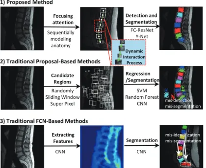
Although numerous methods have been proposed for VB detection and segmentation, they cannot address the above challenges totally. These methods can be attributed into two types: 1. Proposal-based systems usually cause false-positive detection and segmentation results. For this type of system, the VB detection and segmentation task is typically decoupled into the proposing of candidate points (or candidate regions) and the analysis of these candidates. In the first stage, these systems propose points (or regions) with a sliding window [9], sampling-manually [10], super-pixels [11], Shannon entropy[12], or integrating two of the above methods [13]. In the second stage, most of the methods in these systems focus on each candidate region and determine which regions are VBs with a classifier, such as support vector machine (SVM) [10], convolutional neural network (CNN) [9, 13] and random forest classifier (RFC) [11]. These methods only pay attention to the local information, namely the information in candi-date regions, even if these regions are in the background. Thus these methods lead in many

vertebral fracture similar architecture G similar appearance H blurring artifacts I Vertebral body(VB) vertebral fracture F deformed vertebra J joint vertebrae Joint vertebrae K A deformed vertebra B C D E H

Figure 2.1. Challenges in the automatic vertebral body segmentation and detection. Our method is robust to all these challenges. (A) Vertebral Body(VB); (B)(C) Some background tissues present similar architecture or appearance as VBs (or spines), which misleads the detec-tion and segmentadetec-tion; (D)(E) Some adjacent VBs joints together because of some interverte-bral disc lesions, which leads to these joint VBs being detected and segmented as an individual VB; (F)-(K) Complex appearance and various spatial offsets of VBs caused by image artifacts and pathological variations, which imposes great difficulty to accurately detect and segment these VBs.

cases to false-positive detection and segmentation results. While other methods in candidate-level systems, such as [12], uses a graph model to filter out the background and keeps true candidates as VB center points. Such methods do not consider the influence of pathological variations when generating candidate points (or candidate regions). Therefore, the detection and segmentation results are deviated or false-positive. 2. FCN-based systemsusually cau