Repository and Information Exchange
Repository and Information Exchange
Electronic Theses and Dissertations2019
Instance Segmentation and Object Detection in Road Scenes
Instance Segmentation and Object Detection in Road Scenes
using Inverse Perspective Mapping of 3D Point Clouds and 2D
using Inverse Perspective Mapping of 3D Point Clouds and 2D
Images
Images
Chungyup Lee
South Dakota State University
Follow this and additional works at: https://openprairie.sdstate.edu/etd
Part of the Computer Engineering Commons, and the Computer Sciences Commons
Recommended Citation Recommended Citation
Lee, Chungyup, "Instance Segmentation and Object Detection in Road Scenes using Inverse Perspective Mapping of 3D Point Clouds and 2D Images" (2019). Electronic Theses and Dissertations. 3661.
https://openprairie.sdstate.edu/etd/3661
This Thesis - Open Access is brought to you for free and open access by Open PRAIRIE: Open Public Research Access Institutional Repository and Information Exchange. It has been accepted for inclusion in Electronic Theses and Dissertations by an authorized administrator of Open PRAIRIE: Open Public Research Access Institutional Repository and Information Exchange. For more information, please contact [email protected].
INSTANCE SEGMENTATION AND OBJECT DETECTION IN ROAD SCENES USING INVERSE PERSPECTIVE MAPPING OF 3D POINT CLOUDS AND 2D
IMAGES
BY
CHUNGYUP LEE
A thesis submitted in partial fulfillment of the requirements for the Master of Science
Major in Computer Science South Dakota State University
ACKNOWLEDGEMENTS
I am sincerely thankful to Dr. Kwanghee Won, my thesis advisor, for his devotional advice. I am appreciative to have met him. I appreciate his ability to help guide me and provide thoughtful advice. His advice has been helpful and priceless regarding my future in research and directivity.
I appreciate their professional feedback to all of my committee members: Dr. Kwanghee Won, Dr. Yue Zhou, Dr. Sung Shin as well as Dr. Anne-Marie Hoskinson as the graduate faculty representative. Due to their feedback and interest, the quality of my thesis has greatly improved. Aside from that, I cannot forget the time in which I shared with all of the IVS (Intelligent Vision System) lab members.
I would also like to thank my parents. I'd like to thank them for always believing that I am capable of accomplishing another goal within my life. Through them, I was able to safely finish my master’s program.
CONTENTS
LIST OF TABLES ... v
LIST OF FIGURES ... vi
LIST OF EQUATIONS ... vii
ABSTRACT ... viii
INTRODUCTION ... 1
BACKGROUND ... 4
RELATED WORK ... 10
MATERIALS AND METHODS ... 12
CONCLUSION ... 28
LIST OF TABLES
Table 1. the parameters of Mask RCNN [10] ... 26 Table 2. the accuracy of detection between proposed approach and Mask-RCNN [10] .. 27 Table 3. the number of datasets on Mask-RCNN [10] for train, validation, and test ... 27
LIST OF FIGURES
Figure 1. projected images on virtual planes ... 2
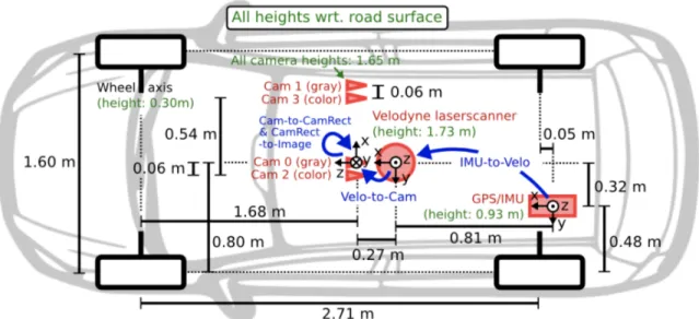
Figure 2. recording platform of KITTI Vision Benchmark Suite [9] ... 4
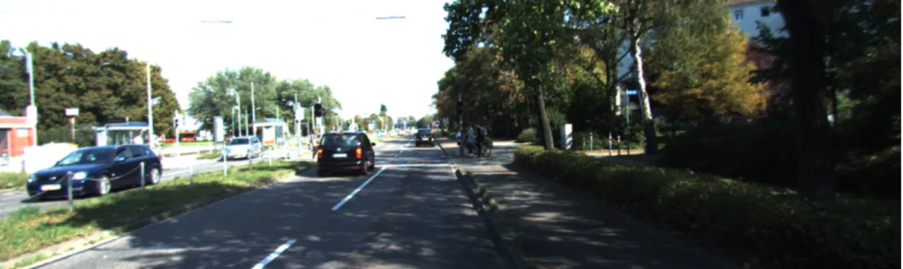
Figure 3. 2D image obtained from a stereo camera ... 5
Figure 4. 3D point cloud obtained from LiDAR sensor ... 5
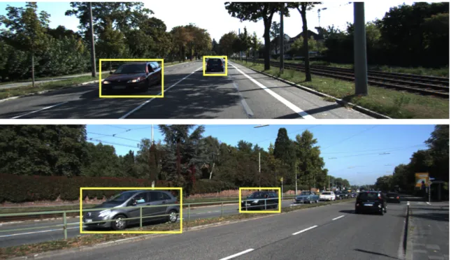
Figure 5. examples of perspective distortion ... 6
Figure 6. typical CNN (Convolutional Neural Network) architecture ... 7
Figure 7. receptive fields through convolution ... 8
Figure 8. object detection and instance segmentation example ... 8
Figure 9. overall process ... 12
Figure 10. a side view of ground plane through plane fitting ... 14
Figure 11. a front view of a virtual image plane and a point cloud ... 16
Figure 12. two intersection lines projected onto an image plane ... 17
Figure 13. a top view of a virtual image plane and a point cloud ... 19
Figure 14. the result from Mask RCNN detection [10] using the pre-processed images . 22 Figure 15. the result from refinement with inverse perspective 3D point map and detection masks ... 22
Figure 16. total loss of Mask RCNN ... 23
Figure 17. loss of bounding box ... 24
Figure 18. loss of class ... 24
Figure 19. loss of RPN (Region Proposal Network) bounding box ... 25
LIST OF EQUATIONS Equation 1 ... 15 Equation 2 ... 15 Equation 3 ... 17 Equation 4 ... 18 Equation 5 ... 19 Equation 6 ... 20
ABSTRACT
INSTANCE SEGMENTATION AND OBJECT DETECTION IN ROAD SCENES USING INVERSE PERSPECTIVE MAPPING OF 3D POINT CLOUDS AND 2D
IMAGES CHUNGYUP LEE
2019
The instance segmentation and object detection are important tasks in smart car applications. Recently, a variety of neural network-based approaches have been proposed. One of the challenges is that there are various scales of objects in a scene, and it requires the neural network to have a large receptive field to deal with the scale variations. In other words, the neural network must have deep architectures which slow down computation. In smart car applications, the accuracy of detection and segmentation of vehicle and pedestrian is hugely critical. Besides, 2D images do not have distance information but enough visual appearance. On the other hand, 3D point clouds have strong evidence of existence of objects. The fusion of 2D images and 3D point clouds can provide more information to seek out objects in a scene.
This paper proposes a series of fronto-parallel virtual planes and inverse perspective mapping of an input image to the planes, to deal with scale variations. I use 3D point clouds obtained from LiDAR sensor and 2D images obtained from stereo cameras on top of a vehicle to estimate the ground area of the scene and to define virtual planes. Certain height from the ground area in 2D images is cropped to focus on objects on flat roads. Then, the point cloud is used to filter out false-alarms among the over-detection results generated by an off-the-shelf deep neural network, Mask RCNN. The experimental result showed that
the proposed approach outperforms Mask RCNN without pre-processing on a benchmark dataset, KITTI dataset [9].
INTRODUCTION
LiDAR sensors and cameras are widely used for smart car applications such as obstacle detection and road detection tasks. Images obtained from a camera provide visual appearance of objects in a scene. However, they do not provide 3D structures nor distance information of the scene which is crucial for many smart car applications. LiDAR sensors, on the other hand, provide 3D point clouds of surrounding environment. The 3D point cloud provides strong evidence of existence of obstacles and road surface. However, typical LiDAR sensors provides sparse (e.g. 16 or 32 vertical sampling points) data. Thus, additional processing is necessary.
Object detection and instance segmentation have been extensively studied. Recently, deep convolutional neural network (CNN)-based approaches showed high-quality detection and segmentation results for flat road scene datasets such as KITTI [9] and CityScape [25] benchmark datasets. On the other hand, instance segmentation on 3D point cloud data has been investigated as well. One of the drawbacks of point-cloud based approaches is that if the object is far from the sensor, the number of 3D points is too small to identify the category of the object. LiDAR and camera fusion can deal with this problem by using both visual appearances obtained from images and strong evidences of presence of obstacles from the point cloud. For these reasons, several LiDAR-camera fusion approaches have proposed [1, 2]. Charles et al. [2] utilized 2D image features obtained by CNN to reduce the search space in 3D view frustum. However, the detection quality is limited by the performance of 2D image segmentation method employed in their architecture.
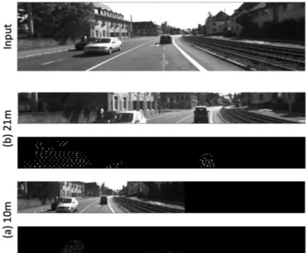
In this paper, I utilize virtual image planes that are fronto-parallel and have the equal heights (of interested objects) from the ground surface and perform inverse-perspective projection of an input image to the virtual image planes [24]. In addition, the corresponding input point cloud is projected to their closest virtual plane. Figure 1 shows two examples of the inverse perspective projection. In Figure 1, The car seen in (b) and the car seen in (a) are represented in the similar scale. The projected 3D points map (a) shows the presence of white car on the left of the image, and (b) shows the presence of black car on the right. This pre-processing can help the segmentation algorithm deal with small objects and the projected point cloud helps removing false alarms.
Top image is an input image from KITTI dataset [9]. (a): the projected input image to a virtual plane at 10 meters away from the focal plane, and projected 3D points to the plane. (b): the projected image and point cloud to the plane at 21 meters.
BACKGROUND 3D Point Cloud and 2D image
3D point clouds are necessary to estimate distance between objects and LiDAR sensor. Velodyne HDL-64E sensor is used to obtain 3D point clouds in KITTI dataset [9] which is an open dataset having road scenes. LiDAR sensor is equipped on top of a vehicle as shown in Figure 2. The sensor emits lights which is reflected from objects to the sensor as it spins 360°. 3D point cloud obtained from the sensor consists of x, y, and z coordinates. Figure 4 shows a point cloud in a scene in 3D space. The black points are 3D points. There are also stereo cameras on top of the vehicle. The cameras can capture 2D images as shown in Figure 3. Each camera has intrinsic and extrinsic parameters which can be expressed as a matrix. The parameters are also provided from KITTI dataset.
Figure 3. 2D image obtained from a stereo camera
Figure 4. 3D point cloud obtained from LiDAR sensor Intrinsic and Extrinsic Parameters
Pinhole cameras have two information which is intrinsic and extrinsic parameters.
Intrinsic parameters consist of focal length (fx, fy) and principal point offset (cx, cy) which
are expressed as a matrix as follows:
𝐾 = $
𝑓& 0 𝑐&
0 𝑓) 𝑐)
0 0 1
Extrinsic parameters have rotation and translation information in a matrix to represent sequences of geometric transformation as follows:
[𝑅|𝑡] = $−𝑠𝑖𝑛𝜃 𝑐𝑜𝑠𝜃 𝑡𝑐𝑜𝑠𝜃 𝑠𝑖𝑛𝜃 𝑡&)
0 0 1
+
Therefore, a camera matrix is expressed as K∙ [𝑅|𝑡].
Perspective Distortion
Perspective distortion is caused by camera position or subject position. The distortion is an fatal problem to detect object in neural networks. Because of the distortion, objects are seen in different size even though they are in the same size. For example, there are two cars in Figure 5. The left car looks approximately 50% bigger than the right car in the same scene because of object position. The two cars are bounded in different sizes.
Convolutional Neural Network
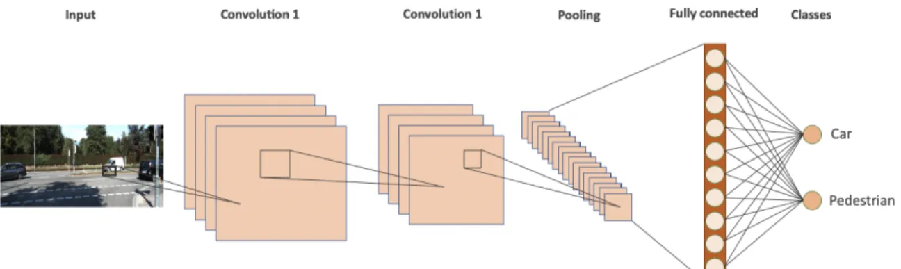
A convolutional neural network is one of deep neural networks to especially analyze visual image. It consists of three parts: input layers, hidden layers, and output layers. There are weights between adjacent layers to extract particular feature maps from the input. Layers of convolutional neural networks are designed depending on certain applications. Figure 6 shows classification for car and pedestrian by feeding 2D image as an input of the network.
Figure 6. typical CNN (Convolutional Neural Network) architecture Receptive Field
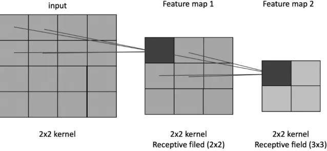
The receptive field is a region of input data as feature maps in convolutional neural networks. For example, there are 2x2 kernel over 4x4 feature map in first convolution and 2x2 kernel over 3x3 feature map in second convolution. First features can be seen 2 by 2 like a black square in the below figure and the second features can be seen 3 by 3 like a yellow square in the below figure 7. The more convolutions over more than 1x1 kernels a neural network has, the larger receptive field it has.
Figure 7. receptive fields through convolution Object Detection and Instance Segmentation
Unlike instance segmentation, object detection provides the classes and also spatial location as bounding box of each class. Instance segmentation provides pixel-wised boundaries of objects. The below figure 8 shows bounding boxes as object detection and masks as instance segmentation. The dotted boxes are bounding boxes to indicate spatial location of the vehicles and the vehicles are masked in each different color.
Figure 8. object detection and instance segmentation example Mask RCNN
There are a variety of RCNNs: Fast RCNN [11], Mask RCNN [10], and YOLO [16]. Especially, Mask RCNN [10] is evolved from Fast RCNN [11] and Faster RCNN
[28] for instance segmentation. This network consists of four kinds of networks: backbone network, region proposal network, classification network, and mask network. the backbone is to extract feature maps and usually weights are used as COCO dataset [26] which is comprised of common objects. region proposal network is to generate region proposals and detect objects on these regions for object detection. Mask network is for masking objects in images for instance segmentation.
RELATED WORK
Point Cloud and 2D Image Fusion: Yang et al. [21] proposed that stereo image point cloud and LiDAR Point cloud fusion to make up for advantages and disadvantages of each point cloud because LiDAR point cloud is accurate and stereo image point cloud is dense. The approach provides a consistent and detailed 3D reconstruction in street environment. Real-time 3D perception is so important lately that Will et al. [23] proposed a probabilistic method to provide an accurate depth map by estimating disparity map with LiDAR and stereo sensor.
There is a deep learning-based road detection method proposed by Luca et al. [22]. The approach used both image and LiDAR data as input of the deep convolutional neural network. Ming et al. [1] proposes 3D object detection in continuous convolutions by fusing LiDAR and image feature maps which are seen at different levels of resolution. Qi et al. proposed a 3D object detection method especially for 3D localization of the detected object in large-scale scenes [2]. They utilized 2D object detector to constrain the object detection in 3D point cloud.
Deep Neural Networks for 3D Point Clouds and Images 3D data and 2D image are considered as the most typical inputs in neural networks for computer vision tasks [3, 4, 8, 10, 11, 14, 16]. The 3D point cloud has been used even though it has alignment problem [5]. The PointNet proposed by Charles et al. [3] uses raw point clouds, while VoxelNet proposed by Yin et al. [14] uses a voxel representation for 3D point clouds. However, it is not easy to learn features on point clouds due to the sparsity and the additional z-axis make the process slow compared to the case of 2D images. Recently, Fast R-CNN [11] and Mask R-CNN [10] are proposed and they are the pioneers of efficient instance segmentation and
object detection on 2D images. They utilize Resnet [6] or FPN [7] to extract multi-scale features [13, 15].
MATERIALS AND METHODS
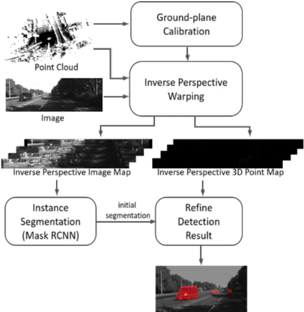
The pre-processing has two parts: ground-plane calibration and inverse perspective warping. In these parts, virtual image plane and inverse perspective 3D point map are generated. For the instance segmentation, Mask RCNN [10] is used. Afterwards, detections are refined to discard false alarms. Each box bellow will be explained in detail in this section.
Image Projection on Virtual Planes
The proposed pre-processing method consists of two steps: calibration of the ground-plane and vertical virtual planes and inverse perspective projection of input image and point clouds. First, the calibration carries out plane fitting to properly locate virtual planes of same height at predefined distances from the focal plane. (Ground-Plane Calibration section and Generating Virtual Image Plane section) Then, I project the 3D point cloud and the input image to the virtual planes to create inverse perspective 3D point maps and image strips that have the same heights. The point map is useful to decide if vehicles exist near the plane and the warped image strips will be stacked and fed into the Mask RCNN for instance segmentation. (Inverse Perspective 3D Point Map section and Image Warping section) In this research, I use a subset of KITTI dataset [9] which consists of point clouds, gray/RGB images, and calibration information. Figure 9 shows the overall steps of the proposed approach and Figure 1 shows sample outputs of the pre-processing step.
Ground-Plane Calibration
Plane fitting is the first process of the pre-processing using a point cloud for ground
estimation [20]. The point cloud is a collection of 3D points represented by a set of {Pi | i
= 1, ..., n}, where each Pi represents a vector of (x, y, z) coordinate. Given a point cloud, RANSAC is used to select randomly a subset of the 3D points. Besides, PCA [12] is used as a technique to stress variations and derive strong patterns in a dataset. I can acquire PC1, PC2, and PC3 which of each represents strength of variations. PC3 is orthogonal to both PC1 and PC2, which means a normal vector of the ground plane.
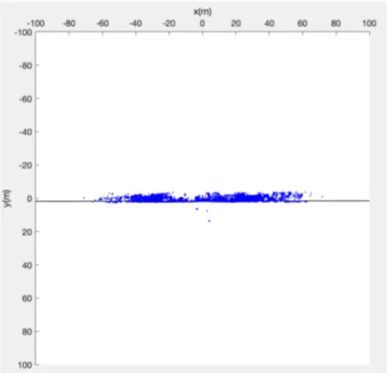
Figure 10. a side view of ground plane through plane fitting
Coordinate (x, y) represents distance meter. The blue points are 3D points in a scene and the black line is a side view of the ground plane. Figure 10 shows a side view of a point cloud and a ground plane. The x-axis represents width and y-axis represents height. Both values mean distance meter. The blue points are 3D points in an urban scene. The black line is a side view of the ground plane obtained from a PC3 vector. Intuitively, almost all points are on the ground plane.
Generating Virtual Image Plane
I can move forward an image plane as inputs in specific distances in the 3D space in order to gain constant scale image which is called a virtual image plane. First, rays from camera origin to image corner are found. Here, there is an intrinsic matrix of a camera from KITTI dataset [9]. I can easily derive the ray vectors:
8 → := K -1P R = ; 8 → <,→8>,→8?,→8@A (1)
where K is an 3x3 intrinsic matrix and P is a corner point (x, y, 1) of an image plane in 3D
space. R is a set of 4 rays, where each Ri is a ray vector from a camera origin to image
plane corners. Virtual image planes in Figure 11 can be generated is as follows: R' = Pd(R)
Pd(R) = (𝑉D⃗ ∙ R) × R
𝑉D⃗ = T × d
(2)
where R is a set of ray vectors and R' is a new set of ray vectors which have a specific
distance as 𝑑 toward corners of an image plane. 𝑉0 is a ray vector with specific distance
from camera origin toward a center of the image plane and T is a translation matrix. The virtual image planes generated by (2) are warped to keep the object size constant as well as they are used for feature extraction in many different kinds of distances.
Figure 11. a front view of a virtual image plane and a point cloud
The output from the above section forms [PC1, PC2, PC3], where PC3 is a normal vector of the ground plane. I have two normal vectors. One is PC3 and another one is a normal vector of virtual image plane which is called Vnorm. I can find intersection lines between the ground plane and virtual image planes generated from (2) by a vector of PC3 × Vnorm. The new vector from cross product of PC3 and Vnorm is used to discard redundant parts in an image plane. The bottom part of a vehicle is unnecessary for seeking out vehicles in a neural network. I discard the top part of vehicles, as well. The blue line in the top is obtained from the PC3 at specific height. Finally, the two intersection lines are projected onto the image plane as seen in Figure 11.
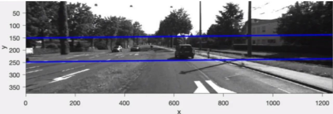
Figure 12. two intersection lines projected onto an image plane
Two blue lines represent the top and bottom of a virtual image plane. By cutting off the outside of the two blue lines, Features between the two blue lines are concentrated in Mask RCNN [10] without extracting redundant features and region proposal.
Inverse Perspective 3D Point Map
Inverse perspective 3D point maps are produced to cue vehicle existence to the detection refinement after instance segmentation [10]. The virtual image plane as output from the above section is used to select candidates of 3D points. All of x and y coordinates of candidate points must be inside of a given virtual image plane, which can be obtained by simple calculation as follows:
𝑓(𝑃) = J1, 𝐴𝑟𝑒𝑎 = ∎𝐴𝐵𝐶𝐷0, 𝑜𝑡ℎ𝑒𝑟𝑤𝑖𝑠𝑒
Area = ∆𝑃𝐴𝐵 + ∆𝑃𝐴𝐶 + ∆𝑃𝐵𝐷 + ∆𝑃𝐶𝐷
(3)
where the Area function is to add all of four triangle areas with regard to the point P. Each
point of ABCD is corner points of the virtual image plane. The function 𝑓(𝑃) is to decide
the area of the virtual image plane, it means there is a point inside the virtual image plane.
After (3), the point must be in a given distance θ along z-axis. In my case, I used 1m.
Figure 13 shows candidate points as red points inside of the black line as the virtual image plane.
The selected candidate points are projected onto the image plane. I can produce inverse perspective 3D point maps as the 3rd image and 5th image in Figure 1. The projected points have distance values and others are black. I can define the projection matrix from [9]:
P = 𝑃W× 𝑅W× [𝑅|𝑇] (4)
where 𝑃 is a 3×4 projection matrix after rectification, 𝑅 is a 4×4 rectifying rotation, R is a
4×3 rotation matrix of camera, and T is a 4×1 translation matrix of camera. The projected points are used to improve vehicle detection.
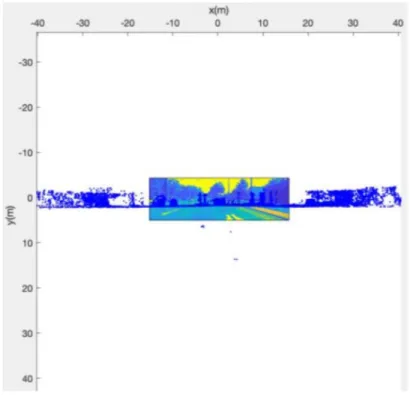
Figure 13. a top view of a virtual image plane and a point cloud
The blue points are input 3D points and the red points are the points that are within one meter distance from the virtual image plane (black line).
Image Warping
The output from the above step is a cropped image after discarding unnecessary parts. In order to warp the both images, I need the homography matrix [19] which is a matrix to represent sequences of geometric transformations as affine transformations.
I' = I(H(x, y)) (5)
where H is a homography matrix and I is an input image. x and y are coordinates of an image. I' is a warped image in (5) and it is taken as input of the network.
Before warping, we must calculate new image scale with respect to fixed height. We can define the new width as follows:
W' = YZ× W (6)
where W’ is a new width, H is a height in fixed size which is 73 pixels in our case, W is the width of an original image, and h is a distance between the two intersection lines. I used 14 images with different distances and fixed height which are in 1024x1024 as an input of Mask RCNN. Inputs of the network must be able to be divided by 64 pixels because the network uses 6 layers of pyramid network and two feature maps are added after up-sampling and down-up-sampling.
Instance Segmentation and Refinement
We use the off-the-shelf neural network architecture [10] for instance segmentation. The output from the pre-processing step is fed as input in the network. The image size 1024×1024. Each vehicle is detected and masked in the network. The masks are used to improve an accuracy of vehicle detections in optimal distances.
The masks are covered on the inverse perspective 3D point maps which have distance values between virtual image plane and nearby 3D points so that I can know the approximate distance of objects. For refinement, the masks are filtered out first by checking if there are points inside the masks. The refined masks are warped back again into the original image using an inverse of the homography matrix used in the previous step (Sec. Inverse Perspective 3D Point Map) [19]. The masks which have the same attribution of vehicles are densely overlapped on the original input image. The overlapped masks are filtered by the distance values of inverse perspective 3D point map. The single mask
remains for each vehicle, which indicate the actual distance (the distance of the closest virtual plane).
RESULT AND ANALYSIS
Figure 14. the result from Mask RCNN detection [10] using the pre-processed images
Figure 15. the result from refinement with inverse perspective 3D point map and detection masks
Figure 14 and Figure 15 show the experimental results of the proposed approach. A subset of KITTI dataset is used for the experiment. The provided calibration information
is used to align LiDAR data and image data. The dataset is labeled by using Via Annotation Software [18] and the labeled information as polygonal shape data is saved in JSON format [29]. I used Tensorflow framework [27] which provides all of components to build up neural networks for instance segmentation and object detection of Mask RCNN [10]. The experiment has conducted on an Ubuntu machine with two NVIDIA GeForce GTX 1080 Ti and Intel(R) Core (TM) i7-7800X CPU @ 3.50GHz. Figures below show loss is gradually decreasing which means all of networks in Mask RCNN is convergent for the dataset. Figure 16 is total loss of whole networks in Mask RCNN.
Figure 17. loss of bounding box
Figure 19. loss of RPN (Region Proposal Network) bounding box
Table 1 show the number of parameters. it depends on neural network architecture and input size. I have 1024x1024 input size and Mask RCNN architecture. The total number of parameters is 63,733,406. I have 21,069,086 trainable parameters because I used the backbone as ResNet101 with pre-trained weight which is not necessary to be trained again.
Table 1. the parameters of Mask RCNN [10]
Name # of parameters Trainable parameters 21,069,086 Non-trainable parameter Total parameter 42,664,320 63,733,406
The network has ResNet101 [6] as a backbone to extract feature maps. I used pre-trained weights obtained from COCO dataset [26] which consists of common objects. I loaded the pre-trained weight values onto the backbone network. Other networks (Region proposal network, classification network, and mask network) were retrained with 502 training data which include 2574 vehicles for 100 epochs, and 83 images which include 419 vehicles were used for validation. The learning rate is 0.001, the learning momentum is 0.9, and the batch size is 2. The accuracy is measured for 100 test images which include 520 vehicles for both the proposed and the Mask RCNN without LiDAR data. The Table 2 shows the proposed approach outperforms the image-only approach. Figure 13 shows the detection results for both approaches. The vehicles that are not detected with the image-only approach are successfully detection with the proposed approach.
Figure 15 shows the refined distances of detection vehicles using the inverse perspective map of 3D points along with distances. After the refinement, I can determine the distance of each vehicle in the scene based on the approximate distance of the corresponding virtual plane.
Table 2. the accuracy of detection between proposed approach and Mask-RCNN [10]
Input scenes vehicles detections Detection
Accuracy
Proposed Approach 100 520 483 93.0 %
Mask R-CNN 100 520 412 81.0 %
Table 3. the number of datasets on Mask-RCNN [10] for train, validation, and test
Dataset Scenes Vehicles
Training 502 2574
Validation 83 419
CONCLUSION
This paper proposed pre-processing and post-processing methods for the Mask RCNN to improve the detection performance on road scene images. I assume vehicles are on flat road. The images are projected to a series of virtual planes to have the same scale when there is any object in it. The projected LiDAR data are used to filter out the false-alarms over-detected at neighboring virtual planes. The experimental results show that the proposed approach improves an accuracy of vehicle detection on a subset of KITTI dataset [9].
In the future, I will investigate to utilize LiDAR data for improving the quality of region proposals in the Mask RCNN architecture [10]. Mask RCNN computation is dependent on the number of region proposals. LiDAR data are used for a strong evidence of existence of objects, which is able to filter out redundant region proposals by providing additional information into the region proposal network. For improving computation time, I will reduce layers of the ResNet50/101 architecture [6] as a backbone which is used to extract feature maps in Mask RCNN. Scales of objects of the pre-processed dataset are invariant so that even small layers of a backbone would work for extracting enough feature maps.
LITERATURE CITED
1. Ming Liang, Bin Yang, Shenlong Wang, and Raquel Urtasun. Deep Continuous
Fusion for Multi-Sensor 3D Object Detection. The European Conference on Computer Vision (ECCV), 2018, pp. 641-656.
2. Charles R. Qi, Wei Liu, Chenxia Wu, Hao Su, Leonidas J. Guibas: Frustum
PointNets for 3D Object Detection from RGB-D Data. arXiv:1711.08488. 2018.
3. Charles R. Qi, Hao Su, Kaichun Mo, Leonidas J. Guibas: PointNet. Deep Learning
on Point Sets for 3D Classification and Segmentation. 10 Apr 2017.
4. Jonathan Long, Evan Shelhamer, Trevor Darrell. Fully convolutional networks for
semantic segmentation. 7-12 June 2015.
5. R. B. Rusu, N. Blodow, Z. C. Marton, and M. Beetz. Aligning point cloud views
using persistent feature histograms. In 2008 IEEE/RSJ International Conference on Intelligent Robots and Systems, pages 3384–3391. IEEE, 2008.
6. Kaiming He, Xiangyu Zhang, Shaoqing Ren, Jian Sun. Deep Residual Learning for
Image Recognition. 10 Dec 2015.
7. Tsung-Yi Lin, Piotr Dollár, Ross Girshick, Kaiming He, Bharath Hariharan, Serge
Belongie: Feature Pyramid Networks for Object Detection. 19 Apr 2017.
8. Gusi Te, Wei Hu, Zongming Guo, Amin Zheng. RGCNN: Regularized Graph CNN
for Point Cloud Segmentation. 8 Jun 2018.
9. Andreas Geiger, Philip Lenz, Christoph Stiller and Raquel Urtasun. Vision meets
Robotics: The KITTI Dataset. 2013.
10. Kaiming He, Georgia Gkioxari, Piotr Dollár, Ross Girshick. Mask R-CNN. 24 Jan
11. Ross Girshick: Fast R-CNN. 27 Sep 2015.
12. Jonathon Shlens. A Tutorial on Principal Component Analysis. December 10, 2005.
13. Vincent Dumoulin, Francesco Visin. A guide to convolution arithmetic for deep
learning. 11 Jan 2018.
14. Yin Zhou, Oncel Tuzel. VoxelNet: End-to-End Learning for Point Cloud Based 3D
Object Detection. 17 Nov 2017.
15. Karen Simonyan, Andrew Zisserman. Very Deep Convolutional Networks for
Large-Scale Image Recognition. 10 Apr 2015.
16. Joseph Redmon, Santosh Divvala, Ross Girshick, Ali Farhadi. You Only Look
Once: Unified, Real-Time Object Detection. 9 May 2016.
17. Kaiming He, Xiangyu Zhang, Shaoqing Ren, Jian Sun. Spatial Pyramid Pooling in
Deep Convolutional Networks for Visual Recognition. 23 Apr 2015.
18. Abhishek Dutta, Andrew Zisserman. The VIA Annotation Software for Images,
Audio and Video. 31 May 2019.
19. Richard Hartley, Andrew Zisserman. Multiple View Geometry in Computer Vision.
2003.
20. Nina M. Varney, Vijayan K. Asari. Volume Component Analysis for Classification
of LiDAR Data. 2015.
21. Yuan Yang, Zoltan Koppanyi, Charles K Toth. Stereo Image Point Cloud and
LiDAR Point Ccloud Fusion for The 3D Street Mapping. 2017.
22. Luca Caltagirone, Mauro Bellone, Lennart Svensson, Mattias Wahde. LIDAR-
Camera Fusion for Road Detection Using Fully Convolutional Neural Networks. 21 Sep 2018.
23. Will Maddern, Paul Newman. Real-time probabilistic fusion of sparse 3D LIDAR and dense stereo. October 2016.
24. M. Park, and S.K. Jung, “GPU-Based Real-Time Pedestrian Detection and Tracking
Using Equi-Height Mosaicking Image”, International Conference on Neural Information Processing, 2013.
25. Marius Cordts, Mohamed Omran, Sebastian Ramos, Timo Rehfeld, Markus
Enzweiler, Rodrigo Benenson, Uwe Franke, Stefan Roth, Bernt Schiele.The Cityscapes Dataset for Semantic Urban Scene Understanding. 6 Apr 2016.
26. Tsung-Yi Lin, Michael Maire, Serge Belongie, Lubomir Bourdev, Ross Girshick, James Hays, Pietro Perona, Deva Ramanan, C. Lawrence Zitnick, Piotr Dollár. Microsoft COCO: Common Objects in Context. arXiv:1405.0312, 1 May 2014. 27. Martín Abadi, Ashish Agarwal, Paul Barham, Eugene Brevdo, Zhifeng Chen, Craig
Citro, Greg S. Corrado, Andy Davis, Jeffrey Dean, Matthieu Devin, Sanjay Ghemawat, Ian Goodfellow, Andrew Harp, Geoffrey Irving, Michael Isard, Rafal Jozefowicz, Yangqing Jia, Lukasz Kaiser, Manjunath Kudlur, Josh Levenberg, Dan Mané, Mike Schuster, Rajat Monga, Sherry Moore, Derek Murray, Chris Olah, Jonathon Shlens, Benoit Steiner, Ilya Sutskever, Kunal Talwar, Paul Tucker, Vincent Vanhoucke, Vijay Vasudevan, Fernanda Viégas, Oriol Vinyals, Pete Warden, Martin Wattenberg, Martin Wicke, Yuan Yu, and Xiaoqiang Zheng. TensorFlow: Large-scale machine learning on heterogeneous systems, 2015, ISBN 978-1-931971-33-1.
28. Shaoqing Ren, Kaiming He, Ross Girshick, Jian Sun. Faster R-CNN: Towards Real-Time Object Detection with Region Proposal Networks. 4 Jun 2015,
arXiv:1506.01497
29. Geoff Langdale, Daniel Lemire. Parsing Gigabytes of JSON per Second. 22 Feb 2019, arXiv:1902.08318