Predictive Analytics for Complex IoT Data Streams
Adnan Akbar, Abdullah Khan, Francois Carrez, and Klaus Moessner
Abstract—The requirements of analyzing heterogeneous data streams and detecting complex patterns in near real-time have raised the prospect of Complex Event Processing (CEP) for many internet of things (IoT) applications. Although CEP provides a scalable and distributed solution for analyzing complex data streams on the fly, it is designed for reactive applications as CEP acts on near real-time data and does not exploit historical data. In this regard, we propose a proactive architecture which exploits historical data using machine learning (ML) for prediction in conjunction with CEP. We propose an adaptive prediction algorithm called Adaptive Moving Window Regression (AMWR) for dynamic IoT data and evaluated it using a real-world use case with an accuracy of over 96%. It can perform accurate predictions in near real-time due to reduced complexity and can work along CEP in our architecture. We implemented our proposed architecture using open source components which are optimized for big data applications and validated it on a use-case from Intelligent Transportation Systems (ITS). Our proposed architecture is reliable and can be used across different fields in order to predict complex events.
Index Terms—Complex event processing, data streams, inter-net of things, machine learning, predictive analytics, proactive applications, regression, time series prediction
I. INTRODUCTION
Internet of things (IoT) has significantly increased the num-ber of devices connected to the Internet ranging from sensors and smart phones to increasingly soft aspects such as crowd sensing or users as sensors. The availability of data generated by these diverse devices has opened new opportunities for innovative applications across different fields; supply chain management systems [1], Intelligent Transportation Systems (ITS) [2] and smart buildings [3] are few of them.
Most of IoT applications such as traffic management system or supply chain logistics of big super markets involve large data sets which have to be analyzed in near real-time in order to make decisions. Data from different sensors in IoT is generated in the form of real-time events which often form complex patterns; where each complex pattern represents a unique event. These unique events must be interpreted with minimal time latency in order to apply them for decision mak-ing in the context of current situation. The need for processmak-ing, analyzing and inferring from these complex patterns in near real-time forms the basis of a research area called Complex Event Processing (CEP) [4]. It includes processing, analyzing, and correlating event streams from different data sources to infer more complex events in near real-time. The inherent distributed nature of CEP [5] makes it ideal candidate for many IoT applications as evident by examples found in literature A. Akbar, F. Carrez and K. Moessner are with the Institute for Communi-cation Systems, University of Surrey, UK (email: [email protected]; [email protected]; [email protected])
A. Khan is with department of Information Engineering, University of Pisa, Italy (email: [email protected]
for instance analyzing real-time traffic data [6] or providing automatic managing systems for smart buildings [7].
CEP provides solutions to deal with data streams in near real-time but it lacks the predictive power provided by many machine learning (ML) and statistical data analysis methods. Most of the CEP applications found in the literature are intended to provide reactive solutions by correlating data streams using predefined rules as the events happen and does not exploit historical data due to its limited memory. However, in many applications, prediction of a forthcoming event is more useful than detecting it after it has already occurred. For example, it will be more useful to predict traffic congestion as compared to detecting it, so that traffic administrators can take preventive measures to avoid it. The advantages of predicting an event are more obvious if we imagine the gain of predicting natural disasters and epidemic diseases.
On the other hand there are several methods found in literature based on ML and statistics which have the ability to provide innovative and predictive solutions in different domains, for example predicting passengers travel time for ITS [8] and energy demand for buildings [9] are two of the many examples found in literature. However, they are not suitable for analyzing and correlating different data streams in near real-time as they require historical data to train the models. ML methods exploit historical data and applies diverse approaches such as probability, statistics and linear algebra to train the models in order to make predictions about the future. They have the potential to provide the basis for proactive solutions for IoT applications but they lack the power of scalability and processing multiple data streams in real-time which is provided by CEP.
A. Related Work
In literature, CEP and ML have been explored extensively as separate research fields and were mostly targeted for different types of applications. CEP has been designed for processing and correlating high speed data on the fly without storing it [5]. Whereas ML methods are targeted for applications which are based on the historical data for extraction of knowledge [10].
In recent years, the diverse requirements for processing data in IoT led to the increase of hybrid approaches where predictive analytics (PA) methods based on ML and statistics are combined with CEP in order to provide proactive solutions. Initially, it was proposed in [11], where authors presented a conceptual framework for combining PA with CEP to get more value from the data. The approach of combining both methods lead to encouraging results; however, they did not support their idea with any practical application. Another example is given in [12] where authors used probabilistic
event processing network to detect complex events and then used these complex events to train multi-layered Bayesian model to predict future events. Their proposed prediction model employs expectation maximization (EM) algorithm [13]. EM being an iterative optimization algorithm has high computational cost. Its complexity increases exponentially as the training dataset increases, therefore making it unsuitable to large scale IoT applications. They demonstrated their solution on the simulated traffic data with the assumption of availability of statistical data of vehicles which is unlikely to be available in a real-world use-case.
In [14], authors provide a basic framework for combining time series prediction with CEP to monitor food and phar-maceutical products in order to ensure their quality during the complete cycle of supply chain. The authors highlighted the open issues related to prediction component such as model selection and model update as new data arrives but they did not address these issues and left it for their future work. Another example of using time series prediction of data for CEP in order to provide predictive IoT solutions is mentioned in [15], where authors implemented neural network for prediction. They demonstrated their approach on the traffic data and used 60 days of data to train the neural network. Once trained, model parameters are static which is a major drawback. The statistics and behavior of underlying data may change over time due to concept drift [16] which can effect the accuracy and performance of the neural network. The model is unable to update and adapt to changes. In case of erroneous readings, errors will propagate and potentially will keep on increasing eventually effecting the reliability of the system.
In literature, prediction using conventional machine learning methods have also been deployed for real-time applications. One such work is mentioned in [17], where authors demon-strated the use of traditional machine learning algorithms for predicting the trajectory of sea vessels in real-time. They implemented their system using Massive Online Learning (MOA) framework [18] which is an open source tool for scalable data stream mining. They proposed a service based system where models are trained using large historical data and saved in a service container which can be called by queries to get the prediction result. Such service based methods are not compatible with event driven systems like CEP. In service based systems, data is pulled with every request in contrast to CEP systems where data is pushed continuously.
B. Motivation
CEP enables to correlate data coming from heterogeneous sources and extract high-level knowledge. Most CEP systems have SQL-like query language which enables to perform tasks like filtering, aggregation, joint and sliding window operations on different data streams and combine it with the help of simple rules. In contrast to batch processing techniques which store the data and later run queries on it, CEP instead stores queries and runs data through these queries. The inbuilt capa-bility of CEP to handle multiple seemingly unrelated events and correlate them to infer complex events provides CEP an edge on ML methods for many IoT applications. However, the
notion of many IoT applications have changed from reactive to proactive in recent times leading to many research efforts towards hybrid solutions based on ML and CEP.
Although there is growing interest in the research com-munity to combine CEP and ML for predicting complex events, most of the research conducted in this direction is theoretical and lacks implementation details or real-world use-case examples. To the best of authors knowledge, no work in literature has addressed the different challenges and open re-search issues for the efficient implementation of ML prediction with CEP. The complexity of underlying ML algorithms play an important role as more complex algorithms are not suitable for real-time prediction and are unable to cope with the fast and dynamic IoT data streams. Although, streaming regression algorithms (e.g. Spark Streaming [19]) based on micro batch analysis [20] can provide faster solution but these algorithms do it at the expense of less accuracy. In our earlier work [21], we proposed a solution highlighting these drawbacks and presented initial results. In this paper, we improve our initial approach, extend our experimental evaluation and implement the overall architecture using open source components which are optimized for large scale IoT data.
C. Contributions
Following contributions are made in this paper.
• We propose and implement a generic architecture based on open source components for combining ML with CEP in order to predict complex events for proactive IoT applications.
• We propose an adaptive prediction algorithm called Adaptive Moving Window Regression (AMWR) for dynamic IoT data streams and implemented it on a real-world use-case of ITS achieving accuracy up to 96%. In our work, we proposed a novel method for finding optimum size for training window by exploiting spectral components of time series data.
• We model the error introduced by our prediction algorithm using a parametric distribution and derive expressions for the overall error of the system, as the error propagates through the CEP.
D. Organization
The remainder of the paper is organized as follows. Section II explains our proposed architecture along with the descrip-tion of different components involved for the implementadescrip-tion of our solution. We have demonstrated the feasibility of our proposed solution by implementing a prototype and evaluating the results on a real-world use-case scenario in Section III. Finally we draw conclusion and highlight our future work in section IV.
II. PROPOSEDARCHITECTURE
The proposed architecture illustrating our approach is shown in the Figure 1. One of the priority of our research is to propose a practically implementable solution and therefore, we have opted for scalable open source components. There are several
Historical Data Adaptive Moving Window Regression (AMWR) Predicted data Kafka Event Collector Complex Event Engine Event Producer
Kafka Esper CEP Engine
Data Source 2 Node-RED
Data Source 1
Data Source 3
Real-time data
Python scikit-learn
Fig. 1. Proposed Architecture and Block Diagram
issues which needed to be considered when choosing different components for the proposed architecture such as scalability and reliability of the system, integration of ML component with CEP, exchange of data across different components in near real-time, a common data format across all components in the architecture, are few of them.
In our architecture, Node-RED [22] provides the front end where data from different sources such as MQTT data feeds or a RESTful api are accessed; and after performing pre-processing tasks such as filtering redundant data and convert-ing to required data format; it is published under a specific topic on the Kafka message broker. More details about the Kafka and Node-RED can be found in the next section. The AMWR block represents the ML component, it accesses the real-time data from the Kafka topic and publishes back the predicted data under different topic on Kafka in the form of an event tuple. The implementation was done in python using Scikit-learn module [23]. The event collector module of CEP is listening to events and as soon as new events are available, it collects them, performs pattern matching using CEP engine and produces the complex events.
More details about the proposed prediction algorithm and different components involved in our architecture are described below.
A. Adaptive Moving Window Regression (AMWR)
We propose and develop an adaptive prediction algorithm called Adaptive Moving Window Regression (AMWR) for dynamic IoT data. In general, prediction models are trained using large historical data and once the model is trained it is not updated due to limitations posed by large training time. Such models are not optimized to perform under phenomenon such as concept drift [16].
The context of the application may change resulting in the degradation of performance for prediction model. For such scenarios, we propose a prediction model which utilizes moving window of data for training the model; and Once
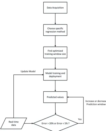
new data arrives, it calculates an error and retrains the model accordingly. We proposed to find the optimum size for training window by exploiting spectral components of time series data using Lomb Scargle method [24]. Our proposed approach is adaptive in nature as it tracks down errors and prevents it from propagating by retraining the model periodically. The size of the prediction window or forecast horizon is also adaptive and is derived by the performance of the model in order to ensure a certain reliability in the prediction. The flowchart of the overall approach is shown in the Figure 2. There are three main steps involved in the implementation of AMWR as described below:
1) Selection of regression algorithm;
2) Finding optimum training window size;
3) Size of the prediction horizon.
1) Selection of Regression algorithm: There are several algorithms available for time series regression (prediction) ranging from statistical to pure ML domain. Traditionally, sta-tistical methods like auto regressive moving average (ARMA) and auto regressive integrated moving average (ARIMA) [25] were used for time series regression. However, recently the trend is shifted towards more sophisticated ML models such as different variants of support vector regression (SVR) and artificial neural networks (ANN) because of their robustness and ability to provide more accurate solutions. We have implemented our approach using SVR due to its ability to model non-linear data using kernel functions. SVR is an extension of SVM which is widely used for regression analysis [26]. The main idea is the same as in SVM, it maps the training data into higher feature space using kernel functions and find the optimum function which fits the training data using hyper-plane in higher dimension. Methods based on SVR often provide more accurate models as their counterpart regression algorithms at the expense of additional complexity. However, as in our algorithm we propose to use a small training window, the added complexity is almost negligible for such small datasets. We compared the performance of several variants of SVR and finally SVR with radial basis function
Data Acquisition Data Acquisition Choose specific regression method Choose specific regression method Find optimized training window size
Find optimized training window size
Model training and deployment Model training and
deployment Error > 20% or Error < 5% ? Error > 20% or Error < 5% ? Real-time data Real-time data Predicted values Predicted values Increase or decrease Prediction window Update Model Yes
Fig. 2. Flowchart for Adaptive Moving Window Regression
(RBF) kernel was chosen as underlying regression algorithm. 2) Optimum Training Window Size: The choice of the optimum training window size for ML models is an open research issue. In general, the accuracy of prediction model increases as the size of training data increases which reflects to have large historical data for training prediction models so that it covers all possible patterns spanning time series. Although this approach generates generic and accurate model for prediction in most cases, there is one major drawback associated with it which was mentioned earlier as well: If the behavior or statistics of the underlying data changes, trained model is unable to track the changes and result into erroneous readings and the error will start accumulating in future predictions.
In contrast to this approach, researchers have proposed to use the moving window for training the ML model in which most recent data is fed to the models. The size of the optimum window is a challenging task with no generic solution. A large window size can have more accurate results but it increases the complexity of the model making it unsuitable for real-time applications whereas a small window size can result into an increased error and hence effecting the reliability of the system.
In order to overcome this issue, we propose a novel and generic method based on time series analysis (Lomb Scargle method) to find the optimum window size and validated our results using real-world data. In our method, we exploited the inherit periodic nature of most of the real world time series data. Consider a simple example of a temperature data
generated by a sensor deployed in Rio de Janeiro, Brazil [27] as shown in the Figure 3; although the pattern formed by the temperature data is very irregular, a repeating pattern in the temperature readings can be observed after every twenty four hours. In our approach, we exploit the fact that if the training window used is equal to the inherent periodicity of the data, it will learn all the local patterns and would be able to predict more accurately. It should be noted that our approach does not assume the underlying data as periodic but instead looks for the highest periodic component.
Fig. 3. Temperature Data [27]
A Fast Fourier Transform (FFT) algorithm is the most commonly used method for finding periodicity by searching for the sharp peaks in the periodogram calculated by Fourier transform of the time series. FFT requires the time series to be evenly spaced which is not always possible for most of the IoT data. Missing values is a common phenomenon in IoT and the inability of FFT to deal with it makes it unsuitable for our system. For such systems, another method called least-squares spectral analysis (LSSA) or more commonly known as Lomb Scargle can be used to find the highest periodic component in a time series data. Lomb first proposed the method while studying variable stars in astronomy [24] and is defined by following equations: PX(f) = 1 2σ2 ( N P n=1 (x(tn)−x)cos(2πf(tn−τ)) 2 N P n=1 cos2(2πf(t n−τ)) + PN n=1 (x(tn)−x)sin(2πf(tn−τ)) 2 N P n=1 sin2(2πf(t n−τ)) ) (1)
wherexandσ2 are the mean and variance of data and the
value ofτ is defined as tan(4πf τ) = N P n=1 sin(4πf tn) N P n=1 cos(4πf tn) (2)
In our architecture, we have used Lomb Scargle method to find optimum window size for training ML models.
3) Adaptive Prediction Window: In our work, we propose to have an adaptive size for prediction window or more commonly known as prediction horizon in order to ensure a certain level of accuracy. The intuition behind it is to
increase the size of prediction window if the accuracy of model is high and decrease it if the performance of the prediction model decreases. The performance of the model is evaluated by comparing the predicted data with actual data when it arrives. Algorithm 1 shows our approach for adaptive prediction window.
Algorithm 1 Adaptive Prediction Window Size 1: function PREDICTIONWINDOW(yact, ypred)
2: M AP E=mean(abs((yact−ypred)/yact)∗100) 3: if M AP E >20% then
4: P redictionW indow=P redictionW indow−1
5: else ifM AP E <5%then
6: P redictionW indow=P redictionW indow+1
7: else
8: P redictionW indow=P redictionW indow
9: end if
10: returnP redictionW indow 11: end function
B. Other Components
A brief introduction of components used in our architecture is given below.
1) Node-RED: Node-RED serves as the front-end interface for our architecture. IoT has provided the researchers with a global view enabling access to truly heterogeneous data sources for the very first time. These data sources can be RESTful web service, MQTT data feed or any other external data source. Data format is not limited to any specific format in IoT. XML and JSON are two most commonly used formats which are used extensively for transmitting IoT data. Also, different data feeds from different sources may contain data which might be redundant for a specific application and needs to be filtered out. Node-Red provides all of these functionali-ties with a fast prototyping capacity to develop rapid wrappers for heterogeneous data sources.
Node-RED is an open source visual tool which is used extensively for wiring the Internet of Things. It provides APIs for connecting different components, and with the help of user provided Java code, it can be used to filter the data change the format as well. It is designed to make the process of integration of different components and data sources in IoT easier.
2) Apache Kafka: We have used Apache Kafka as the message broker for real-time generated events. It is also an open source tool for real-time publishing and subscribing of messages or data. It provides a scalable architecture for high throughput data feeds with very low latency. It was developed by LinkedIn and was open sourced later in 2011. Like other publish-subscribe messaging systems, Kafka maintains feeds of messages in topics. Producers write data to topics and consumers read from topics. Since Kafka is a distributed system, topics are partitioned and replicated across multiple nodes. A single topic can have one or more consumers. Messages are simply byte arrays and the developers can use them to store any object in any format with String, JSON,
and Avro being the most common. In our architecture, all the messages are published in JSON format. What makes Kafka unique on other available systems is its persistent nature to hold the messages for a set amount of time in the form of a log (ordered set of messages).
3) Esper Complex Event Processing: Although there are several CEP platforms available in the market, Esper was our preferred choice due to its enriched Java embedded ar-chitecture which supports strong CEP features set with high throughput. An open source status of Esper is another major factor which makes it as ideal candidate for the proposed architecture.
Esper is specifically designed for latency sensitive appli-cations which involve large volumes of streaming data such as trading system, fraud detection and business intelligence systems. In contrast to other big data processing techniques which store the data and later runs the queries on it, Esper in-stead stores the queries and run data through these queries.The queries are written using Event Processing Language (EPL) which can support functions like filtering, aggregation and joins over individual events or set of events using sliding windows. EPL is a SQL-like language with clauses such as SELECT, FROM, WHERE, GROUP BY, HAVINGandORDER BY; where streaming data replaces tables and events acting as the basic unit of data. In Esper, events are represented as Plain Old Java Objects (POJO) following the JavaBeans conventions.The resulting Complex Events detected from EPL statements are also returned as POJOs.
CEP can be divided into three functional components where event collector is the first component responsible for reading data streams from different sources such as Kafka, MQTT or any RESTful web service in varying data formats. In our architecture, we have configured it for reading from Apache Kafka in a JSON format. After collecting the data, the event collector converts it to the specific format (i.e. POJOs for Esper) and forwards it to the CEP engine. The CEP engine is the core of CEP which detects events by matching patterns using EPL statements and finally, detected Complex events are forwarded to the relevant applications in a required data format using adapters in event producer component.
C. Error Propagation in CEP
The output of the prediction block is forwarded to CEP in the form of an event tuple through Kafka where CEP engine applies pre-defined rules in order to detect the complex event. According to [28], an abstract event tuple can be defined as
e = hs, ti where e represents an event, s refers to a list of content attributes andt is a time stamp attached to an event. In our architecture, every predicted event is accompanied by prediction error, and CEP correlates these events using different rules. Prediction error introduces uncertainty in the complex events effecting the reliability of the system. In order to take prediction error into account, we have adopted a probabilistic event processing approach for defining event tuples as mentioned in [29] encapsulating prediction error with attribute’s value in event tuple as e = hs = {attr = val, pdf(µ1, σ1)}, tiwherepdf shows the probability density
In this section, we demonstrate how this error is propagated through the system while applying different CEP pattern matching rules.
1) Filtering: Event filtering is the most basic functionality which supports other more complex patterns. Not every event is of interest for the consumers and a user might be interested in only specific events. Let’s consider a simple example of a temperature sensor which generates a reading every second; If a user is only interested in temperatures higher than a specified threshold, it is defined in the filter. Then if only the conditions become true, the event would be published to the observer. Typical conditions include equalsor greater/less thanetc.
In such cases, when the rule is applied to a single event then the total error associated with the complex event will be the probability of prediction error for that particular data source. For example, for a rule which generates an event if the data stream A1is less then threshold, the resulting error will be;
pdfE(total) =pdfE(A1) (3)
wherepdf represents probability density function.
2) Joins: The functionality of Joins is to correlate events from different data streams using simple logical operations such as conjunction (and)and disjunction (or).
In case of conjunction, the probability of error associated with individual data stream will be multiplied with each other. For example if there are two eventsA1andA2, and a complex event is defined as if A1 is greater then threshold and A2 is less then threshold; overall error is given by:
pdfE(total) =pdfE(A1)∗pdfE(A2) (4) Disjunction operator (or) is used to trigger a complex event when either of multiple conditions become true. For example, if a rule is defined as if A1 is greater then threshold or
A2 is greater the threshold, generate a complex event. In such scenario, total error will be equal to the highest of the individual data stream prediction error as shown below;
pdfE(total) =GreaterOf(pdfE(A1), pdfE(A2)) (5) 3) Windows: Windows provide a tool to extract temporal patterns from the incoming events to infer a complex event. The two most basic type of windows are:
a) Time Window: It enables to define a time window to extract events lying only in that window. The temporal relation between different events plays an important role in evaluating complex event. For example five degree centigrade tempera-ture change in a room in one hour will have different meaning as compared to the same temperature change in one minute. The former observation can be resulting from the heater being switched on and later might be caused by a fire. The time window can be a fixed time window or a sliding time window. Simple arithmetic tasks like finding maximum, minimum or aggregated value also require the definition of time window. b) Tuple Window: In contrast to time window, tuple window acts on the number of events defined. Aggregation of every five samples is a typical example of tuple window operation.
For both cases, total error will be the product of prediction error for the events falling in the window. For example; if a rule is defined as to generate a complex event if event A1
is greater then threshold andA2 is greater then threshold for n consecutive readings. In such case, the probability of total Error will be given by:
pdfE(total) =n∗(pdfE(A1)∗pdfE(A2)) (6) Equations 3-5 show relative simple examples of applying different rules. In practice, CEP rules can be more complex by combining all these functionalities but overall error can be calculated by simply replacing the functionality with the above equations. Now, if we have the expressions for probability of prediction error for individual data stream, it can be replaced in the equations 3-5 in order to calculate the expression for overall error. In the next section we demonstrate how we can calculate the expression for prediction error.
III. EXPERIMENTALEVALUATION
In order to evaluate the proposed method, we have used the traffic data provided by city of Madrid. The city of Madrid has deployed hundreds of traffic sensors at fixed locations around the city for measuring several traffic features including average traffic intensity (number of vehicles per hour) and average traffic speed which are direct indicatives of traffic state. The city of Madrid council publishes this data as a RESTful service1in xml format. This data needs then to be analyzed automatically in near real-time in order to detect traffic patterns and to generate complex events such as bad traffic or a congestion. Esper CEP provides the optimum solution for such scenario as it provides the capability to analyze this streaming data on the fly. Esper rules can be configured using EPL for pattern recognition in order to generate complex events.
Pseudo code of one simple rule for inferring complex event (bad traffic or congestion) is described in the algorithm 2. In this example, we assume traffic speed and traffic intensity
1http://informo.munimadrid.es/informo/tmadrid/pm.xml
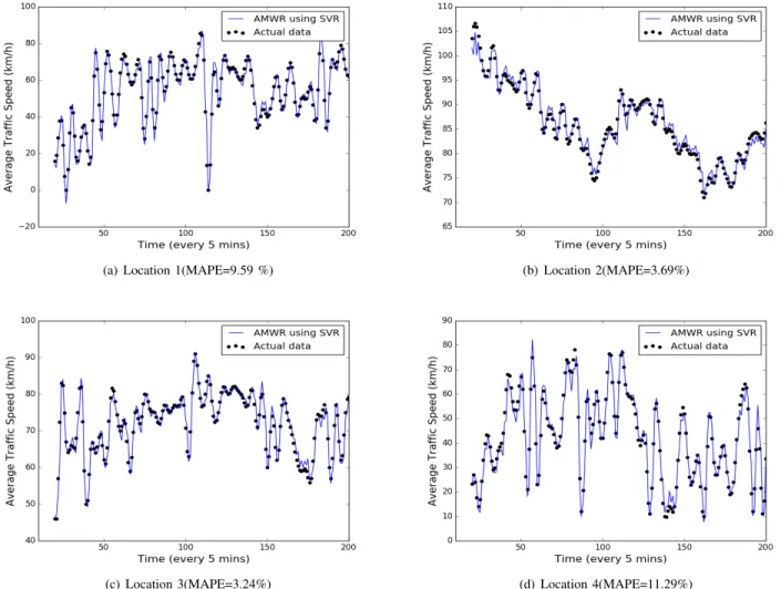
(a) Location 1(MAPE=9.59 %) (b) Location 2(MAPE=3.69%)
(c) Location 3(MAPE=3.24%) (d) Location 4(MAPE=11.29%) Fig. 5. Prediction results on average traffic speed data from four different locations.
TABLE I
ERROR ACCUMULATED OVER1MONTH PERIOD WITH DIFFERENT TRAINING WINDOW SIZE
No. Training window MAPE(%)
1 5 17.67 2 10 15.48 3 15 14.36 4 20 14.63 5 25 15.01 6 30 14.38 7 35 14.86 8 40 15.06 9 45 14.79 10 50 14.72
data streams as inputs. A more complex rule may involve other data sources like weather forecast or social media data. CEP generates a complex event when the average traffic speed and average traffic flow is less than the threshold values for 3 consecutive readings. Now if the input is predicted data as in our approach, the complex event detected will also be in the future and traffic administrators can take precautionary measures in order to avoid congestion. This is just one example that demonstrates how CEP rules can be exploited to find more
complex events.
Algorithm 2 Example Rule for CEP
for(speed, intensity)∈T upleW indow(3)do
2: if (speed(t) < speedthr and intensity(t) <
intensitythr AND
speed(t+ 1)< speedthr andintensity(t+ 1)<
intensitythr AND
4: speed(t+ 2)< speedthr andintensity(t+ 2)<
intensitythr)then
Generate complex event Bad Traffic 6: end if
end for
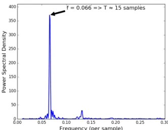
Four different sensing locations from city of Madrid were chosen randomly with different characteristics to get fair anal-ysis of the results. As described in section II, we applied the proposed Lomb Scargle method for finding optimum window size for training ML model. The resulting periodogram from one location for traffic speed is shown in the Figure 4. X-axis shows the frequency of data on per sample basis and y-axis represents the power spectral density. Data periodogram has a peak at 0.066 which corresponds to a window size
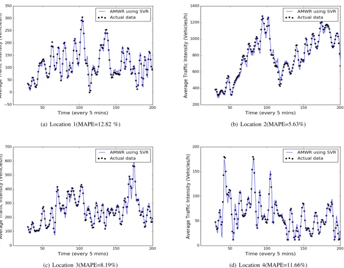
(a) Location 1(MAPE=12.82 %) (b) Location 2(MAPE=5.63%)
(c) Location 3(MAPE=8.19%) (d) Location 4(MAPE=11.66%) Fig. 6. Prediction results on average traffic intensity data from four different locations.
of 15 samples. We validated our method by using different window sizes for prediction on one month of traffic data and noted corresponding Mean Absolute Percentage Error (MAPE). MAPE is an accurate metric for evaluating the performance of prediction models and can be calculated as:
M AP E(%) = 1/n n X t=1 |(Yt−Y 0 t Yt )| ×100 (7)
where Yt represents actual data, Y 0
t represents predicted data and n represents the total number of predicted values. Table I shows the MAPE(%) for different window sizes and it can be seen that error is minimum when the window size of 15 samples or multiple of 15 is used which validates our approach.
Prediction results for traffic speed and traffic intensity data for all four locations is shown in Figure 5 and Figure 62. As it can be seen, that predicted values are tracking the actual data quite accurately. The reason behind it is that if there is an error in the predictions, it is incorporated and the model is updated accordingly and hence it prevents the error from propagating.
2Implementation Code and input data is available at https://github.com/
adnanakbr/predictive analytics
Finally, once we have the predicted values for traffic speed and traffic intensity, CEP can be used to infer traffic state using the rules mentioned in algorithm 2. Event detected by CEP will be in future providing enough time for traffic administrators to manage traffic pro-actively and avoiding congestion before it happens.
A. Performance Comparison
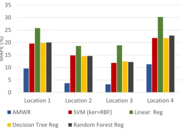
In order to compare the performance of AMWR with other regression models, we implemented several state-of-the-art regression algorithms available in python machine learning library scikit-learn [23]. Figure 7 and 8 shows the MAPE (%) plot of different regression algorithms implemented for all four locations , and Table II and III shows the results in tabular form. As it can be seen that AMWR outperforms other regression algorithms as it tracks the incoming data stream accurately. There are two main reasons for high accuracy provided by AMWR. 1) As new data arrive; AMWR takes the prediction error into account and retrain the model using more recent data. As the size of training window is very small, it is able to retrain and predict in near real-time.2) It tracks the error and if prediction error starts to increase, it decreases
the size of prediction window in order to maintain the level of accuracy. 0 5 10 15 20 25 30 35
Location 1 Location 2 Location 3 Location 4
M
AP
E
(%
)
AMWR SVM (ker=RBF) Linear Reg
Decision Tree Reg Random Forest Reg
Fig. 7. AMWR comparison with different models for traffic speed data
0 5 10 15 20 25 30 35 40 45
Location 1 Location 2 Location 3 Location 4
M
APE
(%
)
AMWR SVM (ker=RBF) Linear Reg
Decision Tree Reg Random Forest Reg
Fig. 8. AMWR comparison with different models for traffic intensity data
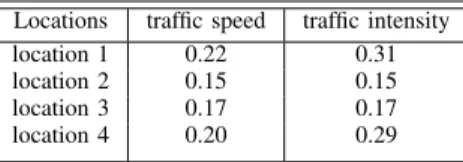
MAPE accumulated over a period of time is dependent on the data characteristics of underlying sensing location. If the data has more variations with a high value of standard deviation, the resulting accuracy on prediction readings will be lower. Table IV shows the input standard deviation for traffic speed and traffic intensity for all locations . Location 1 and location 4 have high standard deviation and hence high variance which resulted into more error as the spread of data points is effecting the predictions.
To further validate the performance of our prediction algo-rithm, we captured a congestion point in the input data for location 1. Figure 9 shows the comparison of AMWR based SVR with conventional SVR for predicting incoming data. As it can be seen in the figure that there is a congestion point after 170th minute when traffic speed suddenly drops to 0. A conventional SVR regression algorithm is unable to track the data whereas AMWR based SVR tracks the actual data
accurately and hence captures the congestion point.3
Fig. 9. Capturing a congestion event
TABLE II
MAPE(%)FOR TRAFFIC SPEED DATA
Method location 1 location 2 location 3 location 4
AMWR 9.59 3.69 3.24 11.29
SVM-RBF 19.57 14.83 11.84 21.84 Linear Reg 25.80 18.61 18.90 30.25 Decision Tree Reg 19.82 14.57 12.40 21.76 Random For Reg 20.04 14.63 12.22 22.80
TABLE III
MAPE(%)FOR TRAFFIC INTENSITY DATA
Method location 1 location 2 location 3 location 4
AMWR 12.82 5.63 8.19 11.66
SVM-RBF 33.20 19.70 22.94 31.61 Linear Reg 33.16 32.50 32.81 39.63 Decision Tree Reg 36.06 21.35 22.68 31.19 Random For Reg 36.53 21.25 22.85 31.73
B. Error Estimation
Overall error propagated through the system depends on the underlying CEP rule. As an example, consider the rule mentioned in algorithm 2. Equations 3-5 can be used to calculate the expression for overall error as:
pdfE(total) =n∗(pdfE(speed)∗pdfE(intensity)) (8) where n is the window length, pdfE(speed) is the proba-bility density function for speed error and pdfE(intensity) is probability density function for intensity error. If we have the generalized expressions for pdfE(speed) and
pdfE(intensity), they can be substituted in equation 8 to get an expression for the overall error of the system.
3Implementation Code and input data is available at https://github.com/
(a) Error distribution for traffic speed (location 1) (b) Error distribution for traffic intensity (location 1) Fig. 10. Error modeling for location 1
TABLE IV
INPUT STANDARD DEVIATION(σ) Locations traffic speed traffic intensity location 1 0.22 0.31 location 2 0.15 0.15 location 3 0.17 0.17 location 4 0.20 0.29
In order to get the probability of density functions for predicted traffic speed and traffic intensity, prediction error was calculated for one month data and plotted in the form of an histogram. An histogram is a graphical representation of the data which provides an estimation of the probability distribution of the data. Error distribution for traffic speed and traffic intensity for location 1 is shown in the Figure 10. Firstly, the Gaussian distribution was chosen to model the error propagation curve because of the bell shaped nature of the histogram as shown in figure 8. The probability density function for the Gaussian distribution is as follows:
pdfE(x) =
1 σ√2πe
−(x−µ)2/2σ2
(9)
whereµrepresents the mean andσrepresents the standard deviation of the distribution. The Gaussian distribution was ap-plied by using the curve fitting techniques and the parametric distribution for the error was found. The Gaussian distribution fitted well to model most of the data in error propagation histogram but it was ill-fitted for the outliers on the error histogram. Therefore a better fitted curve for error modeling was still needed.
The Student’s t distribution due to its heavy tail nature can better model the outliers. Also, the Student’s t distribution has a degree of freedom parameter which can be changed to tune the shape of the distribution according to the nature of error propagation data. Hence the Student’s t distribution can be used to further improve the modeling of error propagation data. The probability density function for Student‘s t-distribution is
TABLE V
ERROR DISTRIBUTION PARAMETERS FOR TRAFFIC INTENSITY
No. Gaussian distribution t-distribution location 1 µ= 0, σ= 0.27 ν= 1.79, µ= 0, σ= 0.13
location 2 µ= 0, σ= 0.21 ν= 1.90, µ= 0, σ= 0.10
location 3 µ= 0, σ= 0.22 ν= 1.73, µ= 0, σ= 0.10
location 4 µ= 0, σ= 0.26 ν= 1.67, µ= 0, σ= 0.12
TABLE VI
ERROR DISTRIBUTION PARAMETERS FOR TRAFFIC SPEED
No. Gaussian distribution t-distribution location 1 µ= 0, σ= 0.24 ν= 1.16, µ= 0, σ= 0.08 location 2 µ= 0, σ= 0.19 ν= 0.07, µ= 0, σ= 0.03 location 3 µ= 0, σ= 0.20 ν= 0.03, µ= 0, σ= 0.07 location 4 µ= 0, σ= 0.24 ν= 0.45, µ= 0, σ= 0.10 given by: pdfE(x) = Γ(ν+12 ) √ νπΓ(ν2) 1 + x 2 ν −ν+12 (10) whereν is the degrees of freedom parameter and Γ is the gamma function. The degrees of freedom parameterνcan tune the variance and leptokurtic nature of the distribution. With decreasing ν, the tails of the distribution becomes heavier. More details about the t-distribution can be found in [30][31]. Table V and VI shows the parameters for error distribution for both the Gaussian and Student’s t distribution at all four locations.
C. Large-Scale Implementation
In our proposed architecture, machine learning implemen-tation and evaluation has been done in python scikit-learn. Although it can support relatively large data-sets by scaling up but it is not very cost efficient and have certain limit on the amount of input data it can process. IoT has triggered a massive influx of big data and at city level solutions, we might potentially be analyzing data from hundreds of thousands of sensors. In order to overcome this issue and make our
solution truly scalable (scaling out in contrast to scaling up), we extended our work and implemented machine learning part in Spark MLlib which is machine learning library for Apache Spark [32].
Apache Spark is a general-purpose analytics engine that can process large amounts of data from various data sources and is gaining significant attraction in the big data domain. It performs especially well for iterative applications which include many machine learning algorithms. Spark maintains an abstraction called Resilient Distributed Datasets (RDDs) which can be stored in memory without requiring replication and are still fault tolerant. Moreover, Spark can analyze data from any storage system implementing the Hadoop FileSystem API, such as HDFS, Amazon S3 and OpenStack Swift. Further details about the large-scale implementation of our proposed solution can be found in [33] [34].
D. Other Use cases
Our proposed architecture provides a generic predictive solution for different IoT applications. Different components involved can easily be configured according to requirements of a specific application. Another example is smart health management in which different sensors are used to monitor patient’s health. These devices generate data at high rates and this data needs to be analyzed and correlated as soon as possible in order to ensure patient’s safety. If a patient’s heart beat or blood pressure starts to increase, our solution can detect the increasing trend and predict it in time before it reaches to dangerous level. CEP adds the capability to correlate the predictive readings with other data sources such as patient’s physical or eating activities in order to detect a possible complex event (health warning for patient).
The optimum window for training will be different for every data stream. And even though, many IoT data streams have some element of periodicity but nevertheless it is not always true. In such cases, we can define the default size for training window. The default size will be dependent on the requirements of the scenario as large training window will take more time in training. The definition of real time is scenario dependent, for instance in health monitoring scenario real time is under 10 seconds whereas for ITS a delay of 1-2 minutes will still be counted as real time. All the components used in our architecture are open source, easily available and can easily be made scalable for large scale applications.
IV. CONCLUSION ANDFUTUREWORK
In this paper, we have proposed and implemented an ar-chitecture for predicting complex events for proactive IoT applications. Our proposed architecture combines the power of real-time and historical data processing using CEP and ML respectively. We highlighted the common challenges for combining both technologies and implemented our proposed solution by addressing those challenges. In this regard, we proposed a prediction algorithm called AMWR for near real-time data. In contrast to conventional methods, it utilizes a moving window for training ML model enabling it to perform accurately for dynamic IoT data. The performance of the
prediction algorithm was validated on traffic data with an ac-curacy up to 96%. The feasibility of the proposed architecture was demonstrated with the help of a real-world use case from ITS where early predictions about the traffic state enables the system administrators to manage traffic in a better way.
Our experiments of using ML based predictions combined with CEP have shown an extra advantage on existing solutions by providing early warnings to traffic administrators about traffic events with high accuracy and given the generality of the proposed architecture, the same combination can also lead to better performances in other IoT scenarios such as monitoring goods in supply chain or smart health care. In future, we aim to evaluate our architecture for other IoT applications where early predictions about complex events can contribute to proactive solutions.
ACKNOWLEDGMENTS
The research leading to these results was supported by the EU FP7 project COSMOS under grant No 609043 and EU Horizon 2020 research project CPaaS.io under grant No 723076.
REFERENCES
[1] B. Yan and G. Huang, “Supply chain information transmission based on rfid and internet of things,” in2009 ISECS International Colloquium on Computing, Communication, Control, and Management, vol. 4, Aug 2009, pp. 166–169.
[2] L. Xiao and Z. Wang, “Internet of things: A new application for intelligent traffic monitoring system,”Journal of networks, vol. 6, no. 6, pp. 887–894, 2011.
[3] A. Akbar, M. Nati, F. Carrez, and K. Moessner, “Contextual occupancy detection for smart office by pattern recognition of electricity consump-tion data,” in2015 IEEE International Conference on Communications (ICC), June 2015, pp. 561–566.
[4] O. Etzion and P. Niblett,Event Processing in Action, 1st ed. Greenwich, CT, USA: Manning Publications Co., 2010.
[5] G. Cugola and A. Margara, “Processing flows of information: From data stream to complex event processing,” ACM Comput. Surv., vol. 44, no. 3, pp. 15:1–15:62, Jun. 2012. [Online]. Available: http://doi.acm.org/10.1145/2187671.2187677
[6] A. Akbar, F. Carrez, K. Moessner, J. Sancho, and J. Rico, “Context-aware stream processing for distributed iot applications,” inInternet of Things (WF-IoT), 2015 IEEE 2nd World Forum on, Dec 2015, pp. 663– 668.
[7] C. Y. Chen, J. H. Fu, T. Sung, P. F. Wang, E. Jou, and M. W. Feng, “Complex event processing for the internet of things and its applications,” in 2014 IEEE International Conference on Automation Science and Engineering (CASE), Aug 2014, pp. 1144–1149. [8] C.-H. Wu, J.-M. Ho, and D. T. Lee, “Travel-time prediction with support
vector regression,” IEEE Transactions on Intelligent Transportation Systems, vol. 5, no. 4, pp. 276–281, Dec 2004.
[9] H. xiang Zhao and F. Magouls, “A review on the prediction of building energy consumption,” Renewable and Sustainable Energy Reviews, vol. 16, no. 6, pp. 3586 – 3592, 2012. [Online]. Available: http://www.sciencedirect.com/science/article/pii/S1364032112001438 [10] C.-W. Tsai, C.-F. Lai, M.-C. Chiang, and L. T. Yang, “Data mining
for internet of things: a survey,”Communications Surveys & Tutorials, IEEE, vol. 16, no. 1, pp. 77–97, 2014.
[11] L. J. F¨ul¨op, ´A. Besz´edes, G. T´oth, H. Demeter, L. Vid´acs, and L. Farkas, “Predictive complex event processing: a conceptual framework for combining complex event processing and predictive analytics,” in Pro-ceedings of the Fifth Balkan Conference in Informatics. ACM, 2012, pp. 26–31.
[12] Y. Wang and K. Cao, “A proactive complex event processing method for large-scale transportation internet of things,” International Journal of Distributed Sensor Networks, vol. 2014, 2014.
[13] T. K. Moon, “The expectation-maximization algorithm,”Signal process-ing magazine, IEEE, vol. 13, no. 6, pp. 47–60, 1996.
[14] S. Nechifor, B. Trnauc, L. Sasu, D. Puiu, A. Petrescu, J. Teutsch, W. Waterfeld, and F. Moldoveanu, “Autonomic monitoring approach based on cep and ml for logistic of sensitive goods,” in IEEE 18th International Conference on Intelligent Engineering Systems INES 2014, July 2014, pp. 67–72.
[15] B. Thomas, F. Jose, S. Jordi, A. Almudena, and T. Wolfgang, “Real time traffic forecast,”Atos scientific white paper, vol. 2013, 2013. [16] G. Widmer and M. Kubat, “Learning in the presence of concept drift and
hidden contexts,”Machine learning, vol. 23, no. 1, pp. 69–101, 1996. [17] A. Valsamis, K. Tserpes, D. Zissis, D. Anagnostopoulos, and T.
Var-varigou, “Employing traditional machine learning algorithms for big data streams analysis: the case of object trajectory prediction,”Journal of Systems and Software, 2016.
[18] A. Bifet, G. Holmes, R. Kirkby, and B. Pfahringer, “Moa: Massive online analysis,”Journal of Machine Learning Research, vol. 11, no. May, pp. 1601–1604, 2010.
[19] M. Zaharia, T. Das, H. Li, S. Shenker, and I. Stoica, “Discretized streams: an efficient and fault-tolerant model for stream processing on large clusters,” inPresented as part of the, 2012.
[20] L. Bottou, “Large-scale machine learning with stochastic gradient de-scent,” inProceedings of COMPSTAT’2010. Springer, 2010, pp. 177– 186.
[21] A. Akbar, F. Carrez, K. Moessner, and A. Zoha, “Predicting complex events for pro-active iot applications,” inInternet of Things (WF-IoT), 2015 IEEE 2nd World Forum on, Dec 2015, pp. 327–332.
[22] Node-RED, “Node-RED: A visual tool for wiring the Internet of Things ,” http://nodered.org//, 2016, [Online; accessed 6-May-2016]. [23] F. Pedregosa, G. Varoquaux, A. Gramfort, V. Michel, B. Thirion,
O. Grisel, M. Blondel, P. Prettenhofer, R. Weiss, V. Dubourget al., “Scikit-learn: Machine learning in python,” The Journal of Machine Learning Research, vol. 12, pp. 2825–2830, 2011.
[24] W. H. Press and G. B. Rybicki, “Fast algorithm for spectral analysis of unevenly sampled data,”The Astrophysical Journal, vol. 338, pp. 277–280, 1989.
[25] M. A. Benjamin, R. A. Rigby, and D. M. Stasinopoulos, “Generalized autoregressive moving average models,”Journal of the American Sta-tistical Association, vol. 98, no. 461, pp. 214–223, 2003.
[26] A. J. Smola and B. Sch¨olkopf, “A tutorial on support vector regression,”
Statistics and computing, vol. 14, no. 3, pp. 199–222, 2004.
[27] Scouris, “Scouris‘s Arduino Adventures ,” https://scouris.wordpress. com/2010/09/10/temperature-sensing-with-arduino-php-and-jquery/, 2010, [Online; accessed 5-May-2016].
[28] N. P. Schultz-Møller, M. Migliavacca, and P. Pietzuch, “Distributed complex event processing with query rewriting,” in Proceedings of the Third ACM International Conference on Distributed Event-Based Systems, ser. DEBS ’09. New York, NY, USA: ACM, 2009, pp. 4:1– 4:12. [Online]. Available: http://doi.acm.org/10.1145/1619258.1619264 [29] G. Cugola, A. Margara, M. Matteucci, and G. Tamburrelli, “Introducing uncertainty in complex event processing: model, implementation, and validation,”Computing, vol. 97, no. 2, pp. 103–144, 2015. [Online]. Available: http://dx.doi.org/10.1007/s00607-014-0404-y
[30] K. L. Lange, R. J. Little, and J. M. Taylor, “Robust statistical modeling using the t distribution,”Journal of the American Statistical Association, vol. 84, no. 408, pp. 881–896, 1989.
[31] W. Rafique, S. M. Naqvi, P. J. B. Jackson, and J. A. Chambers, “Iva algorithms using a multivariate student’s t source prior for speech source separation in real room environments,” in 2015 IEEE International Conference on Acoustics, Speech and Signal Processing (ICASSP), April 2015, pp. 474–478.
[32] X. Meng, J. Bradley, B. Yavuz, E. Sparks, S. Venkataraman, D. Liu, J. Freeman, D. Tsai, M. Amde, S. Owenet al., “Mllib: Machine learning in apache spark,”Journal of Machine Learning Research, vol. 17, no. 34, pp. 1–7, 2016.
[33] COSMOS, “D.4.1.3. Information and Data Lifecycle Management: De-sign and open specification (Final) ,” http://iot-cosmos.eu/deliverablesl, 2016, [Online; accessed 6-April-2017].
[34] P. Ta-Shma, “Channeling Oceans of IoT Data ,” http://www.spark.tc/ channeling-oceans-of-iot-data/, 2016, [Online; accessed 6-April-2017].