Contents lists available atSciVerse ScienceDirect
Journal of Computational and Applied
Mathematics
journal homepage:www.elsevier.com/locate/cam
An efficient computational approach for multiframe blind deconvolution
Ying-Wai (Daniel) Fan
a, James G. Nagy
b,∗aGoogle Inc., Mountain View, CA, 94043, USA
bMathematics and Computer Science, Emory University, Atlanta, GA, 30322, USA
a r t i c l e i n f o Article history: Received 18 October 2010 Keywords: Astronomical imaging Blind deconvolution Gauss–Newton method Multiframe deconvolution Nonlinear inverse problem Variable projection
a b s t r a c t
Obtaining high resolution images of space objects from ground based telescopes involves using a combination of sophisticated hardware and computational post-processing techniques. An important, and often highly effective, computational post processing tool is multiframe blind deconvolution (MFBD). Mathematically, MFBD is modeled as a nonlinear inverse problem that can be solved using a flexible, variable projection optimization approach. In this paper we consider MFBD problems that are parameterized by a large number of variables. The formulas required for efficient implementation are carefully derived using the spectral decomposition and by exploiting properties of conjugate symmetric vectors. In addition, a new approach is proposed to provide a mathematical decoupling of the optimization problem, leading to a block structure of the Jacobian matrix. An application in astronomical imaging is considered, and numerical experiments illustrate the effectiveness of our approach.
©2011 Elsevier B.V. All rights reserved.
1. Introduction
Image restoration is the process of reconstructing an approximation of an image from blurred and noisy measurements. The image formation process is typically modeled as a convolution equation, where each pixel in the blurred image can be represented as a weighted average of pixels in the true image scene. The convolution kernel, which is also referred to as the point spread function (PSF), defines these weights, and the image formation (convolution) process is written as
Yk,ℓ
=
−
i,jHi,jXk−i,ℓ−j
+
Nk,ℓ,
(1)whereYk,ℓis a pixel of the observed image at the
(
k, ℓ)
position,Hi,jis the(
i,
j)
entry of the PSFH,Xk−i,ℓ−jis a pixel of the exact original image at the(
k−
i, ℓ
−
j)
position, andNk,ℓis additive noise. The PSF can sometimes be obtained by calibration of the optical instrument, or expressed by a mathematical formula. Eq.(1)can be written in matrix–vector form asy
=
Ax+
η
(2)whereyis a vector representing the observed, blurred and noisy image, andxis a vector representing the unknown true image we wish to reconstruct.Ais an ill-conditioned matrix defined by the point spread function,H.Amay be sparse and/or structured. For example, if the blur is spatially invariant and periodic boundary conditions are imposed, thenAhas a circulant matrix structure.
η
is a vector that represents unknown additive noise in the measured data.∗Corresponding author.
E-mail addresses:[email protected](Y.-W. Fan),[email protected](J.G. Nagy). 0377-0427/$ – see front matter©2011 Elsevier B.V. All rights reserved.
The termdeconvolutionis typically used when the PSF, or equivalently the matrixA, is known, whereasblind deconvolution
implies that the PSF, and hence matrixA, is not known. In the case of blind deconvolution it is necessary to use deblurring algorithms that can jointly estimate the PSF and the unknown true image scene. If we know a parametrized formula of the PSF, we can formulate the blind deconvolution problem as
y
=
A(
φ
)
x+
η
,
(3)where
φ
is a vector of some unknown parameters, andA(
φ
)
is the convolution matrix corresponding toφ
. For example, if we know the PSF is represented by a Gaussian function, with unknown mean(µ
1, µ
2)
and standard deviationσ
, we can takeφ
=
(µ
1, µ
2, σ )
and write the PSF asH
(
φ
)
i,j=
H(µ
1, µ
2, σ )
i,j=
1 2πσ
2e−(i−µ1)2+(j−µ2)2 2σ2
.
Often, as in this simple Gaussian blur example, there are far fewer parameters defining the PSF than pixels in the imagesx
andy. Efficient computational approaches have been developed for cases like this; see, for example, [1]. In this paper we consider the much more challenging situation where the number of parameters defining the PSF is approximately the same as the number of pixels in the image. Although parametrization may not substantially reduce the number of unknowns, it still serves as a strong constraint on the structure of the PSF.
In multiframe blind deconvolution (MFBD) [2–6], multiple images of the same object are obtained. Specifically, one obtains a set of (for example,m) observed images,
yi
=
A(
φ
i)
x+
η
i,
i=
1,
2, . . . ,
m,
(4)which can be put in our general discrete model(2)by setting
y
=
y1...
ym
,
φ
=
φ
1...
φ
m
,
η
=
η
1...
η
m
.
A common approach to solve the blind deconvolution problem, including the multiframe case, is to use a nonlinear least squares framework, min φ,x
f(
φ
,
x)
:= ‖
y−
A(
φ
)
x‖
22
.
(5)To solve this nonlinear least squares problem, we use the variable projection method, which eliminates the linear termx
and optimizes only over the nonlinear terms
φ
. The variable projection method is used in many nonlinear optimization problems with separable variables [7–12]. The approaches described in these papers can be used for small scale problems, or in situations where there are only a few nonlinear terms. In this paper we are interested in applications whereφ
may contain tens of thousands of parameters.The paper is organized as follows. We begin by describing the variable projection method for the single frame blind deconvolution problem in Section2, and then propose a decoupling approach for the multiframe problem in Section3. An example that arises in astronomical imaging is presented in Section4, and concluding remarks are given in Section5.
2. Variable projection and blind deconvolution
To solve the blind deconvolution problem, we would like to find PSF parameters
φ
and an approximation of the true imagexto minimize the functionf
(
φ
,
x)
= ‖
y−
A(
φ
)
x‖
22.
(6)One can note thatf depends on
φ
nonlinearly and onxlinearly. We apply the variable projection method to eliminate the linear variablex. The resulting projected function˜
f(
φ
)
is obtained by the following subproblem.˜
f(
φ
)
=
min x f(
φ
,
x)
=
min x‖
y−
A(
φ
)
x‖
22.
(7)The subproblem in(7)is a linear least squares problem. By simple numerical linear algebra, we know that the minimum of the subproblem is attained at
ˆ
x
=
A(
φ
)
Ďy,
whereA
(
φ
)
Ďis the pseudoinverse ofA(
φ
)
. Thus˜
If we enforce periodic boundary conditions, which is an appropriate assumption for applications in astronomical imaging, then the convolution matrixA
(
φ
)
has the spectral decomposition [13]A
(
φ
)
=
FH3(
φ
)
F,
whereFis the Fourier matrix and3
(
φ
)
is a diagonal matrix. IfH(
φ
)
of sizen×
nis the PSF corresponding toA(
φ
)
, then3
(
φ
)
=
Diag(
vec(
nfft(
H(
φ
)))) .
The matrixA
(
φ
)
is usually ill-conditioned, thus instead of takingA(
φ
)
Ďas the Moore–Penrose pseudoinverse, we use a regularized pseudoinverseA
(
φ
)
Ď=
(
A(
φ
)
HA(
φ
)
+
α
2)
−1A(
φ
)
H=
FH 3(
φ
)
|
3(
φ
)
|
2+
α
2F,
where
α
is a regularization parameter. Here we use the shorthand notationα
2in place ofα
2I, and arithmetic operations between diagonal matrices to mean elementwise operations on the diagonal entries. We remark that choosing the regularization parameter is a nontrivial issue, and is not one that we address in this paper. Our aim is to show that if an appropriate value ofα
is known, then we can efficiently implement a Gauss–Newton method for the MFBD problem. Some discussion of choosing the regularization parameter in the context of blind deconvolution can be found in [1] and references therein.For notational convenience, we drop ‘‘
(
φ
)
’’ in equations henceforth. We also use the notationP
=
AAĎ=
FH|
3|
2|
3|
2+
α
2F and P⊥=
I−
P=
I−
AAĎ=
FHα
2|
3|
2+
α
2F.
(9)With this notation and(8), the minimization problem can be reposed as min φ
˜
f(
φ
)
:= ‖
P⊥(
φ
)
y‖
22
.
(10)Eq.(10)is a nonlinear least squares problem. We use the Gauss–Newton algorithm, with conjugate gradients for the inner iterations, to solve this problem; see Algorithm 1.
Algorithm 1Solving the blind deconvolution problem by Gauss–Newton algorithm with conjugate gradient as the inner solver
whilenot convergeddo
Solve the normal equations
J
(
φ
)
HJ(
φ
)
p= −
J(
φ
)
Hr,
(
11)
where
r
=
y−
A(
φ
)
x=
P⊥(
φ
)
y,
J
= ∇
(
P⊥(
φ
)
y)
= ∇
P⊥(
φ
)
y,
(
12)
for the search directionpby conjugate gradient method.
Set
φ
⇐
φ
+
β
p, whereβ
is chosen using a line search on minimizing‖
r‖
2.end while
Setx
⇐
A(
φ
)
Ďy.The
∇
in (12) denotes differentiation with respect toφ
. Thus∇
P⊥is a three-dimensional tensor. Care must be takenwhen computing the multiplication of
∇
P⊥y: the inner product is done along the second dimension of∇
P⊥.In general, multiplication of a three-dimensional tensor to a vector takesO
(
N3)
operations, whereN=
n2is the number of pixels in the image. Using the spectral decomposition of∇
P⊥and the special property of our test problem (to be discussed in Section4), we can reduce the complexity down to justO(
NlogN)
. We prove in theAppendixthat∇
1|
3|
2+
α
2
= −
2 Re
3∇
3
(
|
3|
2+
α
2)
2,
(13)where Re
(
·
)
returns the real part of a complex matrix or tensor. Then from(9),∇
P⊥=
α
2FH∇
1|
3|
2+
α
2
F= −
2α
2FH Re
3∇
3
(
|
3|
2+
α
2)
2F.
Therefore, the Jacobian matrixJhas the spectral decomposition: J
= ∇
P⊥y= −
2α
2FH Re
3∇
3
(
|
3|
2+
α
2)
2Fy (14)= −
2α
2FH Re
3∇
3
(
|
3|
2+
α
2)
2yˆ
.
(15)Here we usey
ˆ
to denote the Fourier transform ofy. Again, the tensor–vector products in(14)are(15)are done along the second dimension of the tensor Re
3∇
3
. Since 3is diagonal, the tensor Re
3∇
3
essentially has only two dimensions.We note that(15)only involves the Fourier matrixF, a diagonal matrix3and a ‘‘diagonal’’ tensor
∇
3. Multiplication byF
,
3and∇
3can be done respectively inO(
NlogN)
(by fast Fourier transform [14,15]),O(
N)
, andO(
NlogN)
(to be shown in Section4.1).With the identities established so far, we see that the left hand side of Eq. (11) can be written as
JHJp
=
−
2α
2FH Re
3∇
3
(
|
3|
2+
α
2)
2yˆ
H
−
2α
2FH Re
3∇
3
(
|
3|
2+
α
2)
2yˆ
p=
4α
4
ˆ
yH Re
(
∇
3)
T3
(
|
3|
2+
α
2)
2 FF H Re
3∇
3
(
|
3|
2+
α
2)
2yˆ
p=
4α
4
ˆ
yH Re
(
∇
3)
T3
Re
3∇
3
(
|
3|
2+
α
2)
4 yˆ
p,
while the right hand side of Eq. (11) is given by
−
JHr= −
JHP⊥y= −
−
2α
2FH Re
3∇
3
(
|
3|
2+
α
2)
2yˆ
H
FHα
2|
3|
2+
α
2Fy=
2α
4yˆ
H Re
(
∇
3)
T3
(
|
3|
2+
α
2)
2 FF H 1|
3|
2+
α
2yˆ
=
2α
4yˆ
H Re
(
∇
3)
T3
(
|
3|
2+
α
2)
3 yˆ
.
Hence Eq. (11) is reduced to4
α
4
ˆ
yH Re
(
∇
3)
T3
Re
3∇
3
(
|
3|
2+
α
2)
4 yˆ
p=
2α
4yˆ
H Re
(
∇
3)
T3
(
|
3|
2+
α
2)
3 yˆ
2
ˆ
yHRe
(
∇
3)
T3
Re
3∇
3
(
|
3|
2+
α
2)
4 yˆ
p= ˆ
yH Re
(
∇
3)
T3
(
|
3|
2+
α
2)
3 yˆ
.
(16)To make this equation clearer, we use
∇
k3to denotedd3φkandpjto denote thej-th component ofp.
1Thei-th components of both sides of(16)are then given by
−
j
2yˆ
H Re
∇
i3T3
Re
3∇
j3
(
|
3|
2+
α
2)
4 yˆ
pj= ˆ
yH Re
∇
i33
(
|
3|
2+
α
2)
3yˆ
(17) and 2yˆ
H Re
∇
i3T3
(
|
3|
2+
α
2)
2−
j
Re
3∇
j3
(
|
3|
2+
α
2)
2yˆ
pj= ˆ
yH Re
∇
i33
(
|
3|
2+
α
2)
3yˆ
.
(18)If we use the notation
˜
yi=
Re
3∇
i3
(
|
3|
2+
α
2)
2yˆ
and yˇ
=
1|
3|
2+
α
2yˆ
,
then Eq.(17)can be further reduced to2y
˜
iH−
j˜
yjpj
= ˜
yHi yˇ
.
The Gauss–Newton algorithm with the simplified formula is shown in Algorithm 2.
Algorithm 2Solving the blind deconvolution problem by Gauss–Newton algorithm with conjugate gradient as the inner solver using the simplified formula
whilenot convergeddo
Solve the normal equations 2y
˜
iH−
j˜
yjpj= ˜
yiHyˇ
,
i=
1,
2, . . . ,
N(
19)
where˜
yi=
Re
3(
φ
)
∇
i3(
φ
)
(
|
3(
φ
)
|
2+
α
2)
2ˆ
yˇ
y=
1|
3(
φ
)
|
2+
α
2yˆ
,
(
20)
by the conjugate gradient method for the search directionp.
Set
φ
⇐
φ
+
β
p, whereβ
is chosen using a line search on minimizing‖
r‖
2.end while
Setx
⇐
A(
φ
)
Ďy.When solving the normal equations in (19) by the conjugate gradient method, we need to do the multiplications
∑
jy˜
jpj and[ ˜
yHi y
ˇ
]
ni=1efficiently. To describe how this is done, recall that a vectoruof lengthnis calledconjugate symmetricif
u1is real
uk
=
un−k+2 fork=
2, . . . ,
n.
It is a well-known fact that Fourier transforms of real vectors are conjugate symmetric. Furthermore, ifuandvare conjugate symmetric vectors, then
uTv
=
uTvand
Re
(
u)
Tv=
uTRe(
v) .
In the following, we use the assumptions thatpis a real vector andy
ˇ
is a conjugate symmetric vector. In addition, we denote by Diag(
v)
the diagonal matrix whose diagonal entries are given by the vectorv, and diag(
D)
is a vector whose entries are given by the diagonal elements of the matrixD(notice the difference in our use of the upper caseDiagoperator and the lower casediagoperator).From the identityDv
=
Diag(
v)
diag(
D)
, we have∇
j3yˆ
=
Diag
yˆ
∇
jdiag(
3)
⇒ ∇
3yˆ
=
Diag
yˆ
∇
diag(
3) .
Using this property we see that−
j˜
yjpj=
−
j Re
3∇
j3
(
|
3|
2+
α
2)
2yˆ
pj=
Re
3∇
3
(
|
3|
2+
α
2)
2yˆ
p=
Diag
ˆ
y
(
|
3|
2+
α
2)
2Re
3∇
diag(
3)
p=
Diag
ˆ
y
(
|
3|
2+
α
2)
2Re
3∇
diag(
3)
p
.
(21)Eq.(21)is due to the assumption thatpis real. Computing
∑
jy
˜
jpjas in(21)has the advantage that operations can be done from right to left: first compute∇
diag(
3)
p, then3∇
diag(
3)
pand so on. Each intermediate step returns a vector of the same size, thus the need for extra temporary memory is minimized. Also the matrices involved are diagonal matrices except∇
diag(
3)
, so each step can be done very cheaply, except possibly the step with∇
diag(
3)
, which is application dependent. Then for[ ˜
yH i p]
ni=1, we consider[ ˜
yiHyˇ
]
ni=1=
Re
3∇
i3
(
|
3|
2+
α
2)
2yˆ
H
ˇ
y
n i=1=
Re
3∇
3
(
|
3|
2+
α
2)
2yˆ
H
ˇ
y=
Diag
yˆ
(
|
3|
2+
α
2)
2Re
3∇
diag(
3)
H
ˇ
y=
Re
∇
diag(
3)
3
Diag
ˆ
y
(
|
3|
2+
α
2)
2yˇ
= ∇
diag(
3)
3Re
Diag
ˆ
y
(
|
3|
2+
α
2)
2yˇ
.
(22)Eq.(22)is due to the assumption thaty
ˇ
is conjugate symmetric. Again, computing[ ˜
yHi y
ˇ
]
ni=1as in(22)has the advantage that operations can be done from right to left, and the matrices involved are diagonal matrices except∇
diag(
3)
.In Section4.1, we discuss how to compute multiplications with
∇
diag(
3)
and its transpose efficiently for a specific application in astronomical imaging.3. Multiframe blind deconvolution
The MFBD problem can be formulated as the nonlinear least squares problem
min φ,x
y1 y2...
ym
−
A(
φ
1)
A(
φ
2)
...
A(
φ
m)
x
2 2.
(23)We can try to use variable projection to eliminatexby substituting
x
=
A(
φ
1)
A(
φ
2)
...
A(
φ
m)
Ď
y1 y2...
ym
and obtain min φ
I−
A(
φ
1)
A(
φ
2)
...
A(
φ
m)
A(
φ
1)
A(
φ
2)
...
A(
φ
m)
Ď
y1 y2...
ym
2 2.
(24)We can then proceed as in Section2with the Gauss–Newton algorithm. This, however, has several drawbacks. The formula for the pseudoinverse in(24)is complicated. Because of the coupling of theA
(
φ
i)
in the pseudoinverse, the Jacobian matrix has an even more complicated formula and it is dense.To get a simpler formula and for more efficient implementation, we reformulate the minimization problem(23)through a decoupling scheme. In particular, we solve each of the individual blind deconvolution problems, allowing reconstruction
of different objectsxi. However, since eachxishould actually be identical, we include additional constraints that minimize the difference betweenxiandxi+1. Specifically, we solve the minimization problem
min
‖
y1−
A(
φ
1)
x1‖
22+ ‖
y2−
A(
φ
2)
x2‖
22+ · · · + ‖
ym−
A(
φ
m)
xm‖
22+ ‖
x1−
x2‖
22+ ‖
x2−
x3‖
22+ · · · + ‖
xm−1−
xm‖
22+ ‖
xm−
x1‖
22,
(25) wherexi
=
A(
φ
i)
Ďyi.
Eq.(25)can be rewritten asmin
‖
r‖
22,
(26) where r=
y1−
A(
φ
1)
x1 y2−
A(
φ
2)
x2...
ym−
A(
φ
m)
xm x1−
x2 x2−
x3...
xm−1−
xm xm−
x1
.
(27)This decoupling idea is similar to an approach used in [16] to solve the deblurring and denoising problem with total variation regularization.
We use the following notations.
Ji
= ∇
φi
yi−
A(
φ
i)
xi
= ∇
φi
P⊥(
φ
i)
yi
= −
2α
2FH Re
3i∇
3i
(
|
3i|
2+
α
2)
2yˆ
i= −
2α
2FH Diag
ˆ
yi
(
|
3i|
2+
α
2)
2Re
3i∇
diag(
3i)
,
(28) and Ki= ∇
φixi= ∇
φi
A(
φ
i)
Ďyi
= ∇
φi
FH 3i|
3i|
2+
α
2Fyi
=
FH∇
φi
3i|
3i|
2+
α
2
Fyi=
FHα
2∇
3 i−
3i 2∇
3i(
|
3i|
2+
α
2)
2 yˆ
i (29)=
FH Diag
ˆ
yi
(
|
3i|
2+
α
2)
2
α
2∇
diag(
3 i)
−
3i 2∇
diag(
3i)
,
(30) whereA(
φ
i)
=
FH3iF. In(29), we use the identity
∇
3|
3|
2+
α
2
=
α
2∇
3−
32∇
3(
|
3|
2+
α
2)
2,
(31)The Jacobian matrix of(26)has the form of J
=
J1 J2...
...
Jm K1−
K2 K2−
K3...
...
Km−1−
Km−
K1 Km
.
(32)With the decoupling formulation, the multi-frame blind deconvolution problem can be solved by the Gauss–Newton algorithm (Algorithm 3).
Algorithm 3Solving the multi-frame blind deconvolution problem by Gauss–Newton algorithm with conjugate gradient as the inner solver
whilenot convergeddo
Solve the normal equations
JHJp
= −
JHr,
(
33)
whereris given by (27) andJis given by (28), (30) and (32), for the search directionpby the conjugate gradient method.
Set
φ
1φ
2...
φ
m
⇐
φ
1φ
2...
φ
m
+
β
p, whereβ
is chosen using a line search on minimizing‖
r‖
2.end while Setx
=
A(
φ
1)
A(
φ
2)
...
A(
φ
m)
Ď
y1 y2...
ym
.When solving the normal equations (33) in Algorithm 3 with the conjugate gradient method, we need to multiplyJand
JHto vectors. From(32), we see thatJhas a block diagonal structure, and these operations can be done very efficiently; for details, see [17].
Finally we remark that recognizing convergence of the Gauss–Newton iteration is a nontrivial topic for inverse problems such as MFBD. Note that we incorporate Tikhonov regularization for the linear termx, but for the nonlinear term
φ
we use the stopping iteration as a form or regularization. More specifically, if an estimate of the noise is known, then the discrepancy principle can be used to estimate an appropriate stopping iteration; see, for example [18].4. Application to astronomical imaging
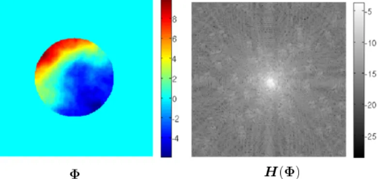
In this section we describe a specific application in astronomical imaging. Given the pupil phase function8, which describes the wavefront at the pupil of a telescope, the PSF is defined by
H
= |
ifft
eı8
|
2.
(34)We useıto denote
√
−
1,
ifft(
X)
to denote the inverse 2D FFT ofXand the exponential function in(34)is done elementwise. An example of a pupil phase function and its corresponding PSF is shown inFig. 1. In this and subsequent figures of PSFs, the logarithms of the PSFs are shown instead of PSFs themselves for better contrast. Values of the pupil phase function8 are zero outside the pupil, hence we only need to consider those values of8inside the pupil.In the test problem used in this section,8is of size 256
×
256, with a total of 65 536 elements. After discarding elements outsides the pupil, we still have 12 851 elements. Recall from Section3, in blind deconvolution we are minimizingf
(
φ
,
x)
=
min φ,xFig. 1. A pupil phase function,8, and its corresponding point spread functionH(8).
where
φ
=
vec(
8)
. In our test problem, the original imagexand the blurred imageyeach contains 65 536 elements. The joint minimization is over space of dimension 65 536+
12 851=
78 387 using 65 536 data values. Using variable projection, we instead are minimizing˜
f
(
φ
)
= ‖
(
I−
A(
φ
)
A(
φ
)
Ď)
y‖
22.
The dimension of the search space drops to 12 851, but this still is a very large number compared to other problems in the literature that use the variable projection method, in which only a few parameters (e.g., 3) remain after projection.
4.1. Efficient computations with
∇
diag(
3)
From Sections2and3, we know that efficient application of Gauss–Newton algorithms depends on an efficient way to do multiplication with
∇
diag(
3)
. We now derive the formula for∇
diag(
3)
for the specific case when the PSF has the form given in(34).As in earlier sections of this paper, we useFto denote the 2D unitary FFT matrix acting on vectorized matrices, andekto denote the unit vector with 1 at thek-th position and 0 at other positions. We use ‘‘
.
∗
’’ to denote elementwise multiplication.With these notations, the convolution matrixAcorresponding to the PSFh
=
vec(
H)
is given byA
=
FH3F,
with 3=
Diag
√
NFh
,
(35)whereNis the number of elements inh. We let
ϕ
=
eıφ.
Then dϕ
dφ
k=
ıϕ
kek.
The formula(34)forhcan be rewritten as
h
=
FHϕ
.
∗
FHϕ
.
Differentiatinghwith respect to an entry
φ
kofφ
, we havedh d
φ
k=
FH dϕ
dφ
k.
∗
FHϕ
+
FHϕ
.
∗
FH dϕ
dφ
k=
2 Re
FHϕ
.
∗
FH dϕ
dφ
k
=
2 Re
FHϕ
.
∗
FHıϕ
kek
=
2 Re
−
ıFHϕ
.
∗
FHϕ
kek
=
2 Im
FHϕ
.
∗
FHϕ
kek
,
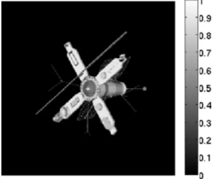
(36)Fig. 2. The original unblurred satellite image.
where Im
(
·
)
returns the imaginary part of a complex matrix. It follows from(36)thatdh d
φ
=
2 Im
FHϕ
.
∗
FHDiag(
ϕ
)
=
2 Im
FHϕ
.
∗
FDiag(
ϕ
)
.
(37) From(35)and(37),∇
diag(
3)
= ∇
(
√
NFh)
=
√
NFdh dφ
=
2√
NFIm
FHϕ
.
∗
FDiag(
ϕ
)
=
2√
NFIm
Diag
FHϕ
FDiag(
ϕ
)
.
(38) Now we multiply∇
diag(
3)
to a real vectorp.∇
diag(
3)
p=
2√
NFIm
Diag
FHϕ
FDiag(
ϕ
)
p=
2√
NFIm
Diag
FHϕ
FDiag(
ϕ
)
p
.
(39)The above multiplication(39)can then be done from right to left: first compute Diag
(
ϕ
)
p, thenFDiag(
ϕ
)
pand so on. Each intermediate step returns a vector of the same size, thus the need for extra temporary memory is minimized. Also each intermediate step involves only a diagonal or Fourier matrix, so each step can be done very cheaply.Now we multiply
(
∇
diag(
3))
Tto a conjugate symmetric vectorq.(
∇
diag(
3))
Tq=
2√
NIm
Diag(
ϕ
)
FDiag
FHϕ
Fq=
2√
NIm
Diag(
ϕ
)
FDiag
FHϕ
Fq
.
(40) Eq.(40)uses the fact thatFqis real. Again,(40)can be done from right to left, with each intermediate step involving only a diagonal or Fourier matrix, and the result is a vector of the same size.4.2. Experimental results
We test the Gauss–Newton algorithm with variable projection on a satellite image (Fig. 2). First we blur the satellite image by the PSFs of three pupil phase functions, and then deblur using a different number of blurred images. These test data were provided to us by Stuart Jefferies from the Institute of Astronomy, University of Hawaii.
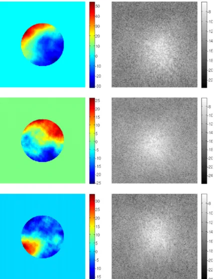
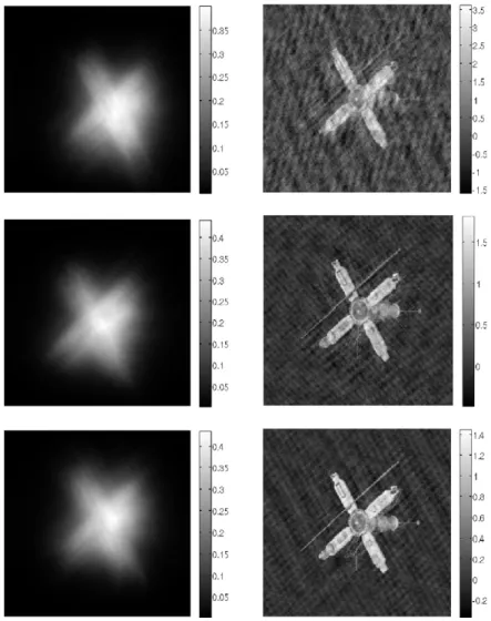
The three pupil phase functions and their corresponding PSFs used in this experiment are shown inFig. 3. After blurring the satellite image with the three PSFs, we have three blurred images (left hand side ofFig. 4). We now try to deblur them. Our initial guesses of pupil phase functions are obtained by adding 10% random noise to the true pupil phase functions. The right column inFig. 4shows the deblurred images using the initial guess. The initial deblurred images are sharper than the starting blurred images, but artifacts spread throughout the whole image and the pixel values lie in the wrong range.
Next, we deblur the blurred images using one (with Algorithm 2), two and three frames (with Algorithm 3) and compare the results. With just one frame, we do not get back a clear image (Fig. 5), although most artifacts are gone and pixel values are in the correct range. The relative error for this case is 0.4645. If we use two frames, a clearer image (Fig. 6) is obtained, but we still have some artifacts. The relative error has improved by a little to 0.3104. Further improvement
Fig. 3. The pupil phase functions and their corresponding point spread functions giving severe blurs.
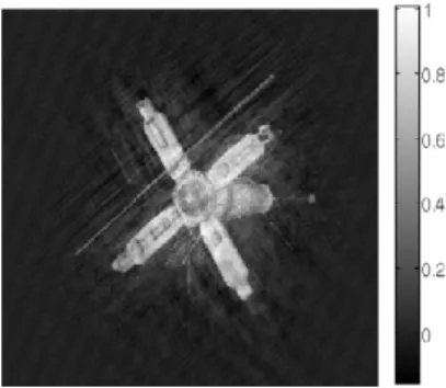
is observed when we use all three frames. The deblurred image (Fig. 7) is very sharp and the relative error is now just 0.1222.
These experimental results illustrate the success of the variable projection method in reducing the number of variables, and the effectiveness of the Gauss–Newton method in minimizing the projected objective function. The results also show that using multiple frames can significantly improve the blind deconvolution quality. Although we have considered a specific MFBD application, the basic optimization approach can be applied in other situations. The quality of the results depends on several factors, including the initial guess. As discussed in the paper, in the astronomical imaging application considered here, there are approaches where a good initial guess can be obtained.
5. Concluding remarks
In this paper we investigated the blind deconvolution problem for images affected by pupil phase atmospheric blurs common in astronomical imaging. In many blind deconvolution problems, the PSFs are parametrized to reduce the number of variables. But unlike common blurs like Gaussian, motion and out-of-focus blurs, the number of parameters of an atmospheric blur described by a pupil phase function is of the order of 10 000 for images of size 256
×
256. Together with the linear variables (the unknown image), the total number of variables is more than 70 000. The variable projection approach eliminates the linear terms, but the reduced cost functional still requires optimizing over the nonlinear terms defined by the pupil phase function. Compared with many problems in the literature solved by variable projection, our problem has significantly more variables, even after the projection.In the multiframe problems, we decoupled the frames into separate deblurring problems, with the constraint that the deblurred images should be close to each other, and obtained a sparse, block structured Jacobian matrix. The block structure
Fig. 4. Left: images obtained by blurring with the three point spread functions inFig. 3. Right: the deblurring results using the initial guess of the pupil phase functions.
Fig. 5. Deblurring result using only one image. Relative error=0.4645.
significantly reduces the storage requirements, and allows for parallel implementation of the Jacobian matrix–vector multiplications.
Of course one could use a low storage scheme, such as gradient descent or nonlinear conjugate gradients to solve the nonlinear least squares problem. This avoids the need to solve the Jacobian system, but it then may require 1000 or more iterations compared to the approximately 30 Gauss–Newton iterations used in our experiments. The efficiency with which we are able to solve the Jacobian system, combined with a structure that is highly amenable to parallel implementation, makes the Gauss–Newton approach highly competitive.
Fig. 6. Deblurring result using two images. Relative error=0.3104.
Fig. 7. Deblurring result using three images. Relative error=0.1222.
Acknowledgments
The second author’s research was supported by the United States National Science Foundation (NSF) under grant DMS-0811031, and by the United States Air Force Office of Scientific Research (AFOSR) under grant FA9550-09-1-0487.
Appendix
In this section we provide derivations of the formulas given in Eqs.(13)and(31). First we determine a formula for
∇|
3|
2.∇|
3|
2= ∇
(
33)
= ∇
33+
3∇
3= ∇
33+
3∇
3=
3∇
3+
3∇
3=
2 Re
3∇
3
.
We also need to use the following identity on derivatives of matrix inverses. Assume thatAis a matrix in which each entry is a function of a scalarx. Then
dA−1
dx
= −
A−1dA
dxA
−1
.
To establish the identity in Eq.(13), consider
d d
φ
k
1|
3|
2+
α
2
=
d dφ
k(
|
3|
2+
α
2)
−1= −
(
|
3|
2+
α
2)
−1 d dφ
k
|
3|
2+
α
2
(
|
3|
2+
α
2)
−1= −
(
|
3|
2+
α
2)
−2 d dφ
k
|
3|
2+
α
2
= −
(
|
3|
2+
α
2)
−2 d dφ
k(
|
3|
2).
Note that in the above calculations, we use the fact that diagonal matrices commute. Finally,
∇
1|
3|
2+
α
2
= −
(
|
3|
2+
α
2)
−2∇
(
|
3|
2)
= −
(
|
3|
2+
α
2)
−2
2 Re
3∇
3
= −
2 Re
3∇
3
|
3|
2+
α
2
2.
To establish the identity in Eq.(31), use the product rule and the above relationships, and obtain
∇
3|
3|
2+
α
2
= ∇
1|
3|
2+
α
23
= ∇
1|
3|
2+
α
2
3+
1|
3|
2+
α
2∇
3= −
|
3|
2+
α
2
−2
2 Re
3∇
3
3+
|
3|
2+
α
2
−1∇
3=
|
3|
2+
α
2
−2
−
(
3∇
3+
3∇
3)
3+
|
3|
2+
α
2
∇
3
=
|
3|
2+
α
2
−2
−
32∇
3− |
3|
2∇
3+ |
3|
2∇
3+
α
2∇
3
=
|
3|
2+
α
2
−2
−
32∇
3+
α
2∇
3
=
α
2∇
3−
32∇
3(
|
3|
2+
α
2)
2.
References[1] J. Chung, J.G. Nagy, An efficient iterative approach for large-scale separable nonlinear inverse problems, SIAM Journal on Scientific Computing 31 (2010) 4654–4674.
[2] R.G. Lane, Blind deconvolution of speckle images, Journal of the Optical Society of America A 9 (1992) 1508–1514. [3] N.F. Law, D.T. Nguyen, Multiple frame projection based blind deconvolution, Electronics Letters 31 (1995) 1734–1735.
[4] M.G. Löfdahl, Multi-frame blind deconvolution with linear equality constraints, in: F.M. Bones (Ed.), Image Reconstruction from Incomplete Data II, vol. 4792–21, SPIE, 2002.
[5] C.L. Matson, K. Borelli, S. Jefferies, C.C. Becnker, E.K. Hege, M. Lloyd-Hart, Fast and optimal multiframe blind deconvolution algorithm for high-resolution ground-based imaging of space objects, Applied Optics 48 (2009) A75–A92.
[6] N. Miura, N. Baba, Segmentation-based multiframe blind deconvolution of solar images, Journal of the Optical Society of America A 12 (1995) 1858–1866.
[7] G. Golub, V. Pereyra, The differentiation of pseudo-inverses and nonlinear least squares problems whose variables separate, SIAM Journal on Numerical Analysis 10 (2) (1973) 413–432.
[8] L. Kaufman, A variable projection method for solving separable nonlinear least squares problems, BIT Numerical Mathematics 15 (1) (1975) 49–57. [9] M.R. Osborne, Some special nonlinear least squares problems, SIAM Journal on Numerical Analysis 12 (4) (1975) 571–592.
[10] A. Ruhe, P.A. Wedin, Algorithms for separable nonlinear least squares problems, SIAM Review 22 (3) (1980) 318–337.
[11] G. Golub, V. Pereyra, Separable nonlinear least squares: the variable projection method and its applications, Inverse Problems 19 (2003) R1–R26. [12] M.R. Osborne, Separable least squares, variable projection, and the Gauss–Newton algorithm, Electronic Transactions on Numerical Analysis 28 (2007)
1–15.
[13] P.C. Hansen, J.G. Nagy, D.P. O’Leary, Deblurring Images: Matrices, Spectra, and Filtering, SIAM, Philadelphia, 2006. [14] C.F. Van Loan, Computational Frameworks for the Fast Fourier Transform, SIAM, Philadelphia, 1992.
[15] J. Cooley, J. Tukey, An algorithm for the machine calculation of complex Fourier series, Mathematics of Computation 19 (90) (1965) 297–301. [16] Y.-W. Wen, M.K. Ng, W.-K. Ching, Iterative algorithms based on decoupling of deblurring and denoising for image restoration, SIAM Journal on Scientific
Computing 30 (5) (2008) 2655–2674.
[17] Y.W. Fan, Practical image deblurring with synthetic boundary conditions, with gpus, and with multiple frames, Ph.D. Thesis, Emory University University, Atlanta, GA, 2010.