Tree Boosting Data Competitions with XGBoost

(1)

Title: Tree Boosting Data Competitions with XGBoost Author: Carlos Bort Escabias

Advisor: Pedro Delicado

Department: Deptartament d’Estadística I Investigació Operativa

University: Universitat Politècnica de Catalunya - Universitat de Barcelona

Academic year: 2016-2017

in Statistics and

Operations Research

(2)

(3)

Facultat de Matem`

atiques i Estad´ıstica

Master’s Thesis

Tree Boosting Data Competitions with

XGBoost

Carlos Bort Escabias

Director: Dr. Pedro _Delicado

(4)

(5)

This Master’s Degree Thesis objective is to provide understanding on how to approach a super-vised learning predictive problem and illustrate it using a statistical/machine learning algorithm, Tree Boosting. A review of tree methodology is introduced in order to understand its evolution, since Classification and Regression Trees, followed by Bagging, Random Forest and, nowadays, Tree Boosting. The methodology is explained following the XGBoost implementation, which achieved state-of-the-art results in several data competitions. A framework for applied predictive modelling is explained with its proper concepts: objective function, regularization term, overfit-ting, hyperparameter tuning, k-fold cross validation and feature engineering. All these concepts are illustrated with a real dataset of videogame churn; used in a datathon competition.

(6)

(7)

1 Introduction 4 1.1 Objective . . . 4 1.2 Supervised Learning . . . 6 1.3 Elements of a datathon . . . 7 1.4 Why XGBoost? . . . 8 1.5 Notation . . . 9 2 Prediction methods 11 2.1 Tree models . . . 11 2.1.1 Bagging . . . 14 2.1.2 Random Forest . . . 14 2.1.3 Tree Boosting . . . 15

2.2 Split finding algorithms . . . 19

2.3 Evaluation metrics . . . 22

3 Data splitting and Parameter tuning 24 3.1 Overfitting . . . 24

3.2 Model tuning . . . 25

3.3 k-fold cross validation . . . 26

4 Data and description 27 4.1 Descriptive . . . 27

4.2 Feature Engineering . . . 28

5 Hands on XGBoost 30 5.1 Parameters . . . 30

5.1.1 Parameters for Tree Booster . . . 31

5.1.2 Learning Task Parameters . . . 32

5.2 Training & Parameter tuning . . . 33

6 Conclusions and further research 37

Bibliography 39

(8)

Tree Boosting Data Competitions with XGBoost

A Grid Search by multiple parameters 42

B XGBoost parameter tuning 43

C Train by XGBoost 46

(9)

Introduction

1.1 Objective

Many of our current day by day digital decisions are made by machines, such as deciding which emails are classified as spam, which items are presented in a website, the grant of a credit, how to classify a website comment, among others. Nowadays these decisions are under the scope of machine learning: algorithms trained by humans to recognize patterns and make decisions. The main objective of this thesis is to understand how to approach a supervised learning predictive problem and review one of the machine learning techniques that shines among the others: tree boosting, the current state-of-the-art method for many predictive problems, Chen and Guestrin (2016).

In order to shed light on how these models are trained, the following aspects will be reviewed. First, an explanation on how to approach a supervised learning problem will be provided, in the context of a datathon competition. A datathon is a particular case of a predicting problem: a competition where the participants have limited time to achieve the best predicting algorithm for a specific problem. Second, a historical review of the “tree methodology” will be done in order to understand the evolution until tree boosting. Third, the procedure of training a model with the available data will be detailed. Fourth and last, the application made in the XGBoost library, the best implementation Chen and Guestrin (2016) of tree boosting, will be studied, as well as the parameters that this library takes into account.

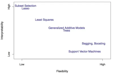
In modelling there is always a trade-off between interpretability and accuracy, well captured in James et al. (2014) (see Figure 1.1). Most of the best predicting techniques are criticized by their lack of interpretability.

(10)

Figure 1.1: A representation of the trade-off between flexibility and interpretability, using different statistical learning methods. In general, as the flexibility of a method increases, its interpretability decreases. (Figure 2.7 and text from James et al. (2014))

In the above image, tree methodology is located halfway between flexibility and interpretability. Boosting is a highly flexible methodology but poorly interpretable. Flexible techniques increase the prediction performance as well, but reducing its interpretability even more.

When using flexible techniques, a major drawback to be avoided is overfitting. Presented in Chapter 3, overfitting represents a problem: when working with training data, an overfitted algo-rithm seems to create very accurate predictions, but it does not predict well when new samples are used.

The outline of this thesis will be the same as the procedure of a datathon, being the principle steps:

1. Identify prediction methods that can be applied to a particular problem and evaluation metrics, Chapter 2.

2. How to create a model that captures the relationship between predictors and outcomes in the training set, Chapter 3.

3. Explanation of the dataset, Chapter 4.

4. Hyperparameter tuning of a XGBoost algorithm, Chapter 5.

(11)

1.2 Supervised Learning

In the field of machine learning there are two main different problems: supervised and unsuper-vised learning. We talk about superunsuper-vised learning when the correct output for your problem is available. For instance, forecasting house prices in a given city based on house features. On the contrary, in unsupervised learning problems the correct outcome is not available. One example could be classifying a company’s costumers in different categories: how many groups will be needed and which traits will differentiate clients belonging to each group is decided during the algorithm implementation.

This thesis will deal with supervised problems, where you have a training set with multiple features. Considering that xij is the value of the jth predictor for the ith data point, where

i= 1. . . n and j = 1. . . m, the objective is to predict the outcome yi.

In this process there are two elements to take into account. First, themodel and parameters

that will perform the predictions for the outcome yi. Second, the metric that allows to measure

how well our model is performing: the objective function. These elements vary depending on the structure of the outcome yi: if it is continuous the problem will be categorized as regression

and if it is discrete as classification.

Model and parameters

The model can be defined as the formula or mathematical rule, or the algorithm, that enables the prediction for the outcome yi. For example, in a generalized linear model yi can be predicted

by means of the proper formula: ˆyi = Pjθjxij for regression problems or ˆyi = τ(Pjθjxij) for

classification problems, being τ(z) = ₁₊1_e−z in the specific case of a logistic model.

For each problem the interpretability of the outcome yi is different and also the estimated

parameters θj. For instance, linear regression models predict a real value while logistic models

predict a probability. There are two different types of parameters θj: the ones that are calculated

directly by the algorithm (in this case, the coefficients of a linear regression) and the ones that the modeller will have to preselect and find the best ones. The second ones are called tuning parameters and will be discussed in Chapter 3.

Objective function

The objective function is the numerical criterion that allows to quantify how well the model is performing. It is divided in two terms: the loss function l(Θ) and the regularization term Ω(Θ):

(12)

Loss function

The loss function evaluates how well the model is predicting when using the current sample. One of the most common loss functions is the mean square error (MSE):

l(θ) = 1 n n X i=1 (yi−yˆi)2.

If a loss function is used without adding a regularization term, complex/flexible models would always perform better than simple/rigid models due to the larger number of parameters, allow-ing for a better adjustment. Two potential problems may arise in this case: unnecessary model complexity and overfitting. To control these problems, the regularization term Ω(Θ) is introduced.

Regularization

The regularization term Ω(Θ) is a penalty for the coefficients of the algorithm that shrinks them to zero in order to avoid capturing the noise of the data. This term is defined differently de-pending on the methodology used because the elements that may overfit your data vary dede-pending on the methodology. The regularization term is applied in the coefficients because an overfitted model is usually characterized by it large coefficients.

For regularization there are two main penalties for the parameters: L1 and L2. L2 was in-troduced in Hoerl and Kennard (1970) for ridge regression. L2 penalizes the objective function through a second-order penalty, Ω(Θ) =λPm

j=1θ2j. The larger is λ, the higher is the shrinkage of

the parameters towards 0. L1 was introduced in Tibshirani (1994) forleast absolute shrinkage and

selection operator, frequently called lasso. In this case, the regularization parameter α is applied to the sum of the absolute value of the model parameters: Ω(Θ) =αPm

j=1|θj|. The absolute value

penalization can set some parameters to 0 and conduct regularization and feature selection at the same time.

According to this modelling process, learning is defined as the minimization of the objective function, in a way that patterns in the data are detected and used to predict new samples.

1.3 Elements of a datathon

A datathon is a particular case of a predicting problem. It is a contest where the participants have limited time to achieve the best predicting algorithm for a given dataset. The main goal of these competitions is to assess the best predictions. There are different kinds of datathons, mainly defined by the nature of the outcome y that must be predicted: regression, classification and recommender systems. The main elements of a datathon are the following:

Data: Two datasets are delivered to participants:

(13)

1.-Train: A train dataset is defined as the one that includes the value of the outcomey along with the matrix x that contains the predictors for each data point. A train dataset includes n rows and m columns for all the data points.

2.-Test: A test dataset contains a matrix x with the same structure as the previous one, but it does not include the value of the outcome y.

Evaluation Metric: The evaluation metric is the numeric criterion that compares the predic-tion for the test dataset ˆyi with the real valuesyi. This comparison is used as the loss function for

the algorithms. By providing a common evaluation metric for all the participants in the datathon, a fair evaluation and ranking of the predictions of the contestants is possible. Some evaluation metrics are introduced in Section 2.3.

Leader board: The leader board is where the results of the evaluation metric are shown. During the competition the results of the leader board are public and are calculated using only the 5%-20% of the test data. This avoids to overfit your predictions with the leader board data. The results are actualized in real time and participants know in any moment how their results are compared with other contestants.

With all these elements in place, the objective is to train an algorithm that captures the rela-tionship structure between predictors and outcomes in your training dataset, without overfitting it.

1.4 Why XGBoost?

Gradient tree boosting was introduced by Friedman (2000) and there are other R implementations such as: (GBM, Ridgeway (2015)). One may thin, what makes Chen et al. (2016) so popular? And why this thesis is focused on XGBoost implementation? There are mainly four reasons:

1. Fast computing: The capacity to do parallel computation in one single machine, as well as the implementation of a sparsity aware algorithm (Section 2.2), makes it 10 times faster than other implementations Chen and Guestrin (2016).

2. Flexible: It can costume objective functions and easily handle missing values.

3. It works: XGBoost allows to run cross-validation in each iteration of the algorithm. It has achieved state-of-the-art results in several data competitions and it is an end to end developed system.

4. Open source: There is a community that improves the algorithm at Distributed (Deep) Ma-chine Learning Community (2017).

(14)

1.5 Notation

The notation used in this thesis homogenizes the two main reference sources that have been em-ployed: Kuhn and Johnson (2013) and Chen and Guestrin (2016).

D={(xi, yi) :i= 1, . . . n},|D|=n, xi ∈Rm, yi ∈R, the training dataset.

n = the number of data points.

m = the number of predictors, also known as features. yi = the ith observed value of the outcome,i= 1. . . n.

ˆ

yi = the predicted outcome of the ith data point, i= 1. . . n.

y = a vector of all n outcome values.

xij = the value of the jth predictor for the ith data point, i= 1. . . n and j = 1. . . m.

xi = a collection (i.e., vector) of the m predictors for the ith data point, i= 1. . . n.

X = a matrix of m predictors for all data points; this matrix has n rows and m columns.

X’ = the transpose of X.

ft(x) =wq(x), w ∈RT, q:Rm → {1,2,· · · , T} = definition of a tree. q = structure of a tree. Maps observations to leafs.

T = number of leafs in a tree. w = leaf weight vector.

k = number of trees.

γ = minimum split loss reduction.

t = the number of iterations of the algorithm. g = first derivative of the loss function. h = second derivative of the loss function.

(15)

L(Θ) = the objective function.

l(Θ) = loss function.

(16)

Chapter 2 Prediction methods

There are a wide variety of prediction methods in the literature. Kuhn and Johnson (2013) group them in three categories: linear models, non linear models and tree based models. Each category includes different algorithms; (1) linear models include Linear Regression, Logistic Regression, Penalized Linear Models and Lasso; (2) nonlinear models include Neural Networks, k-Nearest Neighbours and Support Vector Machines; (3) tree models include Classification and Regression Trees, Bagging, Random Forest and Tree Boosting. There are others models not mentioned and also another classification could be: for parametric and non parametric models.

The scope of this chapter is to review and provide a better understanding of the evolution of tree models. This evolution started with the introduction of CART models by Breiman et al. (1984), followed by Bagging, Random Forest and, nowadays, Tree Boosting. For each one it will be reviewed their history and the objective of their modification; in Chapter 5 it will be shown how this evolution is captured as XGBoost parameters.

2.1 Tree models

Tree models were introduced by Breiman et al. (1984) as Classification and Regression Trees (CART). The aim of tree methods is to create recursive partitions for the predictor space X in order to create homogeneous groups for the outcome y. The goal of the algorithm is to create the most similar groups for the xi observations, based on their yi value. This recursive partitions are

based on thresholds defined on xj values.

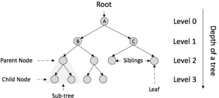
Figure 2.1 helps to understand the tree structure. For the entire dataset in the root of the tree, the first split at the level 0 is the one that generates the most homogeneous groups for the level 1. If the tree stopped there, the prediction of a new observation could be understood as an

if-then statement, explained in Kuhn and Johnson (2013):

If Predictorxjis greater than or equal to threshold then

prediction foryequals to mean ofyfor the training observations in Node B

(17)

else predict the mean ofyfor the training observations in Node C

Figure 2.1: Structure of a tree algorithm.

This recursive partitions could be going on until there is only one observation left or a stop-ping criteria is achieved. Trees have different parts; the final nodes in a tree algorithm are the

leaves. For each leave a different prediction is achieved. The number of partition levels that a tree achieves is the depth of a tree. Two nodes in the same level are called siblings and, as shown in the bottom-left part of Figure 2.1, a tree is constructed by different sub-trees.

As mentioned before, the prediction for a new sample is achieved by following the conditions of the tree until it is assigned to a final leave. Once one observation is in a leave, there are two ways to assign a value: by mean or voting, voting only make sence for classification. For binary classification, if an ending leave has 10 observations, 7 positive and 3 non positive, voting will achieve a positive value while computing the mean will grant a 70% of probability to be a positive observation.

Nowadays trees are a very popular modelling technique for several reason. They are easy to interpret. The threshold splitting is easy to be understood by people who are not into statistical analysis and the splitting order does feature selection. They are easy to implement and compute in parallel, so different machines can calculate different trees or different sub-trees at the same time. Besides trees do not need pre-processing for the predictor form and can easily handle missing data. One of the main disadvantages of models consisting in a single tree model is that they are very unstable. Slight changes in the data could change the partitions order in the tree and achieve a different predictive performance. Also, the recursive partitions splits of the predicting space and subspace are made in rectangles. If the relationship between the features and the outcome y is not this one, this will lead to less optimal performance.

A tree is defined as:

(18)

where w is the leaf weight of a tree, q is the structure of a tree that defines a partition in _Rm

and assign each data point to its leaf and T is the number of leafs. In this growing process a tree algorithm has to determine the following:

1. The predictor to split on and the value of the split. 2. The number of partitions from the root to a leaf.

3. The prediction for an observation. In this case the mean of the node or majority vote. The loss function is different depending on whether the outcome variable is continuous or bi-nary.

Continuous data:

The partition method starts trying for each predictor all the possible splitting values. This is the exact greedy algorithm explained in Algorithm 5. For continuous data the sum of square errors is computed: SSE=Pn

i=1(yi−yˆi)2. Then for a given split,

SSE= X i∈X1 (yi−yˆ1)2+ X i∈X2 (yi−yˆ2)2,

the threshold that achieves the minimum value for SSE is selected. This objective function is adaptable to the modeller criteria. It has to be differentiable of second order. As explained in Section 1.2, a regularization parameter in the objective function is needed to avoid overfitting. For example, the objective function could be penalized by the number of terminal nodes, cp. This

parameter should be estimated by cross-validation.

SSEcp =SSE+cp(T erminalN odes).

Binary data:

For binary data, the objective is the same but the splitting rule is different. In a two-class problem the Gini index for a given node is defined as:

p1(1−p1) +p2(1−p2).

This is summarized by 2p1p2. The minimization of this index is creating pure nodes, where p1 or p2 are close to zero. When the node has p1 = p2 achieves its greatest value. The splits are searched using the Algorithm 5 and evaluates all possible values until finds the one that minimize the Gini index after split. This maximization is recursive until a stopping criteria is found: minimum samples in a node or maximum depth of a tree. For further information, Kuhn and Johnson (2013) Section 14.1.

(19)

2.1.1 Bagging

Bagging was one of the first ensemble techniques presented in Breiman (1996). Ensemble is to use more than one model and combine their predictions. In this particular case several tree models are combined. Bagging stands for bootstrap aggregation. Bootstrap is a resampling technique with replacement introduced by Efron that is explained in detail in Efron and Tibshirani (1993). This resampled new training data has to be as large as the training set. The algorithm is as follows:

Algorithm 1 Bagging. (Extracted from section 8.4 at Kuhn and Johnson (2013).)

for i = 1 to T do

Generate a bootstrap sample of the original data Train an unpruned tree model on this sample

end

Given a structure of a tree, an ensemble method for predicting new observationxi can be the

average of the scores.

One of the main advantages of bagging models is that they provide an internal estimate of pre-dictive performance. This estimate is obtained thanks to how resample is done: when bootstrap resample is done as big as the training set, some observations are not used. These are called out of the bag (OOB) observations. They can be used to assess the performance of the model since they are not used in the construction of the model. In some way these estimated performance could be understood as an internal cross-validation. In addition, this aggregation process reduces the variance of the predictors.

The trade-off of a bagged model is that their output is less interpretable and the generated trees are highly correlated, due to their similar structure. Could not seem very logical to average correlated predictors to reduce the training variance.

2.1.2 Random Forest

Since the bagging tree introduces a random component in the sample generation, the generated trees are not mutually independent. They are not because the predicting variables available used to construct each tree are always the same, no matter which tree is built. Most of the trees will have the same structure, essentially in the top of the nodes. This is known as tree correlation.

To reduce this correlation among predictors, in addition to include randomness in the obser-vations, randomness in the predictors can also be included. The generalization of this algorithm was introduced in Breiman (2001) and is known as Random Forest. The idea is the following: the algorithm selects random predictors at each split, reducing the tree correlation. The number of candidate random predictors at each split m acts as a tuning parameter of the algorithm. The

(20)

algorithm is as follows:

Algorithm 2 Basic Random Forests. (Extracted from section 8.5 at Kuhn and Johnson (2013).) Select the number of models to build, t

for i = 1 to T do

Generate a bootstrap sample of the original data Train a tree model on this sample

for each split do

Randomly select mtry(< m) of the original predictors

Select the best predictor among the k predictors and do a partition of the data

end

Use typical tree model stopping criteria to determine when a tree is complete (but do not prune)

end

As the Bagging algorithm (mentioned above), Random Forest is an ensemble algorithm that uses bootstrap resampling. Due the randomness in observations and predictors, trees could be considered independent to each other. By averaging the different trees predictions, you get ride of tree high variance. Also as a resample technique on of the main advantage is the usage of the out of the bag observations. These observations are used to calculate error estimates. Random Forest also assess variable selection, achieves a better performance than bagging models and reduces the risk of overfitting due to the independent trees. However, Random Forest is also hard to interpret.

2.1.3 Tree Boosting

Boosting theory was develop by Valiant (1984); the main idea behind this algorithm is that many weak classifiers, better than a random guessing, could create a strong classifier when used in com-bination. Boosting was first implemented in the Adaboost algorithm Freund and Schapire (1996), but Friedman (2000) connected the concepts with Statistics and stablished the boosting framework. Boosting is astage-wise additive modelling. Starts without a classifier and a first weak classi-fier is fit to the data. Another weak classiclassi-fier is fitted to improve the current model performance, without changing the past classifiers and so on. This new classifier has to take into account where the pasts classifiers are not performing well. Given the previous classifiers, the next classifier is the one that decreases the most the objective function.

(21)

Algorithm 3 Forward Stagewise Additive Modelling. (Extracted from section 10.2 at Hastie et al. (2001).) 1. Initialize f0(x) = 0. 2. For t= 1 to T: (a) Compute (βt, ζt) = arg min β,ζ N X i=1 l(yi, ft−1(xi) +βb(xi;ζ)). (b) Setft(x) =ft−1(x) +βtb(x;ζt)

In general terms boosting could be understood as: given a loss function, a response variable and a current model, at each state t figure out the best improvement to the current model with another classifier and update the model with this classifier. This update can be regularized before it is added.

Boosting could be applied to several statistical techniques, so why it should be used to trees? A shallow tree could be considered a weak classifier. Also, trees are very flexible: they can be generated very quickly, have different parameters to be tuned and the result of a tree can be added with the results of other trees.

The main difference between boosting and random forest is how the ensemble procedure is done. In Random Forest the trees are independent, can reach their maximum depth and con-tribute equally. In boosting it is quite different: trees depend on past trees, have limited depth and contribute differently to the final model.

In order to avoid overfitting, the learning process of boosting could be shrink by applying a reg-ularization term η. They are parameters of the XGBoost model and are detailed in Section 5.1.1. The methodology is explained following Chen and Guestrin (2016) and Distributed (Deep) Ma-chine Learning Community (2016).

An objective function is needed to start training a tree boosting algorithm. As defined in Section 1.2 this function contains two parts, the loss function and the regularization term:

L= n X i=1 l(yi,yˆ (t) i ) + K X k=1 Ω(fk).

This following methodology could seem a bit confusing at first sight because it is the generalization to any objective function with first and second order derivatives.

(22)

Model training:

The sequential training is performed in an additive manner: given what was learned in the tree fi, add a new tree at a time. For each step t the outcome is

ˆ y_i(0) = 0 ˆ y_i(1) =f1(xi) = ˆy (0) i +f1(xi) ˆ y_i(2) =f1(xi) +f2(xi) = ˆy (1) i +f2(xi) . . . ˆ y_i(t) = t X k=1 fk(xi) = ˆy (t−1) i +ft(xi)

Substituting the ˆy_i(t) in the objective function:

L(t)= n X i=1 l(yi,yˆi(t)) + t X i=1 Ω(fi) = n X i=1 l(yi,yˆ (t−1) i +ft(xi)) + Ω(ft) +constant

For each iteration, the ft tree that most improves the objective function is added. Using the

MSE as the loss metric and removing constant terms:

L(t)= n X i=1 (yi−(ˆy (t−1) i +ft(xi)))2+ Ω(ft) +constant = n X i=1 [2(ˆy(_it−1)−yi)ft(xi) +ft(xi)2] + Ω(ft) +constant

To improve the optimization, the loss function is approximated by the second order Taylor expansion: L(t)≈ n X i=1 [l(yi,yˆ (t−1) i ) +gift(xi) + 1 2hif 2 t(xi)] + Ω(ft) +constant Where, gi =∂_y_ˆ(t−1) i l(yi,yˆ (t−1) i ), and hi =∂_y2_ˆ(t−1) i l(yi,yˆ (t−1) i ),

(23)

are respectively the first and the second order derivatives of the loss function. Removing all the constants, the specific objective function at step t is,

L(t) ≈ n X i=1 [gift(xi) + 1 2hif 2 t(xi)] + Ω(ft).

being the new optimization goal for the new tree. As an example in terms of square loss:

gi =∂_y_ˆ(t−1) i (yi−yˆ (t−1) i ) 2 _{= 2(ˆ}_y(t−1) i −yi) hi =∂_y2_ˆ(t−1) i (yi−yˆ( t−1) i ) 2 = 2.

Using the square loss as the loss function without a regularization term in boosting algorithm is equal to retrain the model with the previous predicting errors. The new tree is the one that best improves the past predicting errors. XGBoost is a framework where users can predefine their own objectives functions that have first and second order derivatives, avoiding to use predefined functions. Now let’s figure it out how to find the best tree in iteration t.

Model complexity:

Once the training steps are introduced, the regularization term of this training steps is intro-duced: Ω(f) =γT +1 2λ T X j=1 w2_j.

T is the number of leafs, γ is the minimum split loss reduction, λ is the regularization term on the weights and wj are the weights of each leaf. There are multiple definitions of the

regulariza-tion term but this is the default set up in Chen et al. (2016). Considering that Ij = i|q(xi) =j,

expanding Ω and replacing ft(xi) by the tree definition wq(xi):

L(t) ≈ n X i=1 [giwq(xi)+ 1 2hiw 2 q(xi)] +γT + 1 2λ T X j=1 w2_j = T X j=1 [(X i∈Ij gi)wj + 1 2( X i∈Ij hi+λ)wj2] +γT.

The optimal weight for w_j∗ on a leafj can be computed: w∗ =−

P

i∈Ijgi

(24)

So, the tree with the best weights is:

L∗ =−1 2 T X j=1 (P i∈Ijgi) 2 P i∈Ijhi+λ +γT.

This expression is used as the scoring function for a tree structure. It is the same as the impurity score of a decision tree but allows for evaluating wider objective functions. Given a function to evaluate a tree structure in the iteration t, the next step is to find the best tree to ensemble to the past trees. This procedure is done by growing a new tree in a greedy way (Algorithm 5), this tree has the best gain in their splits:

Gain= 1 2 ñ (P i∈ILgi) 2 P i∈ILhi+λ + ( P i∈IRgi) 2 P i∈IRhi+λ − ( P i∈Igi)2 P i∈Ihi+λ ô −γ.

Gain function could be decomposed as follows: the score of the left leaf, the score of the right leaf, the score of the original leaf and the regularization term. If the gain is smaller than the regularization term, do not add that branch. The tree score function it is used in every step, so the exact greedy algorithm selects the split that increase the most the gain function. For each iteration t the next tree is grown following this greedy criterion in order to minimize the loss function with the gradient statistics in this moment.

Before ending with this section, another example it is introduced to understand better boost-ing methodology. If the loss function is the squared error and the boostboost-ing tree is trained for regression, it can be understood as:

Algorithm 4 Simple Gradient Boosting for Regression. (Extracted from section 8.6 at Kuhn and Johnson (2013).)

Select tree depth, P and number of iterations, B.

Compute the average response, and use this as the initial predicted value for each sample.

for b = 1 to B do

Compute the residual, the difference between the observed value and the current predicted value, for each sample.

Fit a regression tree of depth, P, using the residuals as the response. Predict each sample using the regression tree fitted in the previous step.

Update the predicted value of each sample by adding the previous iteration’s predicted value to the predicted value generated in the previous step.

end

2.2 Split finding algorithms

Once the splitting function is defined, the split in the dataset must be chosen. As we saw before Section 2.1, one option is to evaluate all the possible splits of our features. This is called exact

(25)

greedy algorithm. The algorithm sorts the feature and accumulates the gradient statistic for each point. As you can imagine, this process is very computationally demanding.

Exact greedy algorithm

Algorithm 5 Exact Greedy Algorithm for Split Finding. (Extracted from section 3.1 at Chen and Guestrin (2016).)

Input: I, instance set of current node

Input: d, feature dimension gain ←0 G←P i∈Igi, H ←Pi∈Ihi for k = 1 to m do GL ←0,HL ←0 for j in sorted(I, by xjk) do GL ←GL + gj, HL ←HL +hj GR ←G−GL, HR ←H−HL

score ←max(score, G2L

HL+λ + G2 R HR+λ − (GL+GR)2 HL+HR+λ) end end

Output: Split with max score

The exact greedy algorithm is not feasible if all the data cannot be stored in memory, and also in distributed setting. There are some approximations based on having some prior candidates of splitting points, in this case the percentiles.

Approximate Algorithm

Algorithm 6 Approximate Algorithm for Split Finding. (Extracted from section 3.2 at Chen and Guestrin (2016).)

for k = 1 to m do

Propose Sk ={sk1, sk2, . . . skl} by percentiles on the feature k.

Proposal can be done per tree (global), or per split (local).

end

for k= 1 to m do

Gkv ←Pj∈{j|sk,v≥xjk>sk,v−1}gj

Hkv ←Pj∈{j|sk,v≥xjk>sk,v−1}hj

end

(26)

The procedure is as follows. The algorithm proposes candidate splitting points, based on per-centiles of the feature distribution. Then it maps the feature into buckets and aggregates the statistics to find the best split.

The algorithm has two variants: the global variant and the local variant. The global variant proposes all the splits before the splitting phase and uses the same proposed split in the next levels. The local variant proposes the split after. As is shown in Chen and Guestrin (2016), the global proposal can be as good as the local one if enough candidates are available. In XGBoost the number of candidates for this approximation is controlled by means of a parameter (sketch eps) defined in Section 5.1.1.

Sparsity aware

In a lot of real problems, the matrixXis very sparse, that means that most of its elements are zero. Sparsity can be due to a several factors: presence of missing values, zero entries in a feature because is encoded as a dummy variable or the nature of the variable. In order to select the splits, it is important to make the algorithm aware of this sparsity. To avoid this problem, the algorithm has a default classification direction (a default path in the tree) for the observations with missing values. This direction is learned from the data following the next steps.

(27)

Algorithm 7 Exact Greedy Algorithm for Split Finding. (Extracted from section 3.4 at Chen and Guestrin (2016).)

Input: I, instance set of current node

Input: Ik={i∈I|xik 6= missing}

Input: d, feature dimension

Also applies to the approximate setting, onlye collect statistics of non-missing entries into buckets gain ←0

G←P

i∈Igi, H ←Pi∈Ihi

for k = 1 to m do

// enumerate missing value goto right GL ←0,HL ←0

for j in sorted(I, ascent order by xjk) do

GL ←GL + gj, HL ←HL +hj

GR ←G−GL, HR ←H−HL

HL+λ + G2 R HR+λ − (GL+GR)2 HL+HR+λ) end

// enumerate missing value goto left GL ←0,HL ←0

for j in sorted(I, ascent order by xjk) do

GL ←GL + gj, HL ←HL +hj

GR ←G−GL, HR ←H−HL

HL+λ + G2 R HR+λ − (GL+GR)2 HL+HR+λ) end end

Output: Split and default directions with max gain

This algorithm treats the non-presence as missing values, and learns the best direction to be assigned. So the algorithm predefines the default node direction if the feature that must be predicted in the split is missing. This is also suitable for specific values that the modeller wants to treat as missing. As shown in Chen and Guestrin (2016) the sparsity algorithm makes the computation nearly 50 times faster.

2.3 Evaluation metrics

There are different performance metrics to evaluate the prediction model outcome. Each met-ric has its nuance, but all of them share a common objective: evaluating the effectivity of the model. Two of the most common evaluation metrics for predicting will be presented as follows: the root mean square error (RMSE) for regression problems and the receiver operating charac-teristic (ROC) curve and the area under this curve, for classification problems. As mentioned in Kuhn and Johnson (2013) the evaluation of the strength or weakness of a model cannot rely solely

(28)

in a singular evaluation metric.

Root Mean Square Error (RMSE)

This is the most popular method when the outcome is numeric. The RMSE represents the sample standard deviation of the differences between predicted values and observed values. The square root operator ensures that the measure has the same units as the original data:

RM SE = Ã 1 n n X i=1 (yi−yˆi)2.

Area Under the Curve (AUC)

The area under the curve is one of the most commonly used evaluation metrics for data compe-titions, when the response variable is binary. The referred area is drawn by the receiver operating characteristic (ROC) curve. The idea of the curve is to evaluate different class probabilities for all the possible thresholds.

When a binary classifier is evaluated, the model predicts the different class probabilities. For instance, for a given sample the probability of being a positive observation could be 20% and for another one 70%, also this could be referred asscore. These probabilities has to be converted into binary classifiers so you can check the accuracy of your model. The matrix where the predictions and the observations are cross is the confusion matrix.

To not manually check which is the best threshold for our model, the ROC curve evaluates all the possible cut-off and creates a curve for the predictability of our model. The area of this curve is defined from 0 to 1, being 0 the worst classifier and one a perfect classifier. Also a random model will achieve a 0.5.

It can be proved that the AUC coincides with the probability that the score of a negative obser-vation is bigger than a positive obserobser-vation. See Altman and Bland (1994) for further information.

(29)

Data splitting and Parameter tuning

Once the methodology has been detailed, let’s focus on how to create a model that captures the relationship between predictors and outcomes in the training set in order to make good predictions for new samples. As such models are highly flexible, they could capture the noise and not the representative patterns. Two different aspects must be taken into account to successfully use this model: the parameters of the algorithm and thedata used to train.

Some parameters of the algorithm cannot be adjusted numerically in order to find their best possible value, so they have to be tuned (see Section 3.2). Regarding the available data, the idea is to find a way to make predictions in a set not used for training. This set, called validation set or hold out sample, allows to approximate how well the model is performing and it is tested by cross validation (Section 3.3).

All this efforts are made to avoid overfitting (Section 3.1). Overfitting is the worst enemy we face when using a modelling technique, because it makes us believe that our predictability power is very high when in fact it is not. This chapter is inspired by Kuhn and Johnson (2013), Chapter 4.

3.1 Overfitting

Overfitting occurs when a model captures patterns that are not reproducible. If the evaluation metrics in the training set are lower than expected, it is easy to conclude that the model is per-forming well. However, this is not true in most of the cases; it is more likely that the model has learned not only the structure of the data but the noise of the sample as well. When a model learns the noise of the data, generalization of the model to new samples is not possible (or it is not good enough).

There are some tools that may help to prevent our model to overfit. The regularization term in the objective function and the resampling techniques are good examples. The evolution of tree algorithms are based in this two techniques, as mentioned in Chapter 2. The step needed to go from CART to Bagging/Random Forest implies adopting resampling techniques for observations

(30)

and columns One of the biggest improvements provided by the XGBoost implementation over GBM was due to the introduction of a regularization term Ω(Θ).

Modern algorithms are currently evolving in a way that they are able to avoid overfitting. For instance, Boosting techniques iteratively build trees based on the prediction error of previous trees, in such a way that avoiding overfitting is much more difficult than in non Boosting techniques. For that reason, establishing a methodology to approach model evaluation is a critical success factor.

3.2 Model tuning

There are different model parameters that cannot be optimized analytically, they have to be op-timized numerically. The selection of values for these parameters is done by testing a wide range of candidate values; this procedure is called model tuning.

A good example of this procedure is how k-Nearest Neighbours (k-NN) algorithm is tuned. As explained in Cover and Hart (1967), k-NN predicts the value for the testing data based on the k-nearest observations in an Euclidean space. There is no analytical formula to calculate the optimal value of k for the sample, rather than tuning the parameter, numerical approach. That is, trying different possible values for k. One can imagine that a small value of k could have a low predictive power and a high one could overfit the data.

As a practical guide, parameter tuning could be stipulated as the following steps, Kuhn and Johnson (2013):

1. Define a set of parameter tuning candidates. 2. For each candidate.

(a) Resample data or split the dataset. (b) Fit a model.

(c) Predict the hold out. 3. Aggregate the performance.

4. Determine the best tuning parameters. 5. Train with all model.

The idea is very simple: evaluate your model in samples that are not used for training, as it has been explained before for the validation of the out of the bag samples for random forest. Another important consideration when splitting the data is to maintain the same proportion of the outcome y in every split, and also in a second level, to have the same correlation with the features.

(31)

3.3 k-fold cross validation

K-fold cross validation is the most commonly used technique for model training. The idea is to create a k-equal size split for the dataset, train a model usingk−1 splits and predict the outcome for the remaining split. As an example, imagine that the training dataset is partitioned in 10 folds, the model is trained using the first 9 folds and prediction is done using the 10th fold. In the next iteration, the training is done using all the folds except the 9th and later prediction is one using this one, and so on.

Given a set of parameters to tune, after k iterations, k evaluation metrics are calculated. In each iteration, prediction is done in the hold out sample and the k evaluations metrics calculated can be summarized by its mean value and standard deviation. Later on, the model is trained using the hole training set and the best tuning parameters. This is a more robust estimate of how your tuning parameters are working in this model.

K-fold is quick to compute, has a low bias and an acceptable variance. Nowadays this procedure is implemented in several R packages; Caret (Kuhn (2016)), MLR (Bischl et al. (2016)). Coding this procedure requires no more than 10 lines of code. Following an example of a procedure for tuning a Random Forest is shown:

library(caret) model <- train( (1) data = training_data, (2) method = "ranger", (3) outcome ~. , (4) tuneLength = 10,

(5) trControl = trainControl(method = "cv", number = 5))

The previous lines of code could be interpreted as the following steps; (1) train a model in the training data dataset. (2) Use therangerfunction (fromranger package Wright (2016), Random Forest algorithm). (3) Use all the variable available to predict the outcome and (4) select for the tuning parameter 10 possible values. The last line of code (5) executes the procedure using cross validation and setting the number of folds to five.

(32)

Chapter 4 Data and description

In this chapter is going to be illustrated what it is explained in previous chapters with a real dataset. The dataset used is part of the first Datathon that took place in Barcelona in the weekend of November 14th, 2015, BCNAnalytics (2015). The objective is to predict which users will stop playing an online videogame, also called churn. This is a very important metric in the videogame industry. The videogames are free to play, but the users that keep playing are more likely to pay. The users pay to increase their level, get special items and other stuff depending on the game. The game is Dragon City SocialPoint (2016); the purpose of the game is to collect all the dragons that are available, train them and combat with other player’s dragons.

4.1 Descriptive

The following variables were the available in the dataset, and described as the competition docu-mentation:

• register ip country: the two-digit country code of the user.

• num sessions: number of times that the user opened and played the game within the first 48 hours after registration.

• churn: 1 if the user churned out of the game within 7 days of registration, or 0 if the user was still playing after this time.

• max level reached: game level that the user obtained in the first 48 hours.

• reach level 3: 1 if the user passed through the tutorial and 0 if the user left the game before finishing the tutorial.

• cash spent: total number of gems (in-game currency) that the user spent within the first 48 hours.

• spents: number of times the user spent gems (in the first 48 hours).

• dragons lvl up: number of dragons that the user has levelled up. 27

(33)

• lvls up: number of times that a user has fed their dragon to the next level.

• breedings: number of times that a user has bred a dragon (within the first 48 hours).

• facebook connected: the game allows users to connect to Facebook so that they can share their progress with their friends, and so that their friends can help them to progress in the game. This variable is 1 if the user has connected to Facebook in the first 48 hours, 0 otherwise.

• number goals: the game suggests a number of things that the users can do to progress, these are called goals and this variable tells you how many goals were accomplished during the first 48 hours.

• played day 2: is a 1/0 variable that tells you if the user played on the second day as well as the first.

• attacks: users can battle their dragons in the game, this variable tells you how many battles the user did in the first 48 hours.

• attacks wins: number of battles that the user won in the first 48 hours.

• last cash: how many gems the user had at the end of 48 hours.

• last gold: the amount of gold the user had at the end of 48 hours.

• last food: the amount of food the user had at the end of 48 hours.

• dragons bought: number of dragons the user acquired by spending gems in the first 48 hours.

• num sessions 1d: number of times the user opened the game on the 1st day.

• num sessions 2d: number of times the user opened the game on the 2nd day.

4.2 Feature Engineering

Feature Engineering is a procedure to create new features for the algorithm. The goal of this pro-cedure is to help the algorithm to achieve better results. These results are obtained by optimizing the objective function and delivering better predictions. The idea behind feature engineering is to provide new dimensions to the algorithm where it can learn better. From a more general perspec-tive, feature engineering can be seen as a transformation of the data to achieve a better description of the problem resulting in a better model prediction.

One example of feature engineering in a classification problem is adding a new dimension where the positive and negative samples can be easily separated by the algorithm. In tree algo-rithm a feature that is working properly for prediction purposes may be selected in the firsts splits.

(34)

The most basic feature engineering procedure is the nowadays called one hot encoding, or dummy variables. One hot encoding method is to binaries a multifactor variable. An example is, given a weekday, to create new binary feature if is this weekday. Other way to create features is using the components of a Principal Component Analysis (PCA). Creating features with a di-mensional reduction technique is called feature extraction.

While you use feature engineering, you have to take into account the learning procedure of your algorithm. Trees have problems with splitting data when the class boundary is diagonal, because trees split data in a linear way. The features that you create must be related to the capacity of the algorithm you train to learn them.

There is not a single procedure for feature engineering; in fact, some modellers consider it an art. When you create the features for your problem you do not know if they are going to work. In order to estimate to what extent the features are useful an univariate descriptive analysis with the outcome can be used, such as the Pearson correlation, but is not a 100% reliable rule. Feature engineering is the key for a successful algorithm implementation.

(35)

Hands on XGBoost

Setting up a XGBoost model it is easy, but improving the model it is much more difficult. The difficulty is caused by what makes it so powerful: the flexibility. This flexibility helps XGBoost to perform extremely well with different data types and be one of the best algorithms for data science. The cost of this flexibility is the need of setting up more than twenty parameters. The correct set up for this parameters is unknown in advance and could not be learned from the data. As mentioned in Chapter 3, parameter tuning must be done by cross validation. The permu-tation of all the possible values for all the parameters to be tuned could produce an extremely large number of different scenarios. In this chapter the most important parameters in XGBoost for parameter tuning will be reviewed, as well as the way to tune them.

5.1 Parameters

This is a summary of what can be found at Distributed (Deep) Machine Learning Community (2017). The authors define three different groups of parameters for XGBoost set up:

1. General parameters: Parameters to configure the overall algorithm, such as booster type, printed messages and parallel processing.

2. Parameters for Tree Booster: Parameters to configure the booster. Only tree booster parameters will be reviewed because they outperform the linear ones.

3. Learning Task Parameters: Parameters related to the objective function and the evalu-ation metric.

In this Section only tree booster parameters and learning task parameters will be explained, due to the relevance of their tuning process to produce better predictions.

To have a clear idea before going into details, a XGBoost parameter configuration will look like this:

(36)

param <- list("objective" = "binary:logistic","eval_metric" = "auc","max_depth"=5, "eta"=0.2, "subsample"=0.9,"colsample_bytree"=0.5,"prediction"=TRUE, "num_parallel_tree"=5)

5.1.1 Parameters for Tree Booster

This is a summary of the most important parameters for tree learners that must be tuned:

• eta (η): learning rate of the algorithm.

– After each boosting step, the eta shrinks the feature weights to make the boosting more conservative. Range: [0,1]. Default value: 0.3.

• gamma (γ): minimum split loss reduction.

– It is the minimum loss reduction to make another partition on a leaf node. For bigger values the algorithm will be more conservative. Range: [0,inf]. Default value: 0.

• max depth: maximum depth of a tree.

– A lower value prevent overfitting. Higher value could learn relationships specific to the training data. Range: [0,inf]. Default value: 6.

• min child weight (hi): proxy of minimum observation for a child.

– It is the minimum sum required of the Hessian. If the sum is less than the parameter, there will not be further partitioning. Range: [0,inf]. Default value: 1.

• subsample: ratio of random samples to be used for training.

– Equivalent of the percentage of random observations collected to grow each tree. Pre-vents overfitting. Range: [0,1]. Default value: 1.

• colsample bytree: ratio of columns used to train each tree.

– Equivalent of the percentage of random columns collected to grow trees. Range: (0,1]. Default value: 1.

• colsample bylevel: ratio of columns used to train each split of a tree.

– Same as before, but the randomization of columns are for each split. Same as Random Forest. Range: (0,1]. Default value: 1.

• lambda (λ): regularization term on the weights.

– L2 regularization term for the weights. Increasing this value will increase the regular-ization parameter. Default value: 1.

• alpha (α): regularization term on the weights.

(37)

– L1 regularization term for the weights. Increasing this value will increase the regular-ization parameter. Default value: 0.

• tree method: construction tree algorithm.

– Different split finding algorithms for tree constructing. ‘auto’ options leverage ex-act greedy option and approximation depending on the size of the dataset. Choices: ‘auto’,‘exact’,‘approx’. Default value: ‘auto’.

• sketch eps: number of candidates for approximate greedy algorithm.

– This parameter select the number of candidates per feature to be evaluated in each split. This can be translated as 1/sketch eps. Lower values will propose more candidates and be more accurate. Range: (0,1). Default value: 0.03.

• max delta step and scale pos weight: useful for classes extremely unbalanced.

All the parameters could be found in the package documentation.

5.1.2 Learning Task Parameters

For the learning task parameters there is also a great variety. There are two main parameters with several options: the objective function and the evaluation metric. For the objective function only the most commonly used will be described; for the evaluation metric, the ones defined in this thesis.

• objective (_L): definition of the objective function.

– ‘reg:linear’: linear regression.

– ‘reg:logistic’: logistic regression.

– ‘binary:logistic’: logistic regression for binary classification, output probability.

• eval metric (e(Θ)): evaluation metric for the validation data.

– ‘rmse’: root mean square error.

– ‘auc’: area under the curve.

(38)

5.2 Training & Parameter tuning

Tuning the parameters of an algorithm does not follow a stablished methodology. The two elements to take into account are (1) the possible parameters for the algorithm and (2) their performance. As mentioned in Section 3.2, different parametrization of the algorithm must be tested to find their best values in the training set, while avoiding overfitting. To test the different parameter values of the algorithm grid search or random search can be used.

Grid search consists in creating a grid of all the possible/reasonable parameter values for the algorithm. Each row of the grid is a different set up of the parameters and the total of rows is the permutations of all the possible parameter values. Of course, for continuous parameters there is not a way to test all the possible values, but instead either the possible/logical values or their quantiles can be tested. The primary problem of grid search is its computational cost. As an exhibit, the model trained in the Appendix A took 14 hours in a 8 GB RAM computer. Random search, as can be inferred, consists in selecting the different parameter values randomly and testing its results. XGBoost package does not have any hyperparameter tuning options; to do this parametric search caretpackage will be used (the proper code can be found at Appendix B). As a guidance, some modellers use this steps to make parameter tuning for XGBoost:

1. Select a low learning rate η= 0.1

2. Optimize the parameters of the tree booster:

(a) max depth

(b) colsample bytree

(c) subsample

3. Aggregate the performance.

4. Tune the regularization parameters, α and λ. 5. Test lower values for η.

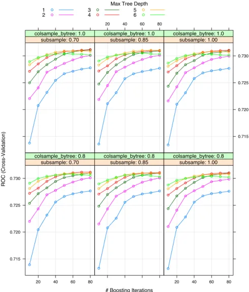
In the first set of parameters the learning parameter η will be fixed at 0.1 and the tuning parameters will bemax depth,colsample bytreeandsubsample. The scope of this first approach is to find the more optimal values for our weak learner. As explained in Section 3.3 the results of this calculus will be done by the aggregation of the AUC metric in the hold out set in k-fold for a cross validation equal to 5.

(39)

# Boosting Iterations ROC (Cross-Validation) 0.715 0.720 0.725 0.730 20 40 60 80 subsample: 0.70 colsample_bytree: 0.8 subsample: 0.85 colsample_bytree: 0.8 20 40 60 80 subsample: 1.00 colsample_bytree: 0.8 subsample: 0.70 colsample_bytree: 1.0 20 40 60 80 subsample: 0.85 colsample_bytree: 1.0 0.715 0.720 0.725 0.730 subsample: 1.00 colsample_bytree: 1.0 Max Tree Depth

1

2 34 56

Figure 5.1: First approach for tuning the parameters of the XGBoost.

According to the previous graph, it is not very clear which is the best number of iterations for the algorithm and the best value for max depth and subsample. The procedure is repeated by dismissing some trees depth values and colsample bytree. Let’s retrain the model with the values that achieved the best performance and with a higher number of iterations.

(40)

Tree Boosting Data Competitions with XGBoost # Boosting Iterations ROC (Cross-Validation) 0.726 0.728 0.730 80 90 100 110 120 130 140 subsample: 0.6 80 90 100 110 120 130 140 subsample: 0.7 Max Tree Depth

4

5 67 8

Figure 5.2: Second iteration for optimal tree depth and subsample.

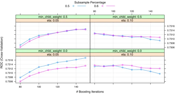
The depth of the tree is finally set up to four; the tree is retrained again using a regularization parameter min child weight and a lower value for the learning parameter eta.

# Boosting Iterations ROC (Cross-Validation) 0.7306 0.7308 0.7310 0.7312 0.7314 0.7316 80 100 120 140 eta: 0.05 min_child_weight: 0.0 eta: 0.10 min_child_weight: 0.0 eta: 0.05 min_child_weight: 0.5 80 100 120 140 0.7306 0.7308 0.7310 0.7312 0.7314 0.7316 eta: 0.10 min_child_weight: 0.5 Subsample Percentage 0.5 0.6

Figure 5.3: Third iteration for learning rate and regularization parameters.

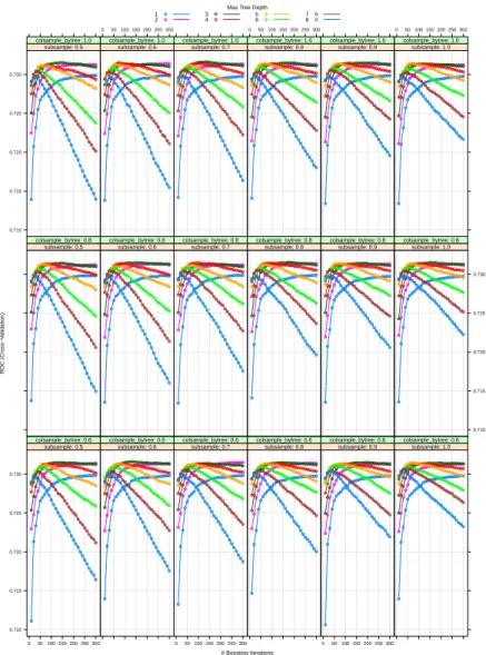
According to the previous graph and other analysis of the performance of boosting for differ-ent values of the ”number of iterations” parameter (detailed in the Appendix A) the number of iterations is set up to 170. Therefore the final parameters of the algorithm are: 170 iterations,

(41)

eta= 0.05,max depth= 4 ,min child weight= 0,subsample= 0.5 andcolsample bytree= 1. The remaining parameters are set up to their default values.

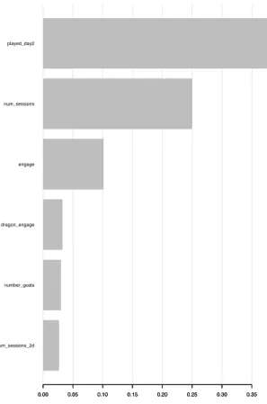
Once the model is trained the xgb.plot.importance() function ranks feature importance based on the usage of each feature in the splits. This also gives insights into the most predicting variables for this problem.

num_sessions_2d number_goals dragon_engage engage num_sessions played_day2 0.00 0.05 0.10 0.15 0.20 0.25 0.30 0.35 0.00 0.05 0.10 0.15 0.20 0.25 0.30 0.35

Figure 5.4: Top 6 more predicting variables.

The most predicting features are: if the player played second day, the total number of sessions, engage variable created by the sum of their achievements (see Appendix B), dragon engage all the engage that is related to the dragon (see Appendix B), the number of goals achieved and the number of sessions of the second day. These features are measured in their % of predictive power against the other features.

(42)

Chapter 6 Conclusions and further research

The main objective of this Thesis has been to provide understanding on how to approach a su-pervised learning predictive problem and illustrate it using the tree boosting methodology. To achieve this goal, an explanation of a supervised problem has been provided as well as a review of the different tree methods developed since this methodology was first introduced in Breiman et al. (1984). Reviewing the tree methodology evolution helps to understand the current tuning parameters techniques.

Tree boosting and the XGBoost implementation is the current state-of-the-art predicting method for numerous problems; a clear signal of its effectiveness it the fact that is the most used algorithm for datathon competitions Chen and Guestrin (2016). Under the scope of compe-titions, algorithms need to take into account deep learning LeCun et al. (2015), when the features are text or images.

To improve the model performance, different possibilities must be taken into account: stack-ing, using XGBoost as a metalearner or dropping some trees. Stacking is an ensemble of different models predictions, for instance, using the predictions of different models as features for a new model. Someone could thing about using logistic regression or the probability of a k-NN as fea-tures. Also in this level of features an XGBoost could be retrained as a metalearner. For this purpose, the training features should be other models’ predictions and maybe some normal fea-tures. Finally, another possibility to improve performance is reducing the number of trees used for predicting. To achieve it; DART (Dropouts meet Multiple Additive Regression Trees, Rashmi and Gilad-Bachrach (2015)) could be used to achieve this goal. Reducing the number of trees is a new technique for tree boosting and has to be explored in greater depth. For instance, a different solution could be running a lasso regression for all the trees in order to preselect the ones more useful for the prediction.

A way to improve the tuning parameter process, could consist on numerical optimization of the evaluation metric (computed by k-fold cross validation) as a function of these parameters. The optimization procedure of choice could be Nelder-Mead method, because it does not need derivative of the objective function.

(43)

Finally, when we seek better performance metrics, an important aspect to be considered is which is the trade-off between better performance metrics and computation/human cost. Training these models takes a lot of time and, sometimes, the gains are not that higher in terms of the evaluation metric. Of course, these gains are key to win a data competition but things are a bit different in real-world predicting problems.

(44)

Bibliography

Altman, D. G. and Bland, J. M. (1994). Statistics notes: Diagnostic tests 3: receiver operating characteristic plots. BMJ, 309(6948):188.

BCNAnalytics (2015). Barcelona gaming data hackathon, http://bcnanalytics.com/hackathon/. Bischl, B., Lang, M., Kotthoff, L., Schiffner, J., Richter, J., Jones, Z., and Casalicchio, G. (2016).

mlr: Machine Learning in R. R package version 2.9.

Breiman, L. (1996). Bagging predictors. Machine Learning, 24(2):123–140. Breiman, L. (2001). Random forests. Machine Learning, 45(1):5–32.

Breiman, L., H. Friedman, J., A. Olshen, R., and J. Stone, C. (1984). Classification and Regression Trees. Chapman Hall, New York.

Chen, T. and Guestrin, C. (2016). XGBoost: A scalable tree boosting system. CoRR, abs/1603.02754.

Chen, T., He, T., and Benesty, M. (2016). XGBoost: Extreme Gradient Boosting. R package version 0.4-3.

Cover, T. and Hart, P. (1967). Nearest neighbor pattern classification. IEEE Transactions on Information Theory, 13:21– 27.

Distributed (Deep) Machine Learning Community (2016). Scalable and flexible gradient boosting, https://xgboost.readthedocs.io/.

Distributed (Deep) Machine Learning Community (2017). Scalable, portable and distributed gradient boosting library, https://github.com/dmlc/xgboost.

Efron, B. and Tibshirani, R. J. (1993). An introduction to the bootstrap. Mono. Stat. Appl. Probab. Chapman and Hall, London.

Freund, Y. and Schapire, R. E. (1996). Experiments with a new boosting algorithm.

Friedman, J. H. (2000). Greedy function approximation: A gradient boosting machine. Annals of Statistics, 29:1189–1232.

(45)

Hastie, T., Tibshirani, R., and Friedman, J. (2001). The Elements of Statistical Learning. Springer Series in Statistics. Springer New York Inc., New York, NY, USA.

Hoerl, A. E. and Kennard, R. W. (1970). Ridge regression: Biased estimation for nonorthogonal problems. Technometrics, 12:55–67.

James, G., Witten, D., Hastie, T., and Tibshirani, R. (2014). An Introduction to Statistical Learning: With Applications in R. Springer Publishing Company, Incorporated.

Kuhn, M. (2016). caret: Classification and Regression Training. R package version 6.0-71.

Kuhn, M. and Johnson, K. (2013). Applied Predictive Modeling. Springer, New York, Heidelberg, Dordrecht, London.

LeCun, Y., Bengio, Y., and Hinton, G. (2015). Deep learning. Nature, 521(7553):436–444.

Rashmi, K. V. and Gilad-Bachrach, R. (2015). DART: dropouts meet multiple additive regression trees. CoRR, abs/1505.01866.

Ridgeway, G. (2015). gbm: Generalized Boosted Regression Models. R package version 2.1.1. SocialPoint (2016). Dragon city, http://www.dragoncitygame.com/.

Tibshirani, R. (1994). Regression shrinkage and selection via the lasso. Journal of the Royal Statistical Society, Series B, 58:267–288.

Valiant, L. G. (1984). A theory of the learnable. Commun. ACM, 27(11):1134–1142.

Wright, M. N. (2016). ranger: A Fast Implementation of Random Forests. R package version 0.6.0.

(46)

Appendices

(47)

Grid Search by multiple parameters

# Boosting Iterations R OC (Cross−V alidation) 0.710 0.715 0.720 0.725 0.730 0 50100 150 200 250 300 subsample: 0.5 colsample_bytree: 0.6 subsample: 0.6 colsample_bytree: 0.6 0 50100 150 200 250 300 subsample: 0.7 colsample_bytree: 0.6 subsample: 0.8 colsample_bytree: 0.6 0 50100 150 200 250 300 subsample: 0.9 colsample_bytree: 0.6 subsample: 1.0 colsample_bytree: 0.6 subsample: 0.5 colsample_bytree: 0.8 subsample: 0.6 colsample_bytree: 0.8 subsample: 0.7 colsample_bytree: 0.8 subsample: 0.8 colsample_bytree: 0.8 subsample: 0.9 colsample_bytree: 0.8 0.710 0.715 0.720 0.725 0.730 subsample: 1.0 colsample_bytree: 0.8 0.710 0.715 0.720 0.725 0.730 subsample: 0.5 colsample_bytree: 1.0 0 50100 150 200 250 300 subsample: 0.6 colsample_bytree: 1.0 subsample: 0.7 colsample_bytree: 1.0 0 50100 150 200 250 300 subsample: 0.8 colsample_bytree: 1.0 subsample: 0.9 colsample_bytree: 1.0 0 50100 150 200 250 300 subsample: 1.0 colsample_bytree: 1.0 Max Tree Depth

1

2 34 56 78

(48)

Appendix B

XGBoost parameter tuning

library(xgboost) require(AUC) require(caret) library(data.table) setwd("~/Desktop/MEIO/Asignaturas/TFM") # load_data ---train <- fread("data/dragon_city_hackathon_train_final.csv")

# NA to 0

train[is.na(train)] <- 0

most_country<-as.character(data.frame(sort(table(train[["register_ip_country"]]) ,decreasing = T)[1:10])[,1])

train[!(register_ip_country%in%most_country),register_ip_country:="Others"] #Dummy Country

mainEffects <- dummyVars(~ register_ip_country, data = train) dt_country_sparse<-data.table(predict(mainEffects, train)) #Join

train_dm<-cbind(train,dt_country_sparse) train_dm[,register_ip_country:=NULL] # Features

train_dm[,engage:= max_level_reached+spents+number_dragons+number_goals+

dragons_bought+lvl_ups+dragons_lvl_up]

train_dm[,dragon_engage:= number_dragons+dragons_bought+dragons_lvl_up] train_dm[,win_rate:= attacks_wins/attacks]

(49)

train_dm[is.nan(win_rate),win_rate:=0]

train_dm[,per_drag_bought:=dragons_bought/number_dragons] train_dm[is.nan(per_drag_bought),per_drag_bought:=0] train_dm[,total_resources:=last_food+last_gold+last_cash] # Creating features based on maximum cash

#train_dm[,.N,by=last_food][order(-N)][1:2] #train_dm[,.N,by=last_gold][order(-N)][1:2] #train_dm[,.N,by=last_cash][order(-N)][1:2]

train_dm[,com_last_food:=ifelse(last_food%in%c(140,4),1,0)] train_dm[,com_last_gold:=ifelse(last_food%in%c(2000,1650),1,0)] train_dm[,com_last_cash:=ifelse(last_food%in%c(8,9),1,0)]

# Extract the response ---dt_train<-train_dm feature.names=names(dt_train) for (f in feature.names) { if (class(dt_train[[f]])=="factor") { levels <- unique(c(dt_train[[f]])) dt_train[[f]] <- factor(dt_train[[f]], labels=make.names(levels)) } } features<-colnames(dt_train) features_df<-features[c(1,3:40)] dt_train[churn==0,churn_f:="no"] dt_train[churn==1,churn_f:="yes"] dt_train_label<-dt_train[["churn"]] dt_test_label<-dt_test[["churn"]] dt_train[,churn:=NULL]

dt_test[,churn:=NULL]

(50)

---Tree Boosting Data Competitions with XGBoost xgbGrid <- expand.grid( eta = c(0.1), max_depth = c(1:8), nrounds = seq(10,300,by=10), gamma = c(0), #default=0 colsample_bytree = c(0.6,0.8,1), #default=1 min_child_weight = c(0), #default=1 subsample =c(0.5,0.6,0.7,0.8,0.9,1) )

# Training control parameters xgb_trcontrol_1 = trainControl( method = "cv", number = 5, summaryFunction = twoClassSummary, classProbs = TRUE, verboseIter = TRUE, allowParallel = TRUE )

# Train the model for each parameter combination in the grid, # using CV to evaluate

xgb_train_1 = train(

x = data.matrix(dt_train[,features_df,with=FALSE]),

y = as.factor(dt_train[,churn_f]), trControl = xgb_trcontrol_1, tuneGrid = xgbGrid, metric = "ROC", method = "xgbTree" ) plot(xgb_train_1)

#save(xgb_train_1, file = "model/model_pre_ALL.Rdata")

(51)

Train by XGBoost

# XGBoost way ---dt_train <- dt_train[1:2e+05]

dt_test <- dt_test[200001:250000] dt_train[, `:=`(churn_f, NULL)] dt_train_label

mx_train <- xgb.DMatrix(data = as.matrix(dt_train), label = dt_train_label) mx_test <- xgb.DMatrix(data = as.matrix(dt_test), label = dt_test_label)

param <- list(objective = "binary:logistic", eval_metric = "auc", max_depth = 4,

eta = 0.05, subsample = 0.5, colsample_bytree = 1, prediction = TRUE) # Cross validation

xgbcv <- xgb.cv(params = param, data = mx_train, nrounds = 100, nfold = 5, showsd = T,

stratified = T, print_every_n = 1, early_stopping_rounds = 100, maximize = F) xgb.plot.importance(xgbcv)

#

watchlist = list(train = mx_train, validation = mx_test) nround1 = 170

bst1 = xgb.train(param = param, data = mx_train, nrounds = nround1, watchlist,