Camera Based Object Detection for Indoor Scenes

Master of Science thesis

Examiner: Prof. Heikki Huttunen Examiner and topic approved by the Faculty Council of the Faculty of Computing and Electrical Engineering on 28th March 2018

ABSTRACT

BISHWO PRAKASH ADHIKARI: Camera Based Object Detection for Indoor Scenes

Tampere University of Technology Master of Science thesis, 56 pages May 2018

Master’s Degree Programme in Information Technology Major: Data Engineering and Machine Learning

Examiner: Prof. Heikki Huttunen

Keywords: convolutional neural networks, deep learning, machine learning, object detec-tion, TensorFlow Object Detection API

This master thesis describes a practical implementation of a deep learning frame-work for object detection on the self-collected multiclass dataset. The research frame-work presents multiple perspectives of the data collection, labelling, preprocessing and training popular object detection architectures. The challenges in the collection of multiclass object detection dataset from the indoor premises and annotation process are presented with possible solutions. The performance evaluations of the trained object detectors are measured in terms of precision, recall, F1-score, mAP and pro-cessing speed.

We experimented multiple object detection architectures that were available on the TensorFlow object detection model zoo. The multiclass dataset collected from the indoor premises were used to train and evaluate the performance of modern convolutional object detection models. We studied two scenarios, (a) pretrained object detection model and (b) fine-tuned detection model on the self-collected mul-ticlass dataset. The performance of fine-tuned object detectors was better than the pretrained detectors. From our experiment, we found that region based convolu-tional neural network architectures have superior detection accuracy on our dataset. Faster region-based convolutional neural network (RCNN) architecture with residual networks features extractor has the best detection accuracy. Single shot multi-box detector (SSD) models are comparatively less precise in detection. However, they are faster in computation and easier to deploy in mobile and embedded devices. It is found that the region-based fully convolutional network (RFCN) is the suitable al-ternative for multi-class object detection considering the speed/accuracy trade-offs.

PREFACE

This master thesis research has been conducted at the Department of Signal Pro-cessing of the Tampere University of Technology (TUT). I appreciate the support of all people who helped me during my study and this thesis project. This thesis is dedicated to everyone who will find this information useful.

At first, I would like to express my deep gratitude to my supervisor Associate Professor Heikki Huttunen for allowing me to work at TUT Machine Learning Group and introducing me to this interesting research area. This would not be possible without his support and valuable advices throughout the process. I appreciate his role as mentor, supervisor and examiner. I would like to thank Jukka Peltomaki and other members of TUT Machine Learning Group for their support and valuable advices.

I would like to thank my parents, family, relatives and colleagues for supporting me throughout my studies and life in general. Many thanks to my girlfriend for her encouragement, support and faith on me.

20 May 2018, Tampere, Finland

CONTENTS

2.3.3 Mean Average Precision . . . 19

2.3.4 Detection Speed . . . 21

3. Object Detection . . . 22

3.1 Faster Region-based Convolutional Neural Network . . . 25

3.2 Region-based Fully Convolutional Network . . . 26

3.3 Single Shot MultiBox Detector . . . 27

3.4 Feature Extractors . . . 28 4. Implementation . . . 32 4.1 Dataset . . . 32 4.1.1 Data Collection . . . 32 4.1.2 Data Annotation . . . 34 4.1.3 Preprocessing . . . 36

4.2 TensorFlow Object Detection . . . 37

4.3 Environment Requirements . . . 39 5. Evaluations . . . 40 5.1 Results . . . 40 5.2 Discussion . . . 48 6. Conclusion . . . 50 References . . . 52

FIGURES

2.1 Model error versus capacity graph . . . 7

2.2 Typical division of dataset . . . 8

2.3 A simple model of artificial neuron . . . 10

2.4 Activation functions . . . 10

2.5 Subsampling using maxpooling . . . 11

2.6 Feedforward neural network architecture . . . 13

2.7 Convolutional neural network architecture . . . 14

2.8 Definition of detection . . . 16

3.1 Object detection in computer vision . . . 22

3.2 Examples of challenging images . . . 24

3.3 Faster RCNN architecture . . . 26

3.4 RFCN architecture . . . 27

3.5 SSD layer architecture . . . 28

3.6 Object detection model architecture . . . 29

3.7 Inception module principle . . . 29

3.8 MobileNets principle . . . 30

3.9 Residual block principle . . . 31

4.1 Example images from dataset . . . 33

4.2 Imglab graphical user interface . . . 34

5.1 Precision-recall curve . . . 43

5.2 Training data versus accuracy . . . 44

5.3 Comparison between ground truth and detected objects . . . 45

5.4 Comparison between ground truth and detected objects . . . 46

5.5 Detections from mobile detector . . . 47

TABLES

2.1 The2×2 confusion matrix . . . 17

2.2 Performance metrics . . . 18

4.1 List of objects in TUT dataset . . . 33

4.2 List of experimented models . . . 38

5.1 Performance on the single class dataset . . . 41

LIST OF ABBREVIATIONS AND SYMBOLS

ACC Accuracy

AI Artificial Intelligent

API Application Programming Interface CNN Convolutional Neural Network CV Cross Validation

DNN Deep Neural Network

FN False Negative

FNR False Negative Rate

FP False Positive

FPR False Positive Rate FPS Frames Per Second

GPU Graphical Processing Unit IoU Intersection over Union mAP Mean Average Precision OpenCV Open Computer Vision

RCNN Recurrent Convolutional Neural Network RFCN Region-based Fully Convolutional Network SSD Single Shot Detector

TF Tensorflow

TN True Negative

TNR True Negative Rate

TP True Positive

TPR True Positive Rate

TUT Tampere University of Technology XML Extensible Markup Language

Bgt Ground-truth bounding box

1.

INTRODUCTION

Human can easily recognize various objects around our surrounding. However, it is still a tedious job for a computer to recognize common objects correctly. For example, it is easy for a mature human to differentiate apples and oranges but for very children, it is difficult to distinguish which one is an apple and which one is an orange. When we teach them several times with multiple examples of apples and oranges, they will start to learn the object category structure and able to know the difference. The same principle is applied to the computer. We teach a computer using a large numbers of object images (data) then it will start to learn the structure and predict the result based on its learning.

Human can precisely complete the challenging tasks that need intelligence, while the robots can do risky and tedious tasks well. The interaction between a human and a robot is profitable as together they can do complex, repetitive tasks apply-ing intelligence. The interaction between humans and automated robots in workapply-ing places can be risky for work and workers because of the possible collision with the robot and surrounding object. To reduce the possible damage, robot systems must recognize humans, objects and get their locations precisely all the time. The auto-mated system requires an intelligent way to recognize, localize and track an object in real-time. This is a challenging task to achieve the good results in, regarding that the work environment might be crowded, many objects might be occluding each other, there might be a dissimilarity in illuminations, view angles and the same object might appear in varied sizes [16].

The machine learning algorithm that is capable of localizing and classifying the objects from image and video frames is an interesting topic in artificial intelligence (AI), especially in computer vision. The long-time research in AI focuses on how to make a computer work like a human [19]. The power of AI and machine learning is automating the substantial number of computing tasks. The focus is to develop an algorithm that can teach the computer how to recognize and track an object like a human or better than a human. The demand of the deep neural network (DNN) based approach for real-time object detection is increasing rapidly.

Camera-based object detection is one of the fastest growing research areas in the machine learning and computer vision [1]. The state-of-the-art technology is heavily used in the industries and the production line to detect objects, localize, track and inspect them in an automated and semi-automated environment. Object detection on image and video has been studied and implemented in various places such as computer vision, robotics, automation, construction and agriculture [9]. Well-functioning real-time object detection is the utmost goal for the object recog-nition, localization, object tracking, navigation and work safety in an automated environment.

An autonomous driving car is a well-known use case of real-time object detection using a Lidar sensor camera [3]. Another example is car-manufacturing facilities where humans and automated robots are working together. The real-time detection with the precise and robust performance is crucial in those scenarios. A small error might lead to a collision between humans and other objects. There is no room for a single false alarm, which could lead to human casualties and other damages. It is a hard job for a computer to detect objects in all environment regardless of the background, size, occlusion and lighting conditions. This is the major challenge in building a general-purpose object detector. The dataset that is used to train the model has significant effects on the trained detector performance. It might not detect the object which is collected from another environment.

The successful experiment of human detection in machinery working environment was the inspiration for this thesis project. We experimented with classic Histogram of Oriented Gradient (HOG), Convolutional Neural Network (CNN) implemented in Dlib library1 and TensorFlow object detection application programming inter-face (API) for human detection. We compared the pretrained model and specially trained detector on the self-collected dataset from the real environment. It was found that the performance of the fine-tune model on own dataset was far better than the available pretrained models. From our experiment, we found that the object detec-tion models available on TensorFlow object detecdetec-tion model zoo were better among the tested methods. Deep learning object detection models were better than the traditional HOG detector in detecting the human from the series of images/videos. Object detection on the single class dataset is comparatively less challenging than in multiclass. We aimed to experiment with a more challenging and demanding task of object detection. We wanted to collect a multi-class object dataset from indoor premises, train existing object detection frameworks and test the performance of trained detectors on the self-collected dataset. In this thesis project, we focused more

on collecting the multi-class dataset and implementing deep learning object detection models available on TensorFlow object detection model zoo. We experimented with the state-of-the-art of the real-time object detection on self-collected images and videos. Moreover, our goal was to know which object detection framework is better in performance and computation in detecting objects from our multiclass dataset.

The structure of this thesis is as follows. Chapter 2 introduces the terms and techniques used in machine learning, deep learning and neural networks. We discuss the concepts that are needed to understand this thesis contents. In chapter 3, the concept of object detection, popular deep learning object detection architectures, feature extractors and challenges for automatic object detection are described. In chapter 4, we provide information of the data collection, annotation, preprocessing, purposed object detection models together with the environmental requirements to train and evaluate purposed object detection models. Chapter 5 contains the exper-imental results to demonstrate how well fine-trained detectors perform on detecting objects and predicting their locations. The comparison of detectors on different eval-uation subsets are discussed there. In chapter 6, we summarize our experimental findings and present possible improvement proposals for future.

2.

METHODS

This chapter describes the theoretical background of machine learning, neural net-work, and deep learning. We discuss common assessment matrices that are used in machine learning and for the performance assessment of object detection model.

2.1

Machine Learning

Machine learning is a branch of AI where an algorithm learns from data and results a model from that data. Machine learning algorithm is able to learn from the data rather than be explicitly programmed [11]. It can be used in various computing tasks where designing and developing an explicit algorithm with good performance is difficult or infeasible [2]. Machine learning uses representation learning to learn the representation of the input object (data) automatically. The learned representation is then used to predict the result of new unseen data.

These days computer related tasks, businesses and systems are advanced by the machine learning techniques [2]. The automatic detection of spam in email, rec-ommendation systems for the online stores, fraud-detection systems for the banks and insurance agencies, content filtering, classification, object recognition and fault detection systems are using machine learning techniques to solve problems automat-ically. Based on the learning principle, machine learning algorithms are divided into supervised learning, unsupervised learning, semi-supervised learning and reinforce-ment learning.

Supervised Learning

Supervised learning is the machine learning system that is trained under supervision, learning with a teacher. The algorithm is trained using the labelled data and desired outputs. The supervised learning algorithm builds the model based on labelled data and tries to predict on the new dataset. For the input variables(x=x1, x2, .., xn)

and output variables or labels (y = y1, y2, .., yn) the algorithm uses a mapping

the mapping function f(x) well enough that when there is new input data x0, the model can predict the output labelsy0 of that data.

Classification and regression are the popular examples of supervised learning. Classification is the process of predicting class category of input data. Identifying cats and dogs from the dataset containing cats and dogs is an example of classi-fication. In regression, the prediction of a continuous value is done based on the trained data. The prediction of house prices based on house features is a typical example of regression. Regression is identical to the classification task except for its output, which is the numeric value rather than the categorical label. Decision trees, linear regression, logistic regression, Naive Bayes classifier, nearest neighbour, neural network and Support Vector Machines (SVMs) are examples of supervised machine learning algorithm [11].

Unsupervised Learning

Machine learning systems that are trained without supervision or using the unla-belled data is known as unsupervised learning. In this learning, we only have the input data with no corresponding output variables (labels). The goal is to design or find the pattern of the data to learn more about the data. Clustering, visualiza-tion and dimensionality reducvisualiza-tion are common examples of unsupervised machine learning algorithms. Clustering is the method of making clusters of data based on the similarity measure. The similar featured data are kept inside the same clus-ter while different featured are kept separately. The process of representing the unlabelled complex data into 2D or 3D visual representation is known as visualiza-tion. Dimensionality reduction is the technique of reducing the dimension of the data without losing the important information. During this process, correlated fea-tures are merged into one feature. Association rule learning is another example of unsupervised learning where the goal is to find the interesting relations between attributes of data. [11]

Semi-supervised Learning

Semi-supervised learning is the mixture of both supervised and unsupervised learn-ing. It is used to solve the problem where the dataset is partially labelled or missing some of the labels. The collection of the large-scale dataset, annotating/labelling is time consuming and expensive process. Including unlabelled dataset helps to collect the large enough dataset within reasonable time and cost. Semi-supervised learning is the best option to learn from partially labelled data. [11]

Reinforcement Learning

Reinforcement learning is quite different than above-mentioned learning principles. In reinforcement learning, an agent learns by interacting with the environment to perform its task [11]. An agent notices the environment, takes some action to in-teract with the environment and obtains the reward (positive or negative) based on its actions. An agent learns from own experience and collects the training examples through trial and error during its attempts to complete the task. This process is continued until the agent gets the maximum reward and completes the task. Markov Decision Processes and Q-learning are the examples of reinforcement learning. Re-inforcement learning has been implemented in many deep learning models. [11]

Overfitting

The main challenge for the machine learning algorithm is to perform well on unseen data. The ability to perform well on previously unseen data or data other than training set is called generalization. The generalization error or test error is the expected value of the error measure on new data. For the good performance of an algorithm, the generalization error must be as low as possible. The training error can be calculated from the training set. The factor that determines the performance of machine learning algorithm is its aptitude to make the training error small and generalization gap small. Generalization gap is the distance between the training error and test error [18].

Underfitting and Overfitting terms are used to describe the machine learning challenges. Underfitting occurs when the model has high training error. Underfitting is the case when the model is not training well or model is too easy to learn patterns of input data. Overfitting happens when the generalization gap is high. Overfitting is the case when the model performs well on the input (train) data but poorly generalize on unseen data. Regularization is a technique used to make modification on the learning algorithm to mitigate the test error but not the training error. Regularization tries to construct the model structure as simple as possible which can avoid the effect of overfitting [18].

Figure 2.1 The relationship between model capacity and error. [18].

The behaviour of training and test (generalization) error is different at the dif-ferent level of model capacity as shown in Figure 2.1. Capacity is the ability of the model to fit the wide range of functions. In the beginning, both the training and generalization errors are high. This area is known as the underfitting zone. When the capacity increases, the training error decreases but the generalization error starts increasing. At the overfitting zone, the training error is lower but the generalization error is higher, making the generalization gap bigger. The optimal capacity is the boundary line to distinguish the underfitting zone and overfitting zone. [18]

Model Performance Evaluation and Cross Validation

To understand how well our machine learning model will generalize on the new data, we need to try it with different instances of data than the data used to train the model. The goal is to split the dataset into two disjoint subsets, training and testing subsets. The model is trained with training subset and evaluate with the testing subset. Model performance is calculated based on the training error and testing error calculated using those subsets. The common practice in machine learning is to use 80 percent of total data to train the model and 20 percent to test/evaluate the model. Cross-validation (CV) is a technique to partition the dataset into disjoint training and testing subset. Majority of data, the training subsets, is used to train the machine learning model and the remaining data is used for model evaluation. K-fold CV and stratified k-K-fold CV are common practices in machine learning. In k-K-fold CV the dataset is divided into k subsets (folds) and each time one-fold is reserved for the testing and the remaining k-1 folds are combined to form the training set.

Stratified k- fold CV is the modification of k-fold CV where each k folds contain approximately the same portion of the sample of target class as in the whole dataset. Subsets created using stratified k-fold CV technique have equal representation of each class as in the original dataset. [11]

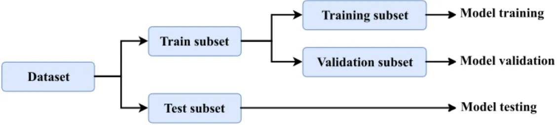
Dataset Train subset Test subset Training subset Validation subset Model training Model validation  Model testing 

Figure 2.2 A typical division of dataset in machine learning. Primarily the dataset is divided into train and test subsets. The train subset is further divided into two disjoint subsets: training and validation subset.

Validation is the technique used in machine learning to monitor the training phase of the model. Validation dataset is used to check whether the trained model is overfitting or not. It evaluates the generalization error during the training process or after training is done. Validation set allows hyperparameter to update accordingly. It helps to minimize the overfitting and the generalization error. Often some portion of the training dataset is reserved to validate the model as shown in Figure 2.2. Common practice in machine learning is to use 20 percent of the train subset to validate the model and 80 percent for solely training the model. [18]

2.2

Deep Learning

Deep learning is the state-of-the-art technology and considered as the major player in the field of AI, machine learning and big data for its outstanding performance. Deep learning is a branch of machine learning. The traditional machine learning techniques strongly influence deep learning [2]. Deep learning is inspired by the concept of artificial neural network and usually consisting of a large number of neural networks (NN). The NN computing systems are inspired by the structure and function of the biological nervous system of an animal brain. Deep learning framework consists of multiple layers of simple modules, the majority of them are used for learning and many of these compute non-linear input-output mapping. The multi-layer model architecture learns the representation of data with multiple levels of abstraction.

Machine learning is good for the structured low dimensionality data and deep learning is used for unstructured, high dimensional data and perceptual problems

[2]. The limitation of linear model to solve high dimensional complex representation has led to the development of more complicated deep models. Machine learning uses single-level representation learning while deep learning uses combination of multiple processing layers to learn the best features needed to represent the data. The higher level of representation learning makes deep learning capable to solve complex task on high dimensional data such as image recognition, text processing and speech recognition [18].

In past, the challenges for the deep learning models were computing resources and large enough datasets to train the model. Easy accessibility of large datasets, availability of powerful computing devices and outperforming graphical processing unit (GPU) plays a significant role behind the popularity of deep learning methods. Modern deep learning models give impressive performance on computer vision, signal processing, speech/audio recognition and natural language processing tasks. [2]

Neural Network

A neural network (NN) is a highly parallel distributed processor that has a natural tendency of storing experimental knowledge and making it available for use. It is related to the function of an animal brain. The principle behind the NN is that knowledge is obtained by the network through a learning process, interconnection strengths (weights) are used to store the knowledge [21]. Neuron, also known as node or unit is the basic building block of artificial NN. The typical combination of neurons is known as a layer. A neuron receives multiple inputs (xi) from sources

connected with it, multiplies each input by the weight of its connection (wi) and

sums them together as shown in Figure 2.3. Often a bias is added to this sum. The sum calculated from the weighted connection is then processed via an activation function. The result is normalized and the output (y) is produced. NN consisting of a large number of hidden layers is known as a deep neural network (DNN).

∑

ᶲ

activation function

y

bias b

Inputs

Figure 2.3 A simple model of artificial neuron.

Activation

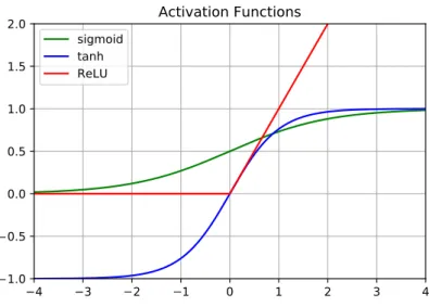
An activation function is used to introduce a non-linearity to the linear activations produced by convolutional (neural) layers and it limits the output of a neuron. Rectified linear unit (ReLU) is used as an activation function in modern CNN archi-tectures. ReLU only passes the positive value and the negative values are mapped to zero as shown in Figure 2.4. ReLU became a popular activation function over sigmoid and hyperbolic tangent (tanh). Meanwhile, the sigmoid function maps the input to values between 0 and 1. Sigmoid function is also known as logistic sigmoid. The tanh function maps input to the value between 1 and -1. ReLU allows fast and effective training of deep neural network on large and complex datasets [17].

4 3 2 1 0 1 2 3 4 1.0 0.5 0.0 0.5 1.0 1.5 2.0

Activation Functions

Figure 2.4 The sigmoid (logistic), hyperbolic tangent (tanh) and rectified linear unit (ReLU) are common activation functions used in Neural Network.

Subsampling

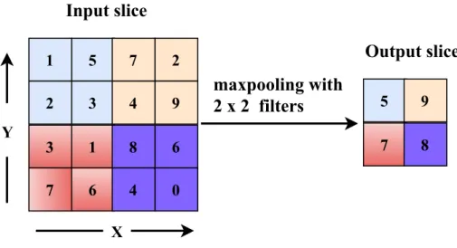
Subsampling shrinks the dimension of input by an integer factor. Subsampling is also known as pooling and is widely used in deep learning. Pooling layers reduce the dimension and resolution of input while preserving the most important informa-tion. Maxpooling, average pooling and L2-norm pooling are examples of sampling technique used in machine learning. Maxpooling is the most commonly used sub-sampling technique where the output is computed as maximum value of input. As presented in Figure 2.5, a small window of dimension 2×2 with stride of 2 is sliding across the two dimensions of data and taking the maximum value from the window at each step. Here 4×4 input data is reduced along both width and height producing output of size 2×2. Pooling reduces the data size and improves the spatial invari-ance to reduce the number of parameters and computation complexity in network. [18] 1 5 2 3 7 2 4 9 3 1 7 6 8 6 4 0 5 9 7 8   X   Y 

Input slice

Output slice

maxpooling with  

2 x 2  filters

Figure 2.5The original image data in X and Y coordinates are down-sampled to half of its original dimension. The2×2maxpooling window with a stride of 2 is applied to the input slice of4×4matrix that reduces to2×2by taking maximum from each window frame. The pooling window size and sliding steps can be changed according to user/application need.

Fully Connected Layer

The fully connected (dense) layer contains weights associated with every input-output pair. This layer combines inner product of weights and the input from every node of the previous layer and translates them into votes. The multidimensional spatial information received from the previous convolutional layers are converted into single feature vector that will help to predict the class probability. This is the

main block on deciding the class label by counting the vote. Usually one or two fully connected layers are connected to learn more sophisticated features from the network in order to make better prediction result. The flattening layer and dense layer are considered as the fully connected layer preceding the output layer. Flattening layer transforms the received multidimensional features into to one dimensional long feature vector. The dense layer reduces the one-dimensional feature vector size and normally makes same size as the number of class category in dataset.

Backpropagation

In NN, input data is passed via the network and the network produces the output. The error is calculated by comparing the output produced by the network and an actual output. The error is used to update the weights of the neurons in order to gradually decrease the error. Backpropagation algorithm is used to solve this issue in training. The goal of the backpropagation algorithm is to make the training error as small as possible. This is done by iteratively passing batches of data through the network and updating the weights. This mechanism is also known as stochastic gradient descent [18].

Backpropagation learning can be implemented in sequential mode or batch mode. In sequential mode, error adjustments are made to the free parameter of the network on one by one basis. Sequential mode is good for classification problems. In batch mode, adjustments are made to the free parameter of the network on an epoch by epoch basis, epochs consist of an entire set of training samples. Batch mode is good for nonlinear regression. Backpropagation algorithm is easy and efficient to implement. However, it is computationally slow for difficult (heavy) tasks. [21, 18]

Feedforward Neural Network

Feedforward neural networks, also known as deep forward networks or multilayer perceptron, are typical deep learning models. The number of layers in feedforward NN ranges from three to thousands. Feedforward neural networks play a vital role in machine learning/deep learning and have been used in many applications. The convolutional neural networks used for object detection are specialized version of the feedforward neural network. In the feedforward network models information from the input flow through the intermediate computation and then result in the final output. The aim of the model is to approximate some function that maps the input to its output. For example, a classifier,y=f∗(x)maps inputx to a category

y. The idea here is to design a mapping function y =f(x;θ) and learn the value of the parameterθ that approximates the best function. In the feedforward neural network, there are typically many different functions composed together which is known as a layer of the network. Functions are connected in a chain forming a deep model. [18]

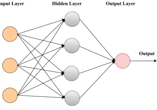
Generally, the feedforward neural network consists of a large number of layers. The very first layer is known as an input layer and the final layer is called the output layer, which are shown in Figure 2.6. Layers between the input and the output are known as hidden layers. The information flow in feedforward is always in one direction (forward) input layer → hidden layer → output layer. In feedforward network the output of the model is never fed back into the network. The feedforward NN which includes feedback connection are known as recurrent neural networks (RNN). Convolutional neural network (CNN) is an example of feedforward neural network.

Input Layer Hidden Layer  Output Layer

Output

Figure 2.6 Fully connected feedforward neural network with an input layer, two hidden layers and an output layer.

The first layer, an input layer is used to prove the input data (features) to the network. The output layer is the final layer in the network that results in the prediction output. The activation function is used in this layer to get the desired output for the problem. Hidden layers are the main block of the model that produces the desired output based on the instruction provided by the learning algorithm. Hidden layer applies various functions to the input. Series of simple functions can

be cascaded to the hidden layers to compute highly complex functions. The number of hidden layers is often termed as the depth of neural network [20].

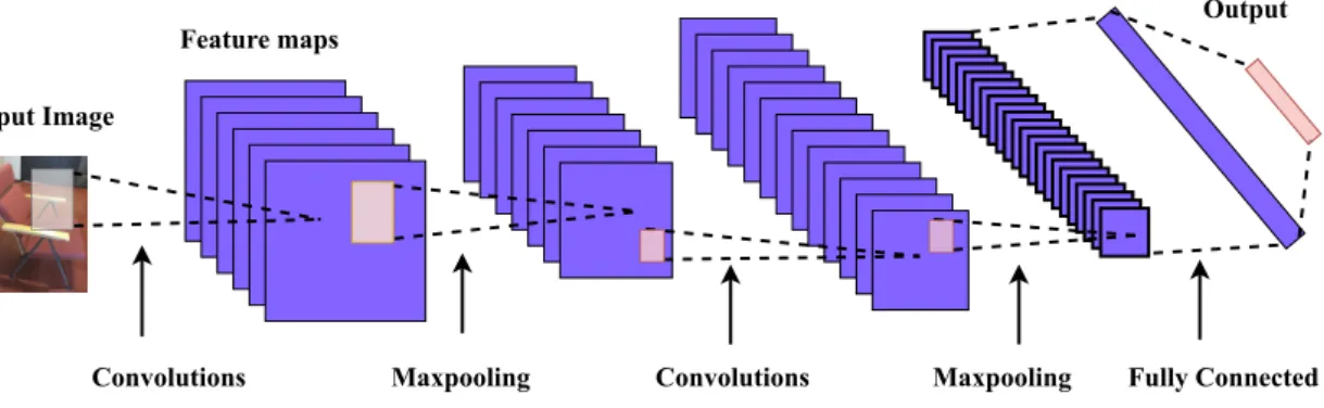
Convolutional Neural Network

Convolutional neural network (CNN) is an artificial neural network consisting of multiple layers also known as neurons. A typical structure of the CNN contains convolution, nonlinearity, subsampling repeatedly connected with fully connected layers. Modern CNN framework consists of a large number of layers (deep lay-ers) containing convolutional and subsampling layers followed by one or more fully connected layers.

Convolution is a mathematical operation on two functions that produces a third function, which is the integral of the product of the two functions with one of them flipped. Convolution is the main building block of the CNN. It is considered as sliding a filter along its width and height. The convolution filter with desired kernel size is applied in input data resulting in the feature maps. Convolution is done at each point of input without overlap. Convolution filters are widely used in image processing, digital signal processing.

Input Image

Feature maps Output

Convolutions Maxpooling Convolutions Maxpooling Fully Connected

Figure 2.7A multi-layer convolutional neural network. An input image is passed through 2 convolution layers followed by maxpooling layers and a fully connected layer and the output layer.

The input image is put through the series of convolution and pooling operations followed by the fully connected layer to produce the output. The convolution filter of fixed size window is applied to each point of image avoiding overlap. The results obtained from these filters are known as feature maps. Maxpooling is applied on each position of these features maps to reduce the dimensionality. The convolution filter is applied again followed by the maxpooling. These processes can be done repetitively many times. Convolutional layers are typically linear, hence, they might

not be able to express possible nonlinearity [48]. The activation function is applied to the output of the convolutional layer to solve the issue of non-linearity. As shown in Figure 2.7, the second last layer, fully connected layer, also known as the dense, layer is used to stack multidimensional output data into a single list. The output layer gets the information from the fully connected layer about the output class associated with the score (frequency) of each class category. [27]

2.3

Assessment Criteria

In machine learning, accuracies measurements are important in order to know how well the machine has learned and how well it performs on unseen data. There are wide ranges of assessment matrices available to measure learning algorithm per-formance. The performance assessment of the object detection model is done by checking how well the model recognizes the object and how precisely it localizes that object. The Intersection over Union (IoU) measure, also known as bounding box overlap, is popular among other assessment approaches [6]. The performance measurement of the object detection model is quantitative and explains to us how many objects are detected correctly and how many objects are predicted wrongly (false alarm).

The overall quality of the object detection model is calculated in terms of IoU,

precision, recall and F1-score. For a large scale multi-class dataset, the mean

av-erage precision (mAP) is used to measure the performance of the method in the

whole dataset [7]. Apart from the accuracy measure, computation complexity of the model is of major concern. The performance of the trained detector on unseen data, training time of the model and processing speed are major factors that need to check while selecting the object detection model from the list of available models. In this thesis, we consider an IoU, precision, recall, F1-score, mAP and frames per second(FPS) as performance assessment criteria for experimented models. IoU, precision, recall, F1-score and mAP are used to measure the correctness of the trained detector while the FPS is used to measure the inference speed of the detector.

2.3.1

Definition of a Detection

The performance assessment of the object detection that uses the bounding box localization method is based on the calculation of the intersection over union (IoU). An IoU is calculated as the ratio of the area of overlap and area of the union. The area of overlap is the total common area or overlap area (i.e. intersection) between

the predicted bounding box (Bp) and the ground truth bounding box (Bgt). The area of the union is the total area covered by both (Bp) and (Bgt).

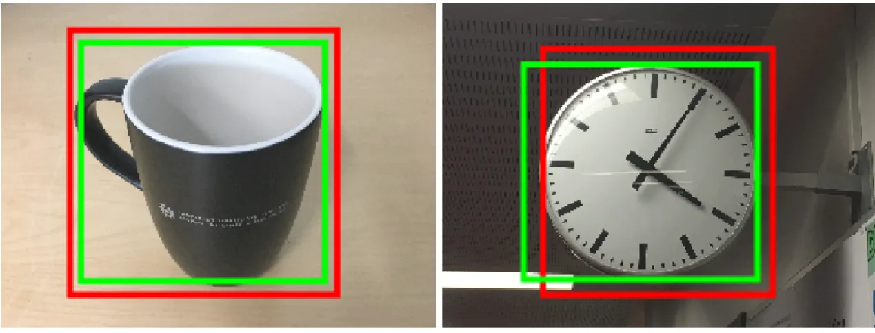
Figure 2.8 Examples of detection of cup and clock with ground truth bounding box drawn in red and predicted bounding box in green. In the left image, the IoU is 0.82 and in the right image, the IoU is 0.73.

Figure 2.8 demonstrates the examples of the predicted bounding box and the ground truth bounding box drawn in the cup and clock classes. The Bgt drawn in red colour is from the annotation file and the Bp in green colour is predicted from the trained detector. Unlike classification problems, object detection accuracy calculation is rather complex. The exact match of the (X, Y) coordinates of the ground truth box and predicted box is extremely rare [39]. For this reason, the object detection performance assessment metric is defined in such a way that the more the Bp overlap with the Bgt the better is the model performance.

An IoU can be calculated when we have the labelled dataset containing ground truth bounding boxes for objects and received prediction for bounding boxes for objects from the trained object detector. The formula to calculate the IoU is given in an equation 2.1. In the numerator, we compute the common area of (Bp) and (Bgt) which is the number of pixels covered by both boxes. In the denominator, we compute total area covered by both boxes.

IoU = area(Bp∩Bgt) area(Bp∪Bgt)

∈[0,1] (2.1)

An IoU is simply the ratio between these two areas. For the correct detec-tion/prediction, the IoU must be greater than the detection threshold value. In object recognition tasks, 0.5 is used as the most commonly acceptable threshold

value above which it is considered as the correct detection [6].

2.3.2

Accuracy Metrics

In machine learning, precision is the fraction of retrieved items over all items that are present. In object detection case, precision is the sum of the correctly detected object divided by the total population of the object that is detected by the detector. Precision takes all the detected object into account.

precision= (relevant objects)∩(retrieved objects)

retrieved objects ∈[0,1] (2.2)

To understand the terms used in performance measurement, it is wise to consider the binary classification problem. The output of the classifier is positive or negative based on whether it is classified correctly or not. The detection of the single object can be considered as classification task. The clear and concise way to understand the idea behind the binary classification accuracy measure is using the confusion matrix, it might be confusing at the beginning as the name suggest.

Table 2.1 visualizes the confusion matrix also known as contingency table. The true class conditions are the ground truth of the data while predicted class conditions are the prediction made by the classifier. The model prediction result will be one of four outcomes, true positives (TP), false positives (FP), true negatives (TN), and

false negatives (FN). Each instance holds two parts, the first part is whether the

prediction is true or false and the second part is the predicted class (positive or negative). If the true class conditions and predicted class conditions are matched, it is considered as TP. If both the real class and prediction class are negative than the result is considered as TN. If the ground truth of the class is positive but the prediction is negative than this instance is called FP. If the prediction is positive but the ground truth is negative than that instance is called FN.

Table 2.1 The 2×2 confusion matrix.

True Class Condition

Positive Negative

Positive True Positive (TP) False Negative (FN)

Predicted Class

Condition Negative False Positive (FP) True Negative (TN)

The diagonal from the upper left to lower right filled with green colour is the correct classification. While another diagonal in red colour is the false classification.

A good classifier must have more instances in the green diagonal than the opposite side, red diagonal. The population of positive class (P) is the sum of all positive instances in data, calculated as,P =T P+F N. The population of negative class (N) is the amount of real negative instances in data, N =T N +F P. Total population is sum of positive and negative classes,T otal(T) =P +N =T P+F N+F P +T N. The amount of false prediction is, (F) = F N+F P.

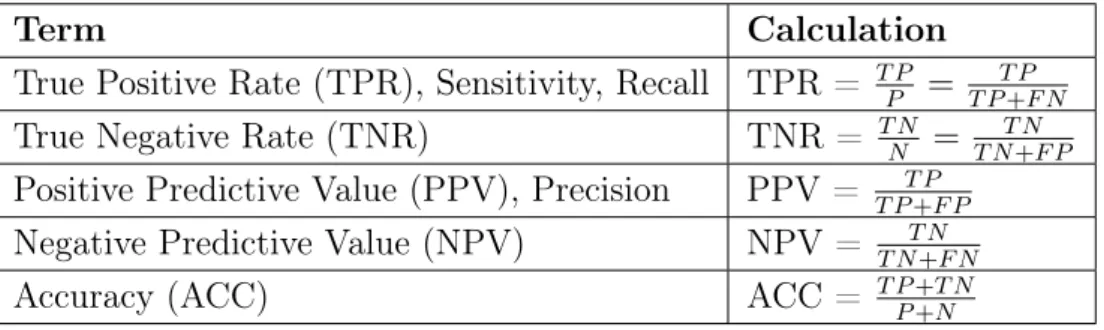
Table 2.2 Calculation of various performance metrics based on the confusion matrix.

Term Calculation

True Positive Rate (TPR), Sensitivity, Recall TPR = T P_P = _{T P}T P_{+F N} True Negative Rate (TNR) TNR = T N_N = _{T N+F P}T N Positive Predictive Value (PPV), Precision PPV = _{T P}T P_{+F P}

Negative Predictive Value (NPV) NPV = _{T N+F N}T N

Accuracy (ACC) ACC = T P_P+N+T N

Many performance measurement matrices can be calculated based on this con-tingency table. Table 2.2 contains the list of most commonly used matrices and their calculations. The calculation of TPR, sensitivity and recall are same. Also, PPV andprecision calculation are same. Anaccuracy (ACC) is the measure of the fraction of correctly predicted instances over total population of instances. The high ACC value is always good for the classification model but is not sufficient to prove that the model is performing well [46]. Sometime the result might mislead. For better performance assessments, we need to consider more accuracy matrices than a single one.

Recall

Recall is the fraction of the relevant items that are successfully retrieved. In the object detection case, recall is the sum of the correctly detected object divided by the sum of actual objects. Recall take only the truly detected object into account. It is also known as the sensitivity of the model.

recall = (relevant objects)∩(retrieved objects)

relevant objects ∈[0,1] (2.3)

F

-score

Precision focuses on accuracy of the model while recall focuses on the robustness of the model. Therefore, calculating the precision and recall alone is not enough

to measure the performance of the model while calculating both gives the better perception of the model performance. F-score combines both precision(PPV) and

recall (sensitivity, TPR) into the single measurement. F-score is the measure of the

accuracy of a classifier also known as F-measure. The formula to F-score based on the confusion matrix is given in the Equation 2.4.

Fβ = (1 +β2)

P P V ×TPR

(β2_{)P P V +TPR} β ∈[0,∞) (2.4)

This can be represented as:

Fβ = (1 +β2)

precision×recall

(β2_{)precision+recall} β ∈[0,∞) (2.5)

where0≤β ≤+∞ and 0≤Fβ ≤1.

Forβ <1, F-score is more precision oriented while for β >1, it is more oriented towards recall. For β = 1, precision and recall are weighted equally, this case is known as F1-score and given by Equation 2.6. The value of β manages significance

of recall over precision. Different value of β can be used based on which metric is important and by what amount. For example, if recall is less important than precision,β <1is used and if recall is more important than precision,β >1is used in the Equation 2.5 [46].

F1 = 2

precision×recall

precision+recall ∈[0,1] (2.6)

F1-score is the weighted average of the precision and recall. Equation 2.6 can be represented as the form of harmonic mean. The value of F1 is bounded between 0

and 1. This indicates that theF1-score is higher only when both precision and recall

values are higher. In multi-class case, it is always worthwhile to calculate the F1 -score as the harmonic mean of average precision and average recall than calculating the mean of individual F1-scores [8].

2.3.3

Mean Average Precision

The mean average precision (mAP) has been widely used to compare the overall accuracies of object detections models on multi-class dataset, since its first intro-duction in Pascal VOC challenge 2007 [7]. The mAP is a single metric that gives the idea about the object detection model performance on the whole dataset. The mAP is not an absolute accuracy metric but it serves as the relative metric. At first, the

average precision (AP) of each class based on different recall values are calculated and then mean of these AP are computed to get mAP of the whole dataset. Dif-ferent techniques are used to calculate the AP. In Pascal VOC, the precision values over 11 values of recall (0.0,0.1 ...,1.0) is used. While in COCO, precision values are computed over 101 different recall values. The calculation steps for mAP based on Pascal VOC is as follow :

1. At first precision and recall are calculated based on the IoU. An IoU greater than the threshold value (usually, 0.5) is considered as true detection.

2. AP is calculated by averaging the maximum precision value at different levels of recall. This is normally taken from the precision-recall curve. The precision values are collected from different recall (11) values ranging from 0.0 , 0.1, ...,1.0. Equations 2.7 - 2.9 show the AP calculation in Pascal VOC [25]. In the COCO dataset, AP is calculated from the precision-recall curve drawn using 101 equally spaced recall values.

AP = 1 11 ×(APr(0.0) +APr(0.1) +...+APr(1.0)) (2.7) AP = 1 11 X r∈(0.0,0.1,...,1.0) APr AP = 1 11 X r∈(0.0,0.1,...,1.0) pinterp(r) (2.8) where, pinterp(r) = max r0_≥r p(r 0 )

The pinterp(r) is the optimal precision for recall values above r.

The simplified equation for AP calculation is: AP = 1

11×(pinterp(0) +pinterp(0.1) +..+pinterp(1.0)) (2.9) 3. Calculate the AP for all object classes present in the dataset.

4. Finally, calculate the mean average precision (mAP) by taking the mean of AP over all the object classes.

The mAP value gives the overall performance of the detector over the dataset, while the AP tells about the performance on a single class. It is obvious that some

classes have higher AP and some classes have moderately low AP. This is due to the number of training samples and (or) quality of samples for each class. The AP result provides the information about whether we need to add/change the training samples in some class or not.

2.3.4

Detection Speed

Computers integrated with high-end GPUs process graphical contents faster than basic computers that only have CPUs or less powered graphics card [32]. Frames per second (FPS) is the frequency of consecutive images, also known as frames, appearing on display. FPS is the widely used metric in broadcasting, film, image and video processing, game, and computer graphics. Computation complexity of the model is one of the main concerns in real-time object detection. There is no clear answer to how much inference speed is considered real-time detection. However, a model is said to be real-time if, its output is faster than or as fast as to the input [32]. The higher the FPS, the better the model performance, but a value less than 1 FPS is considered to be a slow performing model. The inference speed of 1 FPS means every second a single frame is displayed and video of 1 minute contains 60 consecutive frames.

The processing time calculation gives the general information about the com-putation complexity of the algorithm. Deep learning frameworks are complex in nature and computationally heavy. Hence, it is hard to achieve real-time inference on less powerful devices. We considered the FPS as the measure of the computa-tional complexity of the model. As we are running all models in the same work-ing environment, the FPS results give better understandwork-ing of computation cost of experimented models. We compare the computation complexity of experimented object detection detectors during training and evaluation on the test dataset.

3.

OBJECT DETECTION

In this chapter, we discuss the concept of object detection and its applications in modern computer vision. We discuss the convolutional neural networks based object detection architectures and their challenges. Object detection meta-architectures and feature extractors that are used in this thesis project are discussed here.

Background

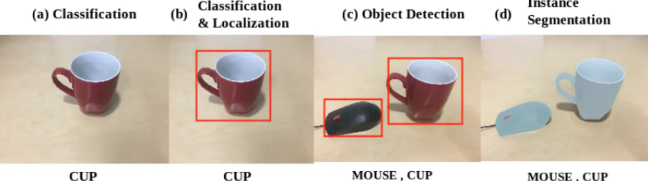
In modern computer vision, object detection is considered together with the object recognition (classification), localization, tracking, and extracting information from the object. These processes are tightly related to the object detection. In clas-sification, the aim is to find out the object class or recognize what the object is. Localization finds the location of the object/s in the image or localizes the object inside the frame. Object tracking in video or live recording is a way to get the move-ment and status of the object. The goal of object detection system is to classify and find the location of all objects that are present in an image. The input for the detector is an image containing the object and the output is a list of the bounding box. Figure 3.1 visualizes the tasks related to object detection. [40]

Figure 3.1 The collection of computer vision tasks related to an object, (a) the classifi-cation (class label) of object in an image, (b) class label of the object and its loclassifi-cation in an image, (c) class and location of each object in an image, and (d) the precise pixels of each object in an image.

Object detection was based on extracting the feature descriptors from the images before the deep learning approaches became prevalent. HOG and scale-invariant feature transforms (SIFT) [33] with support vector machines (SVMs) classification were used for automatic object detection. Deep CNN based models outperform the classical object detection models and are considered as the best performing methods [12]. Faster based convolutional neural network(RCNN) [37], region-based fully convolutional network (RFCN) [5] and single shot detector (SSD) [31] have been used as major meta-architectures in object detection models. These meta-architectures consist of the deep CNN together with the feature extractors. Inception [43], MobileNet [23], NAS [47], ResNet [22] and VGG [42] are popular feature extractors that can be implemented in above mentioned meta-architectures depending on application type and its use in different case.

Object detection is the fast-growing field of research in machine learning and computer vision. The number of problems that can be solved using object detection algorithms is increasing rapidly. Camera-based real-time object detection is on top priority for face detection, object counting, visual/image search, landmark recogni-tion, satellite image analysis, autonomous driving, drone and agriculture productions [9]. Detectron [13], Dlib [28], RetinaNet [29], TensorFlow [44] and You only look once (YOLO) [36] are popular platforms that are used for object detection. Deep convolutional network frameworks are implemented in all modern object detection platforms/libraries.

Challenges

Object detection is known to be a challenging task in computer vision. Large number of training datasets with big number of images from each class category is needed for better learning and generalization. The collection of a large dataset with varieties of objects, scalability of data, the computational complexity of the deep model and the robustness of detector are the main challenges of object detection [35].

Robustness

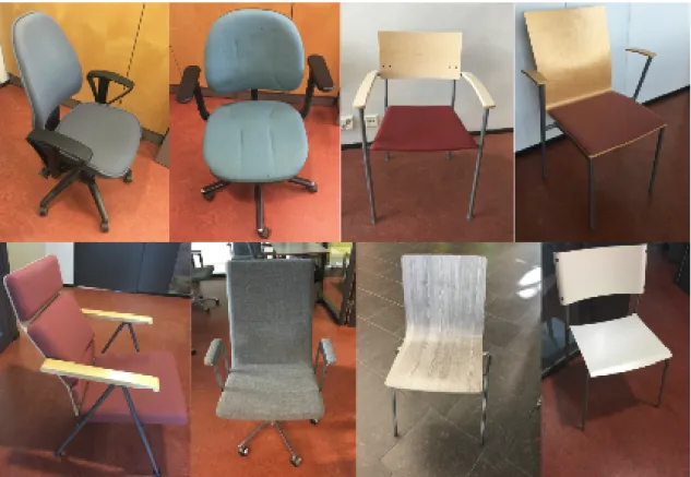
Robustness refers to the challenges of the detector in detecting the object of different appearances. The intra-class and inter-class difference are big challenges for auto-matic object detection [35]. The intra-class difference is the difference between the same class objects, while the inter-class difference is the difference between dissim-ilar class objects. The variation in objects and variation in images are challenging

too. As shown in Figure 3.2, a chair can be of different colour, shape, size and texture. The environments where the images of the chairs are captured are different (background, lighting, and view-angle). The similar appearing object of the dif-ferent class category is another challenge. For example, the inter-class differences of moving chair, sofa chair, armchair and four leg chair are quite small and often considered as common class chairs.

Figure 3.2 Examples of the chair class in our dataset. These are 8 different types of chairs representing single class label (chair). They are captured in different backgrounds, lightings and angles.

Large datasets

The detection model must be complex enough to solve the robustness problem. This necessity motivates to have large dataset and deeper models. The necessity of large-scale datasets to train and test the object detector has been solved by available benchmark datasets. However, these datasets were collected on the specific environment which might not work well in another environment. To make the environment specific object detector, we need to collect a large number of samples from the specific environment for each class category object.

Scalability and Complexity

Another challenge in object detection model is the scalability of high dimensional data. High dimensional data is hard to represent, difficult to train the model and learn the required information. The feature extractors help to solve these issues by extracting only the required features from the data. Most of the modern object detection models use the regional CNN filters to extract the object maps from the input image. CNN architectures are computationally heavy to perform. The hard-ware needed for heavy computation is another challenge in object detection. Easy availability of powerful computing devices, high-end GPUs, parallel computing and cloud-based computing services help to solve this challenge.

3.1

Faster Region-based Convolutional Neural Network

A Region-based convolutional neural network (CNN) has three series RCNN [14], fast RCNN [14] and faster RCNN. Faster RCNN is the latest architecture in the RCNN series and one of the widely used architecture in object detection [37]. Faster RCNN is composed of fully deep convolutional networks that propose regions and the fast RCNN detector, that uses the proposed regions to detect the object. To understand the concept of faster RCNN it is wise to go through the principle behind the RCNN. RCNN is a three-stage process. At first, a selective search algorithm is used to scan the objects in input image known as region proposal. The convolutional neural network is run on top of each of these region proposals. The third stage is to feed CNN output into support vector machine (SVM) to classify the object region and a linear regression is used to tightened the bounding box of the object. [37]

In faster RCNN, slow selective search algorithm implemented in RCNN is replaced with a fast-neural network. The detection in faster RCNN is a two-stage process. At first, a convolutional filter is run through the entire image resulting in the feature maps. The region proposal network (RPN) is applied on those featured maps and output the set of object proposal boxes with scores. Image feature maps achieved from the convolutional filter are used to predict the object proposal with scores. Object proposal network is proposing boxes based on the intersection over union (IoU) between the purposed object and the ground-truth object. In the next stage, object proposal extracts the area of the object from the feature maps. This is done by region of interest (RoI) pooling layer. The extracted features are applied to all layers of feature extractors to get the prediction probability of the class and the bounding box for each region proposal. The final stage is to classify the object and its location (bounding box) found in the image. As shown in Figure 3.3, entire

Figure 3.3 Single unified network for object detection implemented in faster region-based convolutional network model [38].

operation occurs on the unified single network, that enables the system to apply convolutional filters together with the detection network. It is proven that faster RCNN meta-architecture with a good feature extractor has excellent performance on complicated object recognition and classification challenges [9].

3.2

Region-based Fully Convolutional Network

The region-based fully convolutional network (RFCN) uses two-stage object detec-tion strategy consisting of regional proposal and region classificadetec-tion. RFCN is identical to faster RCNN but instead of cropping features from the predicted re-gional proposals, features are taken from the last layer of features preceding the prediction. This technique helps to minimize the quantity of memory applied in region computation. It was mentioned that RFCN together with the ResNet101 feature extractor has competitive performance compared to faster RCNN [9, 5].

The architecture of RFCN is shown in Figure 3.4. At first, the convolutional filter is applied over the input image. The fully convolutional layer is added to generate a score of positive-sensitive score maps (feature maps). The fully convo-lutional regional proposal network (RPN) generates the regions of interest (RoI) from the previous layer output (feature maps). Each generated RoI is divided into subregions (bins) as scored maps. The score bank of each bin is compared with the corresponding position of the object. The process is repeated for all the bins and for all the classes presented in the image. When these bins have an object matched with

Figure 3.4 Regional based fully convolutional network meta-architecture. Input image is gone through the convolution and RPN proposes the possible regions of objects. RoI pooling is applied to RPN outputs and finally classifier classify the object [5].

enough of sub-region of the object, the average score is calculated per class. At the final stage, softmax pooling is used to classify the object class based on the previous vote from the RoI layer. RFCN is fully convolutional and shares the computation throughout the networks which make this model faster than the faster RCNN model [5].

3.3

Single Shot MultiBox Detector

A single shot multi-box detector (SSD) meta-architecture solves the object detection problem by using a single pass of a feedforward convolutional network. Unlike other models, this does not generate region proposals nor do resampling of image segments thus saving computational time [9, 31]. This network handles objects of different sizes by using features maps from different convolutional layers as input to the classifier. This network produces a large number of bounding boxes with the scores of object class in those boxes. Non-maximum suppression is used to eliminate boxes below a certain threshold so that only the boxes with higher confidence values proceed for classification. SSD meta-architecture allows end-to-end training and improving the speed of the detector. This meta-architecture does everything in one shot, thus, it is faster than other meta-architectures but it lags the detection accuracy.

body class predictor box predictor down sample class predictor box predictor

input  scale 0  scale 1

Figure 3.5 SSD layer is series of small convolutional layer that is added on top of base layer [15].

The SSD layer architecture is built on top of a feedforward CNN that results a fixed-size collection of bounding boxes and object class instances present in those boxes. The input image is passed through a series of convolutional layers and down-sampled via the SSD layer shown in Figure 3.5. This SSD layer is linked to the output of the last convolutional layer of the base model. Multiple sets of feature maps at different scales are achieved from the convolutional layers with the predic-tion of object classes (from class predictor) and set of bounding boxes (from box predictor). The predicted boxes are compared with the ground truth of the object and the best one with higher IoU is selected together with the higher probability score from class predictor.

3.4

Feature Extractors

The feature extractor is the major building block of the object detection model that is used to extract the features of objects from the data. The object detection model structure is composed of detection meta-architecture, feature extractor and classifier as shown in Figure 3.6. The input image is passed through the feature extractor that extracts features from the image. The extracted features are then forwarded to the classifier that classifies the class and the location of the object in the input image.

Feature   Extractor Classifier Input Image Class Localization Meta­architecture

Figure 3.6 Object detection model architecture is composed of the feature extractor and classifier in meta-data architecture [9].

The feature extractor is a deep architecture that aims to increase the accu-racy while reducing the computational complexity. AlexNet, Inception, Mo-bileNet, NAS, ResNet and VGG are some popular feature extractors that can be implemented in object detection meta-structures. We used the Inception, MobileNet, ResNet and NAS feature extractors implemented in above-mentioned meta-architecture.

Inception

The inception module works as multiple convolution filters that are applied to the same input together with pooling and concatenation to get the result. Inception architecture allows the model to gain advantage from the multi-level feature extrac-tion.

1 x 1 convolutions 3 x 3 convolutions 5 x 5 convolutions 3 x 3 max pooling

Filter concatenation

Previous layer

Figure 3.7 Inception module, naive version [43].

Inception module uses a combination of compositions of different convolution filters. At first, the 1×1convolution is followed by the various size of convolution

filters (3×3convolutions and 5×5 convolutions) and maxpooling operation. The output from these filters and pooling are concatenated to get the final result as shown in Figure 3.7. Inception network is the combination of numbers of this inception module. It is believed that getting multiple features from multiple filters improves the performance of the network.

Mobile Network

Mobile network (MobileNet) is a lightweight deep neural network that is efficient for mobile and embedded devices. The principle behind this architecture is the division of the standard convolutional filter into two convolution filters, depthwise convolution and pointwise convolution (1× 1 convolution). The computation com-plexity of the standard convolutional filter is higher than the combined computation complexity of depthwise and pointwise convolutions.

. . . . . . . . .    N     N     M   M M D D 1 1 (a) Standard Convolution Filters (b) Depthwise Convolution Filters (c) Pointwise Convolution Filters 1 D D

Figure 3.8 MobileNet feature extractor is based on the separation of the standard convo-lutional filters into depthwise convolution and pointwise convolution [23].

The computation cost of the convolution depends on the input network (M), size of the output network (N), feature map size (DF ×DF) and the kernel size

(DK×DK). The computation complexity of the standard convolutional filter shown

in Figure 3.8 (a) is higher than the total computation cost of the depthwise (b) and the pointwise (c) convolution filters. This division is optimized for the computation

speed. The reduction in accuracy is rather small in comparison to the to the standard one. These are the parameters for balancing between speed and accuracy. [37]

Residual Network

Residual Network (ResNet) is based on the residual learning principle. The idea is to learn a residual instead of the features. The deep residual network consists of 152 residual blocks [22]. ResNet is the record breaker a single architecture for classification, detection, and localization tasks. It surpasses a human on ILSVRC 2015, ImageNet and COCO 2015 competitions with an incredible accuracy and is known as the best CNN architecture [26]. The increase in depth of the deep NN increases the accuracies until some point and after that, it starts decreasing. Residual learning tries to solve this issue of accuracy degradation in NN [22].

weight layer weight layer

+

Figure 3.9 F(X) is the residual function of non-linear CNN layers. In the plain block (a), it is difficult to get identity mapping by pushing the residual function to zero. It is easier to get identity mapping in the residual block (b) than in the plain block (a) [26].

The idea behind the ResNet architecture is to use a residual function instead of direct mapping of input-output. The residual function is F(x) = H(x)−x where F(x) is the stacked non-linear layers, H(x) is mapping function and x is identity function. This residual function can be re-framed to H(x) = F(x) +x. It is easier to get the residuals to zero than to fit an identity (input = output) mapping using stacks of non-linear CNN layers as the function.

4.

IMPLEMENTATION

This chapter presents information about data collection, annotation and preprocess-ing needed to train the object detection models. The environmental setup needed to train and test the object detection models from TensorFlow object detection model zoo is discussed here. Data collection, annotation, preprocessing and the formation of the train-test dataset are of major concern in object detection.

4.1

Dataset

Data is the core necessity to train, test and validate any kind of machine learning task. Especially in supervised machine learning, we need labelled data that will determine what our algorithm will learn and predict as a result. The training data is the major factor that influences the model behaviour and performance on unseen data. The data processing stage includes the collection of the datasets, the annota-tion and formaannota-tion of the train and test subsets. This secannota-tion describes the methods used for data collection, annotation and preprocessing to achieve our experimental goal.

4.1.1

Data Collection

The data used in this project were collected during this project. The first stage of data collection was recording videos in the university premises including corridors, labs, meeting rooms and offices. From the series of recorded videos, interesting frames were extracted. The deep learning implementation needs way more training data than the basic machine learning algorithms. During the collection of our object detection dataset, we faced some challenges. One of the major challenges was the collection of common objects suitable for the dataset. The quality and clarity of images and objects was an issue itself. This challenge was solved by using the better quality video recorder. The collection of varied sets of images of the same object was another challenging task during data collection. Manually annotating all objects and their instances with the corresponding class labels was another challenge.

We extracted 1100 frames from the series of recorded videos inside TUT premises. In each captured frame there were one or many objects of single/multi-class instance. In addition to self-collected data, 40 images of remote controls and 25 images of exit signs were downloaded from Google image search.

Figure 4.1 Sample images with different objects from our dataset. These were captured in various indoor premises at TUT.

Table 4.1 List of the objects in our dataset based on the class category.

Category Object Instance

Natural Human Plant Flower

Furniture Box Boxes Chair Door Drawer Sofa Table Electronic Clock Printer Remote Screen Socket Switch

Other Bike Board Cup Exit Fire ext. Picture Trash bin

Our dataset contains 23 classes of interesting objects found at TUT indoor premises such as human, small plants, furnitures, safety symbols (fire extinguisher and exit) and electronics goods. Figure 4.1 presents some representative images from our dataset. Table 4.1 lists class label of the objects in our dataset. These images were taken from indoor TUT premises on diverse backgrounds, lighting conditions, sizes and viewpoints.

4.1.2

Data Annotation

Data annotation is the process of labelling the data for supervised machine learning method. In case of object detection, an annotation is a process of localizing the object inside the given frame and labelling it. Bounding box approach and the pixel-wise object segmentation are two methods used to annotate the object on the image frame. We used the bounding box annotation approach where the bounding box is drawn locating the object, a rectangular box is drawn around the object boundary making object inside the drawn box. Dlib image annotation tools Imglab 1_{was used to annotate the images. The information of the images and corresponding} boxes were stored in a file and saved in extensible markup language (XML) .xml

format. The XML file format created using the Imglab tool contains the image file with the information of rectangular box around the object and the corresponding class label of the object/s.

Figure 4.2 Screen capture of Imglab graphical user interface(GUI) during multi-class object annotation.

The screen capture of Imglab graphical user interface (GUI) is shown in Figure

1