Learning Multimodal Structures in Computer Vision

(1)

University of Tennessee, Knoxville

Trace: Tennessee Research and Creative

Exchange

Doctoral Dissertations Graduate School

8-2017

Learning Multimodal Structures in Computer

Vision

Ali Taalimi

University of Tennessee, Knoxville, [email protected]

This Dissertation is brought to you for free and open access by the Graduate School at Trace: Tennessee Research and Creative Exchange. It has been accepted for inclusion in Doctoral Dissertations by an authorized administrator of Trace: Tennessee Research and Creative Exchange. For more information, please [email protected].

Recommended Citation

Taalimi, Ali, "Learning Multimodal Structures in Computer Vision. " PhD diss., University of Tennessee, 2017. https://trace.tennessee.edu/utk_graddiss/4714

(2)

To the Graduate Council:

I am submitting herewith a dissertation written by Ali Taalimi entitled "Learning Multimodal Structures in Computer Vision." I have examined the final electronic copy of this dissertation for form and content and recommend that it be accepted in partial fulfillment of the requirements for the degree of Doctor of Philosophy, with a major in Electrical Engineering.

Hairong Qi, Major Professor We have read this dissertation and recommend its acceptance:

Mark Dean, Seddik Djouadi, Jens Gregor, James Ostrowski

Accepted for the Council: Dixie L. Thompson Vice Provost and Dean of the Graduate School (Original signatures are on file with official student records.)

(3)

Learning Multimodal Structures in

Computer Vision

A Dissertation Presented for the

Doctor of Philosophy

Degree

The University of Tennessee, Knoxville

Ali Taalimi

August 2017

(4)

c

by Ali Taalimi, 2017

(5)

(6)

Acknowledgments

This dissertation would not have been possible without the guidance and support of several individuals who have extended their valuable assistance in the completion of my Ph.D. studies. First, I would like to express my sincere appreciation and gratitude to my advisor, Dr. Hairong Qi, for giving me the opportunity to be part of her research group. I am especially thankful for her continuous support of my study and research, and also for her kindness, patience, motivation, and enthusiasm. Her calm and friendly attitude combined with her immense knowledge of this field made my learning process and research experience much more enjoyable. Second, I would like to thank my dissertation committee members, Dr. Dean, Dr. Djouadi, Dr. Gregor and Dr. Ostrowski for all the support, guidance, and understanding. I really appreciate their insightful comments about my dissertation and great discussions that we had about my research problem.

My friends and labmates were also an integral part of my research experience. I want to thank them all for their comments and suggestions and wish them all the best in their research and career. Last, but certainly not the least, I would like to dedicate this dissertation to my parents Shirin and Ali Mohammad, and my wife May. I could not have accomplished this without their love and constant support through tough times.

(7)

Abstract

A phenomenon or event can be received from various kinds of detectors or under different conditions. Each such acquisition framework is a modality of the phenomenon. Due to the relation between the modalities of multimodal phenomena, a single modality cannot fully describe the event of interest. Since several modalities report on the same event introduces new challenges comparing to the case of exploiting each modality separately.

We are interested in designing new algorithmic tools to apply sensor fusion techniques in the particular signal representation of sparse coding which is a favorite methodology in signal processing, machine learning and statistics to represent data. This coding scheme is based on a machine learning technique and has been demonstrated to be capable of representing many modalities like natural images. We will consider situations where we are not only interested in support of the model to be sparse, but also to reflect a-priorily known knowledge about the application in hand.

Our goal is to extract a discriminative representation of the multimodal data that leads to easily finding its essential characteristics in the subsequent analysis step, e.g., regression and classification. To be more precise, sparse coding is about representing signals as linear combinations of a small number of bases from a dictionary. The idea is to learn a dictionary that encodes intrinsic properties of the multimodal data in a decomposition coefficient vector that is favorable towards the maximal discriminatory power.

We carefully design a multimodal representation framework to learn discriminative feature representations by fully exploiting, the modality-shared which is the information shared by various modalities, and modality-specific which is the information content of

(8)

each modality individually. Plus, it automatically learns the weights for various feature components in a data-driven scheme. In other words, the physical interpretation of our learning framework is to fully exploit the correlated characteristics of the available modalities, while at the same time leverage the modality-specific character of each modality and change their corresponding weights for different parts of the feature in recognition.

(9)

List of Tables

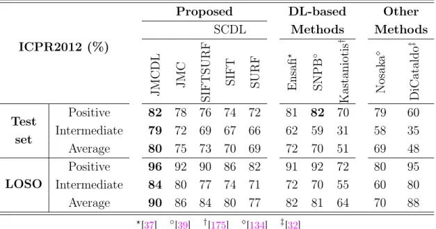
2.1 The MCA accuracy on ICPR2012 dataset by using two evaluation strategies “Test set” and “Leave-One-Specimen-Out (LOSO)” for Cell Level classification (Task 1). . . 40 2.2 The MCA accuracy on ICPR2012 dataset by using two evaluation strategies

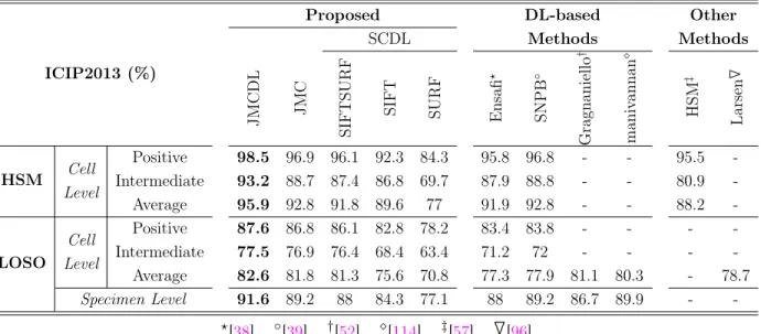
“Test set” and “Leave-One-Specimen-Out (LOSO)” for Specimen Level classi-fication (Task 2). . . 41 2.3 The MCA accuracy on ICIP2013 dataset by using two evaluation strategies

“HSM” [57] and “Leave-One-Specimen-Out (LOSO)”. . . 42 2.4 The Cell Level confusion matrices by using Leave-One-Specimen-Out method. 43 2.5 The comparison of proposed SCP with SPM strategy by using different pooling

functions and using LOSO evaluation method On Cell Level (Task 1). . . 44 3.1 The average overlap score of 5 trackers on 7 different videos. The best is

shown by red and blue is the second best. . . 73 3.2 Precision (Center Location Error) in OTB-100 (sequence average). The

trackers are ordered by the average overlap scores, and the top 5 methods in each attribute are denoted by different colors: red, green, blue, cyan,

(13)

3.3 Success rate (overlap) in OTB-100 (sequence average). Each entry contains the average overlap in percentage at the overlap threshold of 0.5. The trackers are ordered by the average overlap scores, and the top 5 methods in each attribute are denoted by different colors: red, green, blue, cyan, and

magenta. . . 81

3.4 Comparing the best trackers of OTB-100, and Deep Learning trackers with MM-THM using Precision rate (Center Location Error) in OTB-100 (sequence average). Each entry contains the average overlap in percentage at the overlap threshold of 0.5. The trackers are ordered by the average overlap scores, and the top 5 methods in each attribute are denoted by different colors: red, green,blue,cyan, and magenta. . . 82

3.5 The best trackers of OTB-100, and Deep Learning trackers are compared with MM-THM using Success rate (overlap) in OTB-100 (sequence average). Each entry contains the average overlap in percentage at the overlap threshold of 0.5. The trackers are ordered by the average overlap scores, and the top 5 methods in each attribute are denoted by different colors: red, green, blue, cyan, and magenta. . . 83

4.1 The gender classification accuracy (%) with p= 250. . . 120

4.2 Gender classification rates obtained with p= 25 atoms. . . 120

4.3 Face recognition accuracy with the whole face modality . . . 121

4.4 Recognition performance of each single modality in AR database. Modalities include left periocular, right periocular, nose, mouth, and face. . . 122

4.5 Modalities include 1. left periocular, 2. right periocular, 3. nose, 4. mouth, and 5. face. . . 123

4.6 Multimodal face recognition results for the AR dataset . . . 123

4.7 Multiview face recognition results for the UMIST datasets . . . 125

(14)

4.9 Evaluation of MWDL, JTLDL and HTLDL for the recognition rate on “large-baseline” evaluation of BMW . . . 127 4.10 Multiview action recognition on the IXMAS (%) . . . 129

(15)

List of Figures

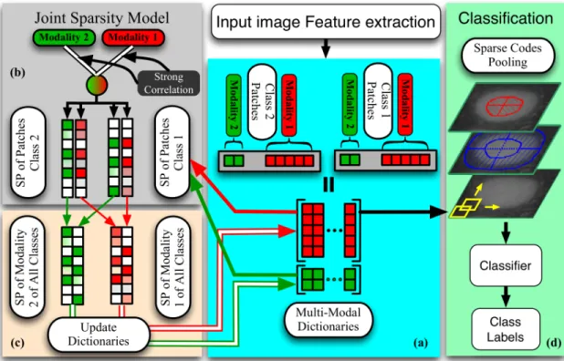
2.1 The illustration for the joint sparse modeling for classification task of two classes with two modalities: (a) The patches from two classes have M = 2

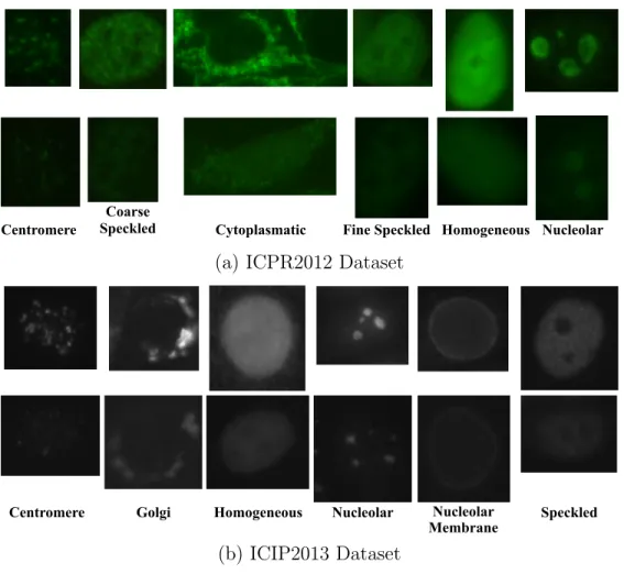
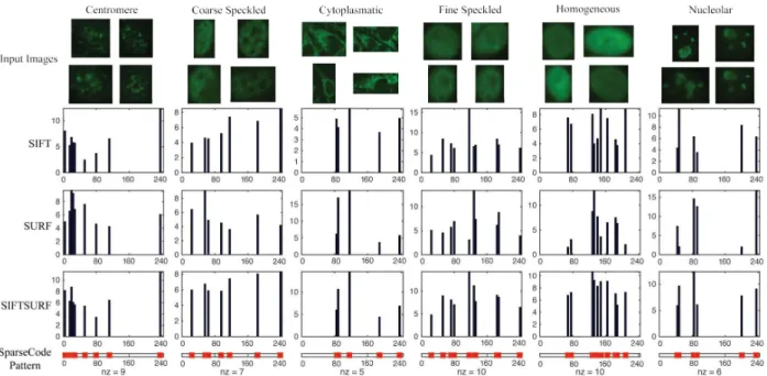
modalities that are shown as red and green. There is a color coded dictionary corresponding to each modality. The multimodal sparse representation of each patch is obtained by multimodal dictionaries _{Dm}Mm=1 and joint sparsity regularization. The entries of sparse codes have different colors and represent different learned values; the white entries indicate the zero rows and columns. (b) The joint sparsity regularizer that is used to impose high correlation between the sparse representation of a sample in two modalities of {red,green_}. (c) Modality-based sparse codes of all classesXm = [x1m,x2m]is used to updateDm. (d) The sparse code polling method is used to aggregate local sparse codes and train the SVM classifier in training stage. . . 30 2.2 SPM method. . . 35 2.3 Proposed SCP method. . . 35 2.4 The Cell Level images of six classes for the ICPR2012 dataset in (a) and the

ICIP2013 dataset in (b): First rows are the positive and second rows are the

(16)

2.5 Representation coefficients generated by proposed regularization for SIFT, SURF and SIFTSURF features. There are six columns corresponding to the six classes. The x-axis is the dictionary columns and the x-axis is the sparse code values corresponding to each dictionary column. nz is the number of

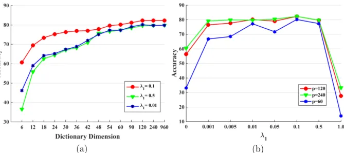
non-zero elements in the sparse code vector. . . 44 2.6 The accuracy of ICPR2012 positive test set versus different dictionary atoms

in (a) and λ1 values in (b). . . 45 3.1 Illustration of independent vs overlapped coupling. Consider the case with

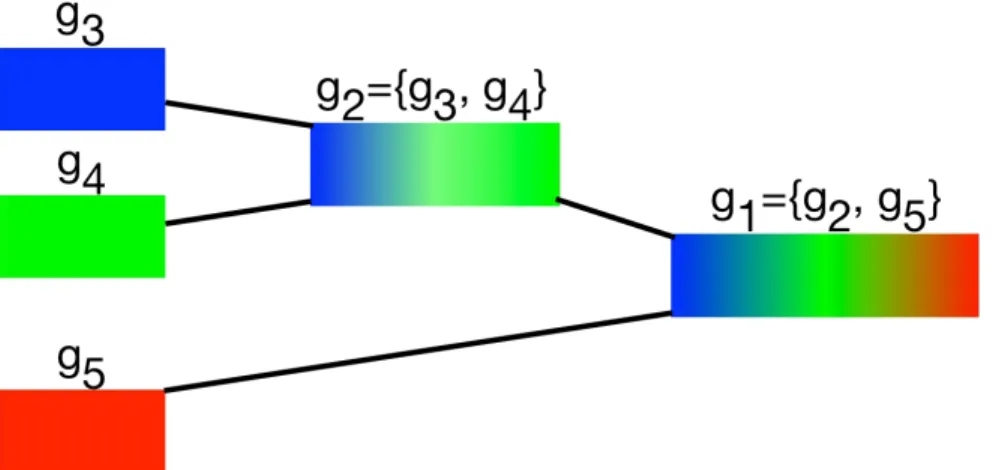
M = 3 modalities of red, green and blue. (a) shows a multimodal signal X = _{xred,xgreen,xblue} that has a mixture information of mostly red and a smaller amount of green. (b) a multimodal atom _{d_} = dred,dgreen,dblue. The goal is to decompose the multimodal input X using _{d_} to multimodal coefficients A = [αred,αgreen,αblue]. (c) the result of independent coupling using `12. All three values of decompositions are equal. (d) the result of overlapping coupling. The αred αgreen and αblue= 0. . . 51 3.2 Illustration of a hierarchical structure between various modalities of input

data. The tree is _G = {g5, g4, g3,{g3, g4},{g2, g5}}. It has three leaves of {g3, g4, g5}, and g2 enforces coupling between g3, g4, and the root of the tree g1 enforces grouping between g2 and g5. Internal nodes near the leaves of the tree correspond to modalities that we expect highly related while the internal nodes near the root represent weakly-correlated sparse codes in its subtree. Any path from leaves to the root, is a possible solution. . . 53

(17)

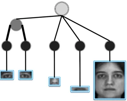
3.3 Illustration of joint sparsity vs tree-structured grouping. Consider the case with M = 3 modalities of red, green and blue. Top: `12 all modalities are in one group. Down: The tree-structure regularization enforces hierarchical fusion between various modalities of input data in the space of sparse codes. The tree is _G = _{g5, g4, g3,{g3, g4},{g2, g5}}. It has three leaves {g3, g4, g5}, and g2 enforces grouping between g3, g4, and the root of the tree g1 enforces grouping between g2 and g5, and is a hierarchical grouping between red and the group of blue and green. The key here is that partially correlated coupling is not allowed in the tree structure. The groups of variables either are independent or one is subset of the other. . . 54 3.4 We employ the blue rectangular masks and cropping out the corresponding

areas. These, along with the whole face, were taken for fusion. Simple intensity values were used as features for all of them. Tree-structure _G corresponding to the four weak modalities of left periocular, right periocular, nose, and mouth, and a strong modality face. The tree represents a set of groups_G between left and right periocular and all modalities at the root. . . 55 3.5 Illustration of intersection closed coupling. The tree-structure _G

correspond-ing to the four weak modalities of left eye, right eye, nose, and mouth, and a strong modality face, _G ={g1, g2, g3, g4, g5, g6, g7}. If variable left eye is non-zero, i.e. a(g3) ₆_{= 0},then automatically, _g

2 is non-zero, and also the root g1 is selected. This path fromg3 →g2 →g1 is a valid solution with three activated groups out of total 7 groups. This solution gets high punishment from reconstruction part of the optimization problem. Intuitively, each interior node that is activated, hereg2, favors to see all of its members, (g3 and g4) to be non-zero, to get less reconstruction punishment. . . 58

(18)

3.6 Illustration of the proposed MM-THM framework. Tracking can be seen as a binary classification of target and background. Consider each patch has M

different modalities. Originally, the physical attributes are not discriminative enough to distinguish the target from the background. Our method learns a set of dictionaries to find the representation of data in latent space of sparse codes, to make the target more distinctive in each modality, and, from multimodal stand-point. . . 61 3.7 The hand-coded tree-structure norm-based regularization in space of sparse

codes for MM-THM. This tree has M = 7 leaves (features) and 5 groups.

From left to right: fhog, HSV and CIE Lab channels. . . 71 3.8 Tracking results of selected11trackers in representative frames. Frame indices

are shown in the top left of each figure. The showing examples are from sequences carDark, Jogging, Singer1, Bolt, Walking2, Basketball, respectively. 73 3.9 (a) precision and (b) success plots for the 50 videos with all available trackers

in the benchmark OTB-50. The proposed MM-THM achieves overall the best performance in both metrics and outperforms the second best tracker SMS and SCM more than 10% and 15%, respectively. . . 74

3.10 (a) precision and (b) success plots for the 50 videos with all available trackers in the benchmark OTB-50 and recent high-performance trackers in [92]: CN [30], MUSTer [61], KCF [59] and MEEM [204]. The proposed MM-THM outperforms MEEM by8.2%and has similar performance with MUSTer

in success plot and also achieves third best overall performance in precision plot with precision 3.26% less than MUSTer. . . 75

3.11 (a) precision and (b) success plots for the 100 videos with all available trackers in the benchmark OTB-100. The proposed MM-THM achieves overall the best performance in both metrics and outperforms the second best tracker SMS and STRUCK more than 5% and 13%, respectively. . . 76

(19)

3.12 Comparison with state-of-the-art deep learning trackers. (a) precision and (b) success plots trackers in the benchmark OTB-100. . . 77 3.13 Comparing MM-THM in precision plot with trackers in OTB-100 in all

attributes. The score for each tracker is shown in the legend. The top 10 trackers are presented for the sake of clarity, and the rest are shown as gray dashed curves. . . 78 3.14 Comparing MM-THM in success plot with OTB-100 trackers in all attributes.

The score for each tracker is shown in the legend. The top 10 trackers are presented for the sake of clarity, and the rest are shown as gray dashed curves. 79 4.1 Samples of male and female with extracted modalities in AR dataset. . . 121 4.2 We employ the blue rectangular masks and cropping out the corresponding

areas. These, along with the whole face, were taken for fusion. Simple intensity values were used as features for all of them. Tree-structure _G corresponding to the four weak modalities of left periocular, right periocular, nose, and mouth, and a strong modality face. . . 122 4.3 Illustration of 3 view-range (modalities) in UMIST. Different poses of a subject

from UMIST database. Each row is a view-range or modality for the subject. 126 4.4 (a) Apparatus which instruments five camera sensors [129]. (b) Five “large

baseline” images captured at different vantage points. . . 126 4.5 Check watch action sample from the IXMAS dataset [183]. Each action is

(20)

Chapter 1 Introduction

1.1 Motivation and Background

A significant amount of studies in signal and image processing has been done to represent signals in a proper fashion for the specific task. Restoration in general and in particular denoising and reconstruction are emerging estimation problems in these fields; that may become difficult to solve without an arbitrary a priori model of the data source. In machine learning and computational statistics, various research tries to answer the question of how to learn a set of parameters from data while a predefined criterion is maximized, in both a supervised or unsupervised scheme. For instance, to find the connection between input data and output response, or when one may need to summarize (compress) the data.

A simple a priori model is to assume the solution to be sparse. This bias towards sparsity can emerge in two scenarios: First, we know that the problem at hand has a sparse solution, or in the absence of sparsity prior information, our interest lies in seeking a simple reasoning for the task that is easy to interpret and has a low processing complexity. This is known as sparsity and can be assumed as selecting a small number of parameters to solve the problems. In early studies, a pre-defined dictionary is used which was made out of a set of orthonormal basis. Then, the signal can be represented using a linear combination of the dictionary elements also known as atoms.

(21)

The dictionary should be designed so that it can successfully reconstruct the data while at the same time, has a poor performance in modeling the noise. In that case, the sparse decomposition coefficients and the dictionary together may have a good representation out of the pure signal. That is, to obtain a proper representation of the signals, the design of the dictionary has a significant role and is an active topic of research.

Let us emphasize on the difference between the terminology models in this dissertation

with generative models. We use this terminology to define classes of regularized signals that

we design to have interesting characteristics, but it may also have irrelevant representations. However, in generative settings, models are the probability distribution of input data.

The dictionary in statistics and machine learning may be simplified as a set of fixed variables or predictors and then seeking for the solution as a linear combination of variables in the dictionary. However, the method should be designed so that it can successfully generalize the unseen and new data; that is to make sure that the model does not suffer from the overfitting problem. It can occur due to a large number of basis or a small number of training samples. The prior information about the data or the form of the solution leads to the concept of regularization that shows promising results to deal with the overfitting problem. For instance, the Tikhonov regularization that favors towards a smooth solution is a well-known prior among various fields. In this dissertation, the sparse solutions are preferred, which leads to `1-norm regularization. Particularly, beside the sparsity, we are

interested in encoding different prior information over the data or the characteristics of the solution in the pattern of the non-zero coefficients. Sparse models have been successfully applied in the recent two decades in many scientific disciplines: simple model selection out of a pool of possible choices is done using the sparsity principle in statistics and machine learning. Sparsity models try to explain the observed data by selecting a few predictors (atoms of the dictionary). In signal processing, sparsity is used to approximate signals as a linear mixture of a small number of dictionary elements, imposing a union-of-subspaces model on the data. Sparse coding representation has been the topic of a large amount of work in image processing and computer vision.

(22)

Classification is a well-known problem in computer vision and machine learning com-munities. The classification accuracy is mostly investigated from one individual source of information. However, any source of information is limited to its neighborhood, and its efficiency is bounded, and they are prone to be corrupted and become unreliable. So, making decision relying on a single source can jeopardize the decision making process [179,31]. One solution is to use multiple sources of information when it is possible. The information fusion is split into two broad categories: feature fusion [151] and classifier fusion [153, 164]. In feature fusion, we have features at the input and output of the fusion process. The goal is to make or improve a new feature type from input features. The fusion system has various extracted features from each source at the input level. Classification is done based on the new feature set obtained at the output of the fusion process. That is why feature fusion is called feature in-feature out (FEI-FEO), as well. The simplest way of feature fusion is by concatenation of different features into a vector. In [190] different features from wearable sensors are concatenated to a longer vector to do action classification. In classifier fusion, a classifier that is trained based on each feature type makes its decision. The fusion system combines input decisions to obtain better or new decisions. For example, in [150, 81, 83] classifier fusion is applied in majority voting fashion [219, 82] in biometric recognition using classifiers built based on iris, finger and face data. Beside majority voting, different mixing policies like Bayesian inference are used to do the fusion [93].

The majority of studies in information fusion are based on classifier fusion. However, it cannot fully exploit the cross-correlation between multiple sources of information because each classifier is local and is independent of others. On the other hand, feature fusion showed to get superior performance than classifier fusion in the presence of highly related feature modalities [88]. However, the design of the feature fusion system is more challenging especially when the size of features are not the same. The easiest way to fuse different features is to concatenate them in one large vector. This method has two major drawbacks: 1. The new feature vector is large that may lead to the curse of dimensionality especially

(23)

when training data set is small. 2. it neglects the useful cross-correlation information and even may contain noise and outlier which is reported problematic in noisy environments [151]. Our focus in this dissertation is to creating a joint multimodal representation by embedding the representation of every single-modal into a common (latent) representation space. There are two main groups of such approaches:

1. The initially disjoint modalities are exploited to create a joint representation. The goal of this step is to make a proper representation in the latent space. To be concise, this step does not necessarily provide a bidirectional mapping. In other words, we do not necessarily seek to regenerate original physical space from joint multimodal latent space. These approaches are typically used in retrieval and classification tasks.

2. Bi-directional mapping is mainly discussed in cross-modal approaches, which may or may not include learning a joint representation space. The main focus is to generate one modality from the latent representation of another modality and back, as well as represent them in a joint representation space. These methods are popular when there is a need for cross-modal translation. For instance, cross-modal retrieval.

1.2 Sparse Representation

Sparse representation is a well-accepted method to describe signals mainly because natural signals are in fact sparse when the description is done in space of specific basis. These set of bases that describe the space for signal representation is called dictionary in the signal processing community. Each column of the dictionary is called an atom, and usually, the number of atoms are more than the dimension of the signal especially for reconstruction tasks. Modeling data in sparse representation scheme is based on an ability to represent input data as linear combinations of a few dictionary elements. Therefore, the model is shown to be promising when the dictionary is chosen so that it can generate proper sparse decomposition coefficients. The proper model of a dictionary is selected in two ways: i) a mathematical model of the data is the lead to obtain a dictionary, or ii) learning a dictionary to perform

(24)

best on a training set. In the early research, dictionaries are obtained using the Fourier and wavelet basis [184, 166, 168]. The method performed well for 1-dimensional signals, especially, for the signal approximation, denoising, and reconstruction from incomplete data. The curvelets used to build dictionary elements in [22] which was extended in [34] to introduce a new sampling method called the Compressive Sensing (CS). However, these dictionaries perform poorly in more complex scenarios like high-dimensional signals.

Although Compressive Sensing (CS) was first introduced for the signal approximation and compression with potentially lower sampling rates than the Shannon bound, recent research has shown the superior performance of the sparse coding scheme for discriminative tasks as well [184, 185]. In the early works, the dictionary was made from all training samples, and the test data is assumed to be reconstructed from training samples inside the dictionary that have the same label as the query. In other words, the test sample is approximated with a few training samples belonging to the same class as test data and not the other classes. In this scenario, the dictionary is made by horizontally concatenating training samples of all classes, without any update or learning involved.

Recently, there has been much interest in applying sparse representation methods to model fusion at the feature level also known as “multi-task learning”. The idea is to reconstruct a multimodal sample from several tasks (sources, views, etc.) by adopting various sparsity models [156,203, 133]. In [203], a joint sparse model is applied to represent the observations from the same class simultaneously using a few train samples. That is, different observation of test data would result in the same sparsity pattern that lies in a low dimensional subspace. In [156] joint sparsity model is used to modelling the heterogeneous sources and showed to be promising for biometric recognition. A kernelized version is proposed in [201] to handle non-linearity in feature domain and applied to visual recognition problem.

(25)

1.2.1 Variable Selection by Sparsity Regularization

In a broad sense, an important part of this dissertation is about variable selection or feature selection. Variables/features are descriptors used to represent the data, such as the intensity of a pixel in an image or the frequency of a word in a document. Nowadays, data are becoming abundant in various scientific and industrial domains, and also, they are available in elegant and more involved representations (e.g., high resolution images).

In this context, variable selection is crucial for three tasks [56, 168, 167]: (1) “summa-rizing” the representation of the data to become more interpretable and understandable, (2) achieving a more small but effective representation, for instance, for compression, (3) examining the predictive ability of the different features, especially for the tasks like classification and recognition that prediction accuracy matters.

In this dissertation, we are interested in these three aspects and mostly focus on the first and last purposes. By variable selection, our goal is to find a small subset of related covariates between a total of p variables which is learning a sparse vector of parameters α

in Rp _{whose set of nonzero coefficients models the corresponding set of selected features.}

We will express the precise definitions and formulations of the underlying learning problems in the upcoming sections. Let us introduce more formally the concept of sparsity-inducing regularization.

1.2.2 Sparse Based Regularization

It is a common approach in statistics, machine learning, and signal processing that in order to learn a vector of parameters α in Rp, a convex function f : Rp → R+ is subject to

minimization that measures how well α fits some data. We consider the function f to be

differentiable with Lipschitz continuous gradient in all of the scenarios in this dissertation. The criterion to choose the function f strongly depends on the application. In general, it

corresponds to either a data-fitting term or the average of a loss function over a training set of data, also known as empirical risk [155].

(26)

The function f does not model the prior information that we have about the task in

hand. In sparse coding, the a priori assumption to perform variable selection is that the learned vector α should be sparse. A regularization term Ω : Rp

→ R+, is considered to

enforce the prior knowledge. Hence, our formulation becomes

argmin

α∈A

f(α) +λΩ(α) (1.1)

The scalar λ ≥ 0 is known as the regularization parameter, and it controls the trade-off

between the data fidelity term f and the model term Ω. The convex set _{A ⊆} Rp identifies

the attributes that we are interested in the design of the problem, such as the non-negativity of the coefficients of α. To promote sparse solutions, Ω should intuitively punish vectors α

that has many nonzero elements. Thus, the `0 pseudo-norm is considered, kα_k0₀ ,_|{j _{∈ {}1, . . . , p_} s.t. αj 6= 0}|.

`0 in Eq. (1.1), promotes the vector to be more sparse. However, this regularizer is not

continuous, and soon will turn to combinatorial problems and is NP-hard in general [131]. To deal with `0-norm computational challenges a surrogates (or relaxations) is considered

via an efficient `1 optimization problem [12]. The relaxation preserves the desired

sparsity properties, and also makes the optimization computationally-tractable and has been successfully applied for face recognition [185, 54], ear recognition [84, 85], person re-identification [182] and tracking [171, 117, 170,169].

Lasso and Basis Pursuit. To elaborate the key properties common to more general sparsity-inducing norms, we first focus on the `1-norm as the most popular sparsity norm.

The `1-norm regularization was subject to many studies and research for the last decade

to expand its theoretical frameworks [176, 26] and to provide efficient tools with various applications, such as compressed sensing [21], and image reconstruction [103]. In statistics

`1-norm regularization is studied within the context of least-squares regression and is known

(27)

written both formulas to highlight the fact that although both of them are similar from optimization viewpoint, the `1-norm regularization is observed differently in statistics and

signal processing. In statistics formulation Eq. (1.1) is known as Lasso and is written as

argmin w∈Rp 1 2ky−Xwk 2 2+kwk1 (1.2)

while in signal processing it is known as basis pursuit

argmin α∈Rp 1 2kx−Dαk 2 2+kαk1 (1.3)

We useX _∈RC×p _{to determine a set of}_C_{observations described by}_p_{variables, while we try}

to predict y in RC as the corresponding target value of observations. For classification, the

elements ofy are the label of the C observations. However, in basis pursuit, m-dimensional

signalxinRmis represented as a linear combination ofpcolumnsd1, . . . ,dp of the dictionary D_∈Rm×p_{. The dictionary}_D_{is either fixed or made from learned representations as in [}₁₃₅_].

It is worth mentioning that the primary goal of `1 regularizer is to penalize vectors of

parameters with a large number of nonzero elements and treat each variable separately. We are interested to model the a priori known structural information about the variables using sparsity-inducing norms. The structural information is assumed to be available and known a priori.

1.3 Dictionary Learning

The fixed dictionaries are usually made by linear combination of a few elements from wavelets, discrete cosine transform [112, 142, 3, 10, 8]. Restoration and reconstruction of natural images are modeled successfully by predefined fixed dictionaries. The fixed dictionaries do not have any learning step involve and they simply are constructed by putting all training samples together and make one large dictionary [185, 143, 144]. This large dictionary is fixed and despite other classification methods, is not going to be updated.

(28)

Dictionary learning methods can be divided to two groups of unsupervised and supervised methods. The optimization formula in unsupervised dictionary learning only has reconstruction regularization and mostly used for denoising and reconstruction applications in signal and image processing [123, 2, 7]. Supervised dictionary learning exploits labels of training data and beside reconstructive regularization has discriminative prior as well which leads to better result in discriminative tasks [104,125,126,6]. Despite principal component analysis (PCA) that basis are required to be orthogonal, the atoms of the dictionary do not have to be independent. This advantage gives more flexibility in design of dictionary learning methods and consequently makes it easy for the algorithm to be tuned for different input data.

Assume N signals with m dimension as X = [x1_{, . . . ,}_xN_]_∈_Rm×N_{. For example it may}

represent N patches with size m pixels. Also, consider the dictionary with p elements or

atoms as D = [d1, . . . ,dp]∈ Rm×p_{. The dictionary learning methods try to represent each}

signal x as a linear combination of atoms _{di_}p_i=1. The matrix A = [α1_{, . . . ,}_αN_] _∈ _Rp×N

includes decompositions, also known as codes for the N signals. The goal is to jointly learn

dictionary and decompositions(D,A)so that we can express the input signals asX _≈DA.

We measure the quality of the data-fitting with mostly square loss function since X,D and A are in matrix form. The number of possible candidate pairs in the space (D,A) can be

reduced by some priors on D and/or A. The constraints are useful to model the knowledge

that we have about the task. As an example, consider non-negative matrix factorization which basically enforces both A and D to be non-negative:

argmin

A∈Rp+×n,D∈R

m×p

+

kX₋DA_k2_F.

The first application of non-negative matrix factorization was for face recognition, where the signals are expected to be non negative [48, 121]. Assume _{A ⊆} Rp×N _and

D ⊆ Rm×p

as convex set of all possible candidates for α and D, respectively and Ω as sparsity

(29)

is argmin A∈A,D∈D 1 2kX−DAk 2 F +λΩ(A) (1.4)

whereλis the regularization parameter for Ω. Usually, Ωdecomposes to sum of independent

regularizations of the columns/rows of the A. In Eq. (1.4), Ω penalizes A, and there is no

regularization overD which may cause the coefficients of the matrixAto be small. That is,

we enforce the set _D to be the set of matrices whose columns are bounded by unit `2-norm

ball.

The optimization problem (1.4) has the product of the two variables as DA, so, the

problem is not joint convex in the space of (A,D). But, when one of the two optimization

variable is fixed, the problem (1.4) is convex with respect to the other variable [108, 9,122]. Sparse coding is one example of (1.4), where the goal is to learn a dictionary which represent all the signals properly so that the obtained decompositions would be sparse

argmin A∈Rp×N,D∈D 1 2kX −DAk 2 F +λ N X i=1 kαik`1 (1.5) where the constraint over _D usually is chosen as projection to unit norm ball so that the each atom of the dictionary has`2-norm of smaller than or equal to one. Dictionary learning

using structured sparsity successfully applied to localized features for face recognition [74,54] and the denoising of natural image patches [73, 45, 124]. We can encode prior information in different ways within the sparse coding paradigm of (1.4), because we have access to the factorization DA: 1. applying sparsity regularization on dictionary elements which change

the m-dimensional features, 2. applying regularization on columns of A or the rows of D

affect the latent variables, and 3. regularizing rows ofAto impose grouping between different

(30)

1.4 Contributions and Outline

In this dissertation, we study the problem of multimodal signal processing in a particular representation called sparse coding, which has proven to be effective for many applications. Our goal is to produce new algorithmic mechanisms and applications to this scheme, and in particular, exploit structured sparsity in order to apply feature fusion to obtain better classification accuracy when possible. Specifically, within each modality, we need the dictionary to be reconstructive, so that it can successfully reconstruct the data while at the same time, has a poor performance in modeling the noise. Also, the dictionary of each modality should be discriminative, so that it can decompose the input data to sparse coefficients that are distinctive enough between the classes, that even a simple linear classifier that is trained over the sparse codes can generate high classification accuracy.

On the other hand, the relation between different modalities in physical space is translated as grouping between their corresponding decomposition coefficient vectors in the space of sparse codes: the sparsity pattern of the multimodal sparse coefficient vectors is enforced to convey the desired prior information (here coupling structure between modalities). Our intuition is that this may provide codes that are more distinctive between different classes and so; better classification accuracy in the end.

• In Chapter 2, we begin with introducing a family of structured sparsity-inducing

norms and investigate their characteristics. In particular, the connection between different regularization and their grouping effect are elaborated. Then, we study the unsupervised dictionary learning as a convex non-smooth matrix factorization optimization problem, while feature fusion is embodied in the space of sparse codes, and propose a new solution to the corresponding challenging optimization problems. The dictionary learning method obtains a dictionary for each modality in an online scheme based on stochastic approximation.

We elaborate our proposed multimodal learning approach that fully exploits the information of all modalities, and also embed the correlation between modalities. Our proposed model is carefully designed not to neglect the modal-specific information.

(31)

This is an important aspect of the fusion design because the fusion technique should not contaminate the modality-specific part by the modality-shared information which degrades the discriminative power of the learned features. We evaluate the proposed methods on various real-world discrimination tasks from several fields, to clarify when and why feature fusion in space of sparse codes is useful. Specifically, we investigate our proposed method for HEp2 cell classification from biomedical community in Chapter 2.

• In Chapter3we extend our method to include fusion between features when multimodal

dictionaries are embodied in a hierarchical tree structure. The superior performance of our framework is reported for visual tracking task in Computer Vision community. The visual tracking in the sparsity scheme was studied and a method was proposed to learn the unsupervised dictionary and classifier while obtaining multimodal sparse representation of each positive and negative patches using tree-structure sparsity model. The imposed tree-structured joint sparsity enabled the algorithm to fuse information at feature-level in different granularity by forcing their sparse codes to have similar basis within each group and at decision-level by augmenting the classifier decisions.

• We turn into supervised learning methods in Chapter 4 and try to obtain the

dictionary that is learned to adapt to the specific task and not only to the data. We intend to design methods that are able to obtain reconstructive and discriminative

dictionary. Similar to unsupervised methods, dictionary should be reconstructive, i.e., it should represent data well and perform poor to reconstruct the noise. Also, it should be discriminative, i.e., the dictionary is able to encode intrinsic properties of the multimodal data in a decomposition coefficient vector that is favorable towards the maximal discriminatory power. To meet this goal, we extend the optimization problems of Chapter 2 to include a set of multimodal classifiers. In Chapter 4, we investigate an efficient optimization when the relation between multimodal dictionaries and classifiers are explicitly defined and provide an exact solution to the problem.

(32)

Furthermore, we evaluate the proposed method on multimodal face recognition, multi-view object recognition, and multimulti-view action recognition. We extend our approach in Chapter 4, where we intend to study the supervised dictionary learning methods when the multimodal dictionaries are defined implicitly in the sparse coding step. We introduce required propositions to show the differentiability and gradients of loss function and provide the exact proof for them.

(33)

Chapter 2 Sparse Representation Classification

2.1 Introduction

In this chapter, we briefly cover sparse representation classification for single modality and its extension for multimodal data. Understanding SRC is vital for the discussions in Chapters 2, 3 and 4, and is explained in Section 2.1.1. Then, we will extend it to include unsupervised dictionary learning in the Section 2.2. The solution to the the proposed non-convex optimization is illustrated in Section 2.2.3 and 2.2.4. The superior performance of the proposed method is evaluated for the task of HEp2 cell classification in Section 2.3. Notation. We indicate vectors by bold lower case letters, and matrices by bold upper case ones. For a vector x in Rm and integer j in _J1;m_K , {1, . . . , m}, the j-th entry of x is

denoted by xj. For a matrix X in Rm×n, and a pair of integers (i, j)∈J1;mK×J1;nK, the

entry at row i and column j of X is denoted by Xij and we show the vector of i-th row in

Rn _as_X

i→, the vector of j-th column in Rm asXj↓. When Λ is a finite set of indices, the

vector xΛ of size |Λ| contains the entries of x corresponding to the indices in Λ. Similarly,

whenX is a matrix of sizem_×nandΛ_⊆_J1;n_K,XΛ is the matrix of sizem×|Λ|containing

(34)

Let us define supp(Xi→) ⊂ [1, M] as the support of the i-th row vector Xi→, i.e., the

set of variables m _∈ [1, M] such that Xij 6= 0. A group of variables is a subset g ⊂ [1, M].

We define the M dimensional vector X(g)_r_→= [X(g)_r1, . . . ,X(g)_rM]> _{contains the entries of} _X r→

corresponding to the indices in g and zero otherwise.

The `q-norm of a vectorx∈Rm forq ≥1would be: kxkq,

Pm j=1|xj|q 1 q . We denote the Frobenius norm of a matrix X _∈Rm×n _by:

kXkF , _Xm i=1 n X j=1 X2ij 1/2

For any matrix A = [α1_,_α2_{, . . . ,}_αp_] _in _Rn×p_{, for the} _j_{-th column of} _A _{with size} _p_,

we write αj _or _Aj↓_{. We refer to the set} _{_j _∈ _J_1;_p_K_;_α

j 6= 0} as the support, or nonzero

pattern of the vector α ∈ Rp_{. Let} _C _{represent the number of classes in the data set,} _N c

as the number of training data from the c-th class and N = PC_c=1Nc as a total number of

statistically independent and normalized training data. The_{i}J1;NK-th sample that has label c, Xi_c with label yi ₌_c_{, is multimodal and is observed from} _M _{different feature modalities} Xi_c ={xi

c,m ∈Rnm}m∈J1;MK wherenm is the dimension of them-th feature modality andxic,m

is the m-th modality of the i-th sample that belongs to the class c. Let us denote the set of

training samples of the c-th class in m-th modality asXc,m ={xc,mi |i∈ {1, . . . , N}, yi =c}

shortly as _{xi

c,m}, and also the set of all N training samples from m-th modality as Xm =

[x1

m, . . . ,xNm].

2.1.1 Single Modal Case

The sparse representation classification was introduced for application of face recognition in [185]. The class specific dictionary Dc is fixed and is made by concatenating all training

samples that belong to the c-th class as Dc = Xc ∈ Rn×Nc. The final dictionary is made

by putting together all class specific dictionaries as D = [D1, . . . ,DC]∈ Rn×N in the

one-against-all scheme. Hence, we know the label of each atom. The task is to identify the label of a test sample xt ∈ Rn. Sparse representation classification (SRC) assumes that the test

(35)

signal from c-th class can be represented using atoms that belong to the c-th class (the Dc

part of the dictionary D). In other words, the test sample xt from c-th class, is assumed

to lie in the space span by the Dc and can be approximated using few number of training

samples in Dc:

xt =Dαt+e (2.1)

where αt is the decomposition coefficient vector that SRC expects it to be zero everywhere

except for atom indices that belong to the c-th class, i.e. αt = [0>, . . . ,α>c , . . . ,0>]> and e

is the noise. That is, to reconstruct the query using the minimum number of atoms, which is equal to search for sparse decomposition vector αt to reconstruct the test signal xt by

minimizing the `0 norm as follows:

argmin

α k

α_k_`₀ s.t._kxt−Dαtk2_`₂ ≤ (2.2)

where_k._k`0 is the zero norm defined as the number of nonzero entries in αtandis the upper bound of noise energy. The `0 regularization is a discontinuous function and highly sensitive

to noise, plus its minimization requires combinatorial search. That is why the proposed methods to solve this NP-hard optimization problem, e.g. Iterative Hard Thresholding [17] and Orthogonal Matching Pursuit [178] only find the sub-optimal solution. SRC problem in Eq. (2.2) is reformulated with `1-norm as:

argmin

αt

kαtk`1 s.t.kxt−Dαk

2

`2 ≤ (2.3)

where_kαtk`1 is defined as summation of absolute value of entries of the decomposition vector. Although in general there is no analytical way to show the link between the sparsity and `1

-norm, it is intuitively clear why `1-norm leads to sparse solution. In the current application

in hand, in the presence of sufficient training samples for each class, the solution of `1-norm

leads to sparse solution. The reason lies in the fact that with a large number of atoms in

D, we can expect αt to be highly sparse. As discussed in [34, 185] when αt is highly sparse

(36)

Assuming the query to belong to thec-th class, the vectorδc(αt)inRN is zero every where

except entries that are associated with thec-th class: δc(αt) = [0>, . . . ,0>,α>c ,0>, . . . ,0>]>.

The test data is approximated as: xˆt=Dδc(αt). The test data will be assigned to the class

label, c∗ _{that can reconstruct the query with least reconstruction error:}

c∗ = argmin

c k

xt−Dδc(αt)k`2 (2.4) In SRC, the dictionary is made by concatenation of all training samples of all classes which means it does not need to be carefully designed features. But, the accuracy of classification depends strongly on a sufficient number of training samples from each class so that the distribution of each class can be approximately obtained.

2.1.2 Multimodal Case

In Section 2.1.1 we briefly cover classification using SRC while only single source of information is provided. Now, we will extend SRC to be able to do fusion at feature-level similar to [133]. The idea is to exploit correlation between different sources of information in the space of sparse codes. The fusion between different modalities of each sample is modeled using joint sparsity regularization on the corresponding sparse representations.

The class-specific dictionary from the m-th modality is made by concatenating all Nc

samples asDc,m =Xc,m inRnm×Nc. Them-th modality dictionary,Dm, is made by putting

together dictionaries of all classes in that modality: Dm = [D1,m,D2,m, . . . ,DC,m]∈Rnm×N

and m ∈ J1;M_K. Therefore, the dictionary of each modality is fixed and is made from all

training samples from that modality. Given a set of multimodal dictionaries _{Dm} and m ∈J1;M_K the goal is to classify the multimodal test signal Xt which is observed from M

modalities, Xt={xt,m}m∈J1;MK.

According to sparse representation, each modality of a signal can be approximated well using a linear combination of a few most relevant dictionary elements. Hence, for the test signal Xt with label c all M modalities should vote for the c-th class. The signal in each

(37)

modality is reconstructed using the corresponding dictionary: xt,m ≈Dmαt,m, whereαt,m ∈

RN _{is sparse representation of test signal in} _m_{-th modality. The non-zero entries of} _α t,m

should relate to those atoms inside Dm that belong toc-th class. ConsiderAtwhich is made

by putting together sparse codes ofM different modalities asAt= [αt,1, . . . ,αt,M]∈RN×M.

Hence, it is reasonable to expect that the columns of At, or different modalities of the

multimodal signal, in space of sparse codes, vote for the same class label. This expectation originated from the fact that, the αt,1, . . . ,αt,M are the representation of same observation

from different sources of information. The joint sparsity regularization enforces At to be

row sparse (only small number of rows in At are non-zero). In other words, joint sparsity

assumes that the test signal should be reconstructed using the same set of index of training samples in dictionary of each modality. The non-zero rows are related to training samples of specific class.

The _{j}j∈J1;NK-th atom, {dj1,dj2, . . . ,djM} is a multimodal feature with a structural

relation. If we assume atom indices that belong to c-th class as a group, gc, then we have C groups: G = {g1, g2,∙ ∙ ∙ , gC}. In other words, gc has indices of those Nc atoms of Dc,m

inside Dm and G segments N rows ofAt to C groups. Joint sparse modeling tries to select

or remove simultaneously all the variables forming a group which leads to the At that has a

few non-zero rows. That is, common column support from each modality-based dictionary

Dm and m in {1, . . . , M} are chosen to reconstruct the multimodal input data. The joint

sparsity constraint is applied using `1/`q with q >1:

argmin

At∈R

N×M

f(At) +λΩ(At) (2.5)

where λ is the regularization parameter, loss function f : RN×M _→ R is a convex and

smooth defined as: f(At) = PMm=1 12kxt,m−Dmαt,mk2`2, and Ω : R

N×M _→ _R _{is known as}

mixed `1/`q regularization function defined as [12]:

Ω(A) =_kA_k`1/`q = N X i=1 X g∈G Ai|g q 1/q (2.6)

(38)

whereAi|g is the i-th row of Awith sizeM whose coordinates are equal to those of Ai→ for

indices in the set g, and 0 otherwise. In fact, `1/`q imposes `1 norm on groups and that is

whyΩ(At)supports group sparsity. It is important to note that applied `2 norm inside each

groupg does not promote sparsity. The group Lasso formulation is obtained by combination

of `1/`q and square loss function f [200,165]. In other words, joint sparsity (mixed`1/`q) is

a set-partitioning problem that represent independent grouping between modalities of each signal in the space of sparse codes.

Assume δc ∈RN as an operator which is applied on m-th column of Aand it only keeps

coefficients that are corresponding to atoms of the c-th class in that modality and make the

rest coefficients zero. To find the label of test signal, the sparse representation of it from each modality is obtained by:

argmin At=[αt,1,...,αt,M] M X m=1 1 2kxt,m−Dmαt,mk 2 `2 +λΩ(At) (2.7)

Therefore, the test signal in each modality m in_{1, . . . , M_} is reconstructed from each class

as xˆm,c ≈ Dmδc(αt,m). The query is assigned to the class that can reconstruct it with the

least error: c∗ = argmin c M X m=1 kxt,m−xˆm,ck2`2 (2.8)

2.2 Unsupervised Dictionary Learning

So far we assume that there is a dictionary for each class which is made by concatenating all training samples of that class. The dictionary is used to reconstruct the test data. The test signal belongs to the class with the minimum reconstruction error. The dictionaries are fixed without involving any training step and is made simply by putting together all training samples. This fixed and pre-defined dictionary has two issues: 1. To get a high accuracy, the dictionary of each class should have a sufficient number of training samples from that class. That is the atoms of the dictionary should see enough samples of each class. Increasing the number of training samples ends up with the large dictionary that has

(39)

many atoms. Therefore, we can expect to have higher computational complexity for the optimization process to estimate sparse codes. 2. It has been shown that the dictionary obtained by simply putting together the training samples does not lead to the optimal solution in reconstructive nor discriminative tasks [105, 111].

Learning dictionary from the data has proven to be effective to solve the above issues. Dictionary learning from the optimization perspective is a non-convex matrix factorization problem. In the community of machine learning and signal processing dictionary learning and non-negative matrix factorization are formulated as different matrix factorization problems but with the same goal: to get a few basis elements from data. In this dissertation, the dictionary is learned as the optimization of a smooth non-convex objective function over a convex set.

In the line of image and video processing research, dictionary learning shows promising results in the reconstructive tasks like image restoration [109] and discriminative tasks like face recognition [73], and object recognition [77] comparing to the fixed dictionaries [106]. Dictionary learning methods can be categorized to two parts: unsupervised and supervised algorithms. In unsupervised dictionary learning the optimization formula only has recon-struction penalty, and therefore, the dictionary is adapted to the data. The unsupervised dictionary learning methods are applied for mostly reconstructive tasks like image inpainting [105] and signal and image denoising [36]. Although in unsupervised approach there is no discriminative penalty, the obtained dictionary is applied for discriminative tasks like classification [14].

2.2.1 Single Modal Case

Various studies in machine learning, statistics and signal processing, have been proposed to find the atoms as the interpretable basis elements from a set of data vectors [36, 109, 110].

Problem Statement. Assume a finite set of training samples X = [x1_{, . . . ,}_xN_]_∈_Rm×N_.

(40)

elements or atoms, from the data, using empirical cost function fn(D), 1 N N X i=1 (Lu(xi,D)) (2.9)

where_Lu(x,D)is an unsupervised loss function which is small if the dictionary D is ”good”

at reconstructing input signals; x ≈ Dα when α is a sparse vector in Rp. The vector α

may be called as the decomposition, or the code of the signal x. Without enforcing any

constraint onD, the atoms may get large which leads to degenerate and small sparse codes α. To solve this issue, the `2 norm of each dictionary element {di}i∈J1;pK is regularized to be less than or equal to one. The convex set of all eligible dictionary candidates is shown as _D

D ,{D _∈Rm×p s.t. _∀k _{∈ {}1,2, . . . , p_},_kdk_k2₂ _≤1_} (2.10)

Following elastic-net [217], the data-driven loss function is designed as

Lu(xi,D),argmin αi_∈Rp 1 2kx i₋_Dαi_k2 2+λ1kαik1+ λ2 2kα i_k2 2 (2.11)

with λ1 and λ2 as regularization parameters. Here, when λ2 = 0, elastic-net would be same

as Lasso or basis pursuit. Elastic-net formulation in (2.11) with λ2 > 0 has been shown to

be strongly convex with a unique solution that is Lipschitz with respect to xand D with a

constant depending on λ2 [104].

The problem (2.9) has the product of the two variables as D_{αi_}

i∈J1;NK, and therefore the problem is not joint convex in the space of coefficients A= [α1_{, . . . ,}_αN_] _{and the dictionary}

(A,D). However, when one of the two optimization variables is fixed, the problem (2.9) is

convex with respect to the other variable [154, 108]. Since estimation of sparse codes takes most of the computation in each iteration, one may want to use a second-order optimization technique to learn the dictionary more accurately at each step when _{αi_} _{is fixed.}

argmin N X1 2kx i −Dαi_k2_`₂ +λ_kαi_k1 (2.12)

(41)

The dictionary learning method which is purely based on minimizing reconstruction error has been shown to be equivalent to a large-scale matrix factorization problem. The optimization problem (2.12) for matrix factorization is written as

argmin D∈D,A 1 2kX−DAk 2 F +λkAk`11

where matrix of data and sparse codes are obtained by horizontally concatenating vectors as:

X = [x1_{, . . . ,}_xN_] _and _A_{= [}_α1_{, . . . ,}_αN_]_{, and} _`

1 norm of the matrix A is shown as kAk`11, where the result would be summation over absolute value of all coefficients.

Bottou et al. in [19] suggested to learn the dictionary by minimizing expected cost

ˆ

f(D) defined in Eq. (2.13). Minimizing empirical cost fn(D) with high precision obtains a

dictionary that is sub-optimum to represent data in general. The reason lies in the fact that the empirical cost is an approximation of the expected cost. In [105] an inaccurate solution but with better expected cost for D is proposed in online scheme by

ˆ

f(D), Ex[Lu(x,D)] = lim

n→∞fn(D)a.s. (2.13)

where the datax is assumed to be drawn from an (unknown) finite probability distribution p(x). In other words, fˆ(D) behaves as a surrogate for empirical cost fn(D). Also, it

is demonstrated both theoretically and empirically in [19] that first order methods like stochastic gradient descent that has a poor rate of convergence in conventional optimization terms may in fact in certain scenarios be faster in reaching to a solution with low expected cost than second-order batch methods. In the presence of a large number of training data, it is less probable to have overfitting, but as a matter of speed or memory requirements, classical optimization techniques may become impractical. Interested readers to know more about other applications of first-order stochastic gradient descent in matrix factorization problems are referred to [91].

The dictionary learning methods like [135,1], updates the dictionary at iteration τ using

(42)

norm ball _D using operator Π_D

D(τ) = Π_D[D(τ−1)−ρτ∇DLu x(τ),D(τ−1)

, (2.14)

where ρτ is the gradient step and x(τ) are i.i.d sample vectors drawn from the possible

unknown and compact distributionp(x). We follow the heuristic proposed in [104] to set the

learning rateρ=a/(τ+b), andaandbare based on the dataset. The obtained dictionary by

minimizing optimization problem (2.13) leads to a dictionary that can properly reconstruct data and remove the noise. So, the dictionary is adapted to the data and has a good performance for reconstruction tasks like denoising [36] and restoration [109].

Although the unsupervised dictionary is learned in a data-driven fashion, it has been used for discriminative tasks like classification [185, 193]. The framework is to learn an unsupervised dictionary in training phase in a data-driven scheme. The learned dictionary is used to extract sparse code coefficients of the test signal using Lasso or basis pursuit Eq. (1.2) and Eq. (1.3). In [14,185] the test signal is assigned to the class that can approximate it with minimum reconstruction error. But, utilizing class labels of the data in a misclassification error is more reasonable for the classification task. Therefore, some methods adopt sparse code α∗(x,D) as latent features for the training data x and learn a classifier in a classical

expected risk minimization formulation

argmin W∈W f(W) + ν 2kWk 2 F (2.15)

where _W is a convex set of all acceptable classifier with parameters W and ν is the

regularization parameter. The function f is a loss function over classifier parameters.

Consider yi _{as the label of the} _i_{-th training sample} _xi_{. Then, the loss function over} _W

can be represented as:

f(W),Ey,x[Ls y,W,α∗(x,D)

] (2.16)

where_Lsis the supervised convex loss function and in the literature based on the application,

(43)

(2.16) the expectation over the data and its label (x,y) should be calculated. However, the

joint probability distribution p(x,y) is not known. In the case that we have a sufficient

number of x and y in the training data we can expect a good sampling from the unknown

probability distribution p(x,y).

2.2.2 Multimodal Case

We explained so far that the assumption in single modality case is that the data xis assumed

to be drawn from an (unknown) finite probability distribution p(x). The generalization of

the assumption to the multiple modalities would be as follows:

(A) The joint probability density p(X,y) of the multimodal data in image and video

processing and its corresponding variable (X ={xm}Mm=1,y) can be supported by compact

distribution. This is a valid assumption since sensors in the image and video data acquisition generate bounded values.

(B) For classification task of finite number of classes, c _{∈ {}1, . . . , C_}, for any label y, the distribution p(y, .) is continuous and the supervised loss function Ls(y, .) is twice

continuously differentiable.

Problem Statement. The N multimodal input data {Xi,yi_}

i∈J1;NK are normalized and assumed statistically independent. The i-th sample that belongs to the c-th class is seen

from M modalities: Xi_c = {xi

c,1, . . . ,xic,M}. We want to learn a dictionary Dm for each

modalitymin_{1, . . . , M_}that is “good” to reconstruct the data (i.e. input data yield sparse

representations over the dictionary) and “bad” to reconstruct the noise: xi

c,m ≈ Dmαic,m,

where αi

c,m ∈Rp is sparse representation of training data in m-th modality. The dictionary

is obtained by extending gN(D), _N1 PN_i=1Lu(xi,D) to include joint sparse representation

of different modalities in order to force similar pattern in different modalities. The problem is formulated as to find the multimodal sparse representation matrix Ai = [αi

1, . . . ,αiM] in

Rp×M _{and the set of dictionaries with} _p _{elements or atoms,} _D

(44)

{1, . . . , M_}, given the multimodal sample i asXi_c =_{xi

c,m}Mm=1 andi in{1, . . . , N} andcin {1, . . . , C_}, by extension of the method presented in previous section to include multimodality

Lmu({xim,Dm}),argmin Ai,{Dm} M X m=1 1 2kx i m−Dmαimk22+λ1Ω(Ai) + λ2 2 kA i k2F (2.17)

where λ1 and λ2 are the regularizing parameters, and Lmu is the multimodal unsupervised

loss function. The Frobenius norm in Eq. (2.17) is defined as: qPp i=1

PM

j=1|Ai,j|

2 _where Ai,j is the element of A in i-th row and j-th column. The Eq. (2.17) has the Frobenius

norm as an extra term comparing to the Eq. (2.7). This extra term is useful to prove the exitance of unique solution for the joint sparse optimization problem [104]. In the simpler case of having only one feature modalityM = 1, Eq. (2.17) will be the well known elastic-net

formulation [217].

By extending Eq. (2.13), the dictionary in m-th modality is obtained by minimization of

expected cost with respect to Dm:

Dm ,argmin Dm∈Dm

Exm[Lmu({xm,Dm})] (2.18) The convex set of all dictionaries can be defined as: _D=_{Dm}Mm=1; where:

Dm ,

Dm ∈Rnm×p

_∀j _{∈ {}1,_{∙ ∙ ∙} , p_},_kdj_m_k2 ≤1} (2.19)

where the loss function _Lmu is defined as Eq. (2.17). Note that the expectation in

Eq. (2.18) is taken over a possible unknown probability distribution p(xm).

The joint optimization problem (2.17) and (2.18) has the product of two optimization variablesDmαm; which implies that this problem is not joint convex in the space of variables.

However, when one of the two optimization variables are fixed, the problem (2.17) is convex with respect to the other variable [104]. Hence, the problem (2.17) is solved by splitting to two sub-problems: 1. given dictionaries _{Dm}Mm=1, estimate the multimodal sparse codes

(45)

{αi

m}Mm=1 for alliin{1, . . . , N}as described in2.2.3; 2. given sparse codes{αim}Ni=1, update

the corresponding dictionary of m-th modality Dm, as described in (2.2.4);

2.2.3 Estimate Multimodal Sparse Codes

In this section, we fix _{Dm}Mm=1 and treat them as data for the problem (2.17). We initialize

the multimodal dictionaries _{Dm}Mm=1 by training samples of all classes same as [77, 104].

The problem (2.17) is converted to (2.20) to find an optimal A? = [αi?

1 , . . . ,αi?M] in R p×M for all i in _{1, . . . , N_}: argmin Ai M X m=1 1 2kx i m−Dmαimk22+λ1Ω(Ai) + λ2 2 kA i k2F (2.20)

Assume Z _∈ Rp×M = [z1, . . . ,zM] and U ∈ Rp×M = [u1, . . . ,uM] and both initialized

as zero. We denote the proximal operator associated with the norm Ω asprox_λΩ that maps its domain, vectorp, to the vectorq, both inRM: prox_λΩ(p),argmin_q1

2kp−qk 2

2+λΩ(q).

Then in iteration τ we have:

A(τ+1) =prox_λ₁_f(Z(τ)₋U(τ)) (2.21a)

Z(τ+1) =prox_λ₁_Ω(A(τ+1)+U(τ)) (2.21b)

U(τ+1) =U(τ)+A(τ+1)₋Z(τ+1) (2.21c)

where data-fidelity term f(.) , PM_m=1 1₂kxi

m − Dmαimk2`2 +

λ2

2 kαimk2 is smooth and

differentiable. The optimization variables A(τ) and Z(τ) are the solution of minimizing the

smooth and non-smooth part of the problem (2.17) at iteration τ, respectively and they will