ISSN 2515-0855 doi: 10.1049/oap-cired.2017.0626 www.ietdl.org
Evaluating the effectiveness of storage
control in reducing peak demand on
low-voltage feeders
Timur Yunusov
1✉
, Stephen Haben
2, Tamsin Lee
2, Florian Ziel
3,
William Holderbaum
4, Ben Potter
11School of Built Environment, University of Reading, Reading, UK 2University of Oxford, UK
3University Duisburg-Essen, Germany 4Manchester Metropolitan University, UK ✉E-mail: [email protected]
Abstract: Uptake of low carbon technologies could likely lead to increased demand in distribution networks and consequently could impose additional stress on the networks. Battery energy storage systems (BESS) are identified as a feasible alternative to traditional network reinforcement. This study analyses two BESS scheduling algorithms (model predictive control (MPC) and fixed schedule) supplied with forecasts from five methods for predicting demand on 100 low-voltage feeders. Results show that forecasting feeders with higher mean daily demand produce lower mean absolute errors and better peak demand reduction. MPC with simple error improves peak reduction over fixed schedule for feeders with lower mean daily demand.
1
Introduction
In the transition towards the low carbon economy, increased electricity demand is expected through the uptake of low-carbon technologies (LCTs). Operation of heat pumps and uncontrolled charging of electric vehicles will impose additional stress on the electricity distribution networks [1]. In the UK, the additional demand from LCTs typically coincides with the usual evening peak demand and, therefore, potentially violates the thermal operational constraints on the networks. Traditionally when the thermal capacity of the network has reached the limit, distribution networks are reinforced by replacing the existing assets (e.g. transformers and feeder cables) with higher rating or installing additional assets to split the load. However, as well as being expensive, such reinforcements are inefficient since the thermal constraints are occurring over relatively short periods of time and the remaining time these assets remain under utilised.
With the decreasing costs of electro-chemical energy storage, deployment of battery energy storage systems (BESS) becomes an effective alternative solution for the deferral of traditional reinforcement of the distribution networks [2–5]. The control strategy applied to BESS, and its size, depends on the location and the purpose of its operation, i.e. peak demand reduction, peak generation reduction and voltage support [6]. One of the most popular and versatile control methods is model predictive control (MPC) which uses a forecast as prior knowledge to plan an optimal BESS charging and discharging schedule whist adjusting the schedule based on observed demand [7–9].
Due to individuality of customer behaviour and the number of customers on low-voltage (LV) feeders, predicting the demand is much more difficult than on higher voltage levels of the distribution network.
This paper presents an analysis of a scheduling MPC algorithm with a fixed error correction method versus a fixed schedule, applied to a simulated BESS, to reduce peak demand on LV feeders based on five forecasting methods. The forecasts, the MPC algorithm and the fixed schedule are assessed on two
weeks of half-hourly demand data from 100 LV feeders monitored as part of the New Thames Valley Vision [10] –Low Carbon Network Fund (LCNF) project, funded by office of gas and electricity markets (OFGEM) and led by Scottish and Southern Electricity Networks. The feature of this paper is application of thefixed schedule and MPC algorithm for a BESS on demand data from 100 real LV feeders using four advanced forecasting techniques.
2
Method
The performance of the control algorithm applied to the BESS is an important factor. Forecast error and poor algorithm performance could result in scheduling BESS to charge at the same time as the actual peak. Higher peak would then lead to further violation of the operational constraints and potentially, equipment failure.
To investigate the relationship between the achieved peak demand reduction and the forecast method, two control algorithms are considered: fixed optimal schedule and MPC with fixed error demand model update. The algorithms are applied to a simulated BESS on a LV distribution feeder in a suburban network. The BESS is sized to deal with 20% reduction of the forecasted demand aggregated across the three phases.
2.1 Schedule optimisation
The aim of the schedule optimisation is tofind a BESS schedule,p, for the forecasted demand,dfover a period ofNhalf-hours (in this
case 48), such that the cost function in (1) is minimised:
F p ,df=jpp,df+ajcd p w + bjsc( )c w + gjts( )c w , (1)
24th International Conference & Exhibition on Electricity Distribution (CIRED) 12-15 June 2017
Subject to constraints: Cmin≤c t( ) ≤Cmax, (2) Pmin≤p t( ) ≤Pmax, (3) c t( +1) =c t( ) +p t( )mt, (4) m= m ifp t( ) ≥0 1 m ifp t( ),0 ⎧ ⎨ ⎩ , (5) a,b,g[[0, 1] (6)
where jp (p, df) is the peak-to-average cost component for peak
reduction, self-normalised to the initial conditions, defined as
jpp,df= t=max[1,N(]d t( )+p t( )) N t=1 d t( ) +p t( ) /N ⎛ ⎝ ⎞ ⎠ 2 jppi,df (7)
Cost component,jcd, represents the cost of charge dynamics, aimed
at smoothing the charging of BESS and defined as
jcd= max dI 0,p max ( )p dt pmax (8)
The storage cycling cost component,jsc, aims to allow at most only
one full charge and discharge cycle per day and defined as
jsc= N t=1 dI 0,p max ( )c dt +Nt=1 dI −p max, 0 ( )c dt 2 . (9)
At the end of the schedule, the BESS should reach 50% state-of-charge (SoC), which is achieved with the target SoC cost component,jts, defined as
jts( ) =c c N( ) −0.5Cmax
2
jts ci . (10)
Scaling factor,w, ensures that sum of cost componentsjcd,jscandjts
is at the same scale asjp
w=a+b+g (11)
Constraints in (2) and (3), represent limits on the energy storage capacity,c(t), and BESS power rating constraints, respectively. A model for the energy storage is given in (4) where t is the duration of the time period in hours andμis the BESS efficiency defined in (5).
2.1.1 Model predictive control for BESS: MPC, also known as receding horizon control, computes an optimal schedule for the duration of the horizon by updating the demand model with recent observations and deploying only the first control value from the current horizon. Once the control for thefirst time step is deployed and observation for the current time step is received, the controller moves to the next horizon to compute a new optimal schedule on the updated demand model.
In this case study, MPC does not have access to the demand model used in generating the forecasts and so is not able to produce rolling forecasts. Instead, the demand is modelled by updating the forecast with the projection of the forecast error from the previous time step, as depicted in Fig. 1 and it is assumed that all forecast errors
are strongly positively correlated. This clearly will not be the case in general.
The length of the horizon is chosen to be 10 half-hourly time steps [9]. The controller is optimising the same cost function as for the
fixed schedule in (1), reduced to the length of the control horizon. The input demand profile,df, is replaced for the duration of the
horizon Hk with the forecast, df∗, shifted by error, e(k+ 1). The
error is based on the observed demand at the previous time step (excluding the energy exchanged with BESS) and the original forecast at the previous times step (Fig. 2).
2.1.2 Peak reduction metrics: The case study consists of three scenarios:
† ‘best possible’ – fixed schedule based on the assuming 100% accurate forecast,
† ‘fixed’ –fixed schedule based on forecast,
† ‘MPC’ –receding horizon control withfixed error. For each scenario, the peak reduction metric is given as
PR d∗ = 1−max d
∗
maxdo
×100%,
whered* denotes the resultant demand on the feeder by applying the corresponding schedule anddois the observed demand profile. This
metric considers only the overall peak reduction on demand over the entire day, not just the reduction of the observed peak.
2.1.3 Demand data: The demand data used in this case study is based on the monitoring of the LV substations in Bracknell, Berkshire, UK as part of the New Thames Valley Vision project [10]. The data set is based on energy consumption recorded on 100 LV feeders between 31 March 2014 and 14 November 2015. Thefirst 83 weeks were used for training the forecast methods and the last two weeks were used for testing.
2.1.4 Forecasting methods: We consider five basic load forecast to apply in our control method, summarised below:
(i) 7Savis our benchmark method and forecasts each time period, e.g. 10:00 a.m. on Thursday is simply the average of the previous 5:10 a.m.’s on Thursday.
(ii) STis a simple seasonal model for each hour. It is the same as that as presented in [11] but there is now a dummy variable for each day type (Monday, Tuesday etc).
(iii) SnTis asSTbut no annual linear trend is modelled.
Fig. 2 Dataflow diagram for MPC in this paper
(iv) GAM, which stands for generalised additive model, is a simple generalised model based on that in [12, 13] which estimates the electricity load using a piecewise smooth function determined from the predictor variable(s). Here we consider only one predictor variable to forecast the electricity load, that is, the electricity load from the half hour two days prior. Note that we do not include weather variables.
(v) ARWD is a simple autoregressive method, which is typically used for electricity price forecasting [14]. It is based on a two-step approach. In thefirst one, the weekly load profileμtis estimated for every hour of the week. A residual time series rt is then
created by subtracting the time series from the historical load
rt=Lt−μt, whereLtis the load at timet. In the second step an AR
(p) process (autoregressive process of orderp) which satisfies (vi) rt=w0+pk=1wkrt−k+1twith parametersjkand error term ɛt is estimated by solving the Yule–Walker equations. The p is chosen so that the Akaike information criterion is minimised with a maximal possible value ofpmax= 48 × 15.
3
Results
3.1 ForecastOn average over all 100 feeders the best performing methods were the
ARWD method and the simple average 7SAV with mean absolute percentage error (MAPEs) of 17.72 and 18.60, respectively, the seasonal methods Snt and ST also performed well with average MAPEs of 18.76 for theSTmethod and 19.05 for theSntmethod. The worst performing method was the GAM with a MAPE of 27.54. We note that the ST and Snt methods have very similar performances. It was also found that certain methods performed better than others for different feeders. For instance, the best scoring method for 48 of the feeders was theARWDmethod, followed by
SntandSTwith 14 and 31, respectively. Finally, the7SAVmethod was best for the remaining seven feeders. This indicates that different forecasts methods should perhaps be used for different feeders. Identification of why this is the case will be future work.
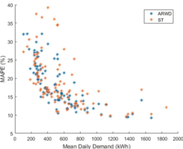
The relationship between mean daily demand (for the last year) and the errors are shown in Fig. 3 for ARWD and ST. It clearly shows the methods have smaller relative errors for the larger substations as expected.
From these results, we therefore expect the best methods to be the
ARWD, the ST and the Snt. We would also expect bigger peak reductions for larger feeders since the demands are more predictable and therefore the control can be more effective.
3.2 Peak reduction
Fig. 4 shows the boxplot for peak reduction for each control method, each forecast method and the best possible peak reduction, PR da∗ . Overall, on average all forecast methods and control techniques
achieved some peak reduction. The least increase on the peaks was achieved by ARWD. Yet, on average Snt provided best peak reduction for both fixed and MPC, closely followed by ARWD. Fig. 5 shows Snt forecast against observed demand and resultant demand with BESS schedules.
Comparison of Fig. 6 and the overall mean peak reduction in Table 1 show that there is no clear performance improvement of MPC with simple error over the fixed schedule averaged for all feeders day-wise and feeder-wise comparison in Table 2 shows that MPC with fixed error performs better than fixed schedule about half-of the time.
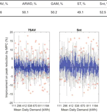
The results here confirmfirstly that the more accurate forecasting methods produce the greatest peak reduction. Secondly, we can also see there is a clear relationship between peak reduction and the mean daily demand of the feeder. As expected, due to the volatility of small feeders, in these cases the control methodologies on average actually increases the size of the peak. Fig. 7 suggests a potential relationship between improved peak reduction with MPC and mean daily demand, with smaller feeders to have better peak reduction than thefixed schedule.
4
Discussion
Comparison of MAPE for a range of feeder sizes shows that some forecast perform better for certain types of feeders. Hence, there
Fig. 3 Relationship between MAPE and mean daily energy demand for each feeder for two of the forecast methods
Fig. 4 Comparison of the daily peak reduction for each forecasting method and each scenario:PRd∗o ,PRd∗f andPRd∗m
Fig. 5 Observed, forecasted demand and profiles resulting from best possible,fixed and MPC schedules based onSntforecasting method
was no one forecast that suited all feeders. We tested a number of forecast methods against a competitive benchmark. An advantage of all methods is their simplicity and computational speed in being implemented.
Forecast accuracy is a strong driver for potential peak reduction but accuracy was driven strongly by mean daily demand on the
feeder. Hence, the effectiveness of storage is linked to the number of customers on a feeder and the size of these customers. As the result, better peak reduction was achieved with fixed schedule and MPC with simple error correction for the feeders with greater mean daily demand. For small feeders, BESS withfixed schedule actually increases the peak demands. Hence, there should be a minimum size threshold when deciding if a feeder is suitable for BESS with scheduling algorithms. However, MPC with the fixed error demand update method, performed better than fixed schedule, particularly on smaller feeders. Further investigation is required on the correlation of forecast errors and demand characteristics on smaller feeders. More sophisticated error modelling techniques (e.g. rolling forecast) are expected to improve the performance of MPC, especially on larger feeders.
In case of operational implementation of BESS on a LV distribution feeder, the control system is typically based on multiple stages: planning and real-time operation. The real-time operation control is happening at a much higher resolution than the half-hourly planning stage. The half-hourly demand represents an average power within the half-hour meaning that the actual peaks measured at the higher-resolution (e.g. 5 s or one minute) would be significantly greater that the half-hourly average.
Furthermore, this paper only considered aggregated demand across three phases at half-hourly resolution. Due to the number of customers on each phase and their individual behaviour, the demand is likely to be unbalanced. Although balancing the demand on the phases would not decrease the aggregated half-hourly demand, peaks on each phase measured at higher resolution are likely to be significantly reduced, assisting with managing the thermal constraints on the feeder.
5
Summary
The paper has presented a comparison offive forecasting techniques for prediction of LV feeders and their role in the reduction of peak demand using two energy storage control techniques: fixed schedule and model predictive control. The forecasting techniques and control algorithms have been assessed on demand data for 14 days from 100 LV feeders.
Results show that certain type of forecasts perform better for certain sizes of feeders and consequently lead to better performance of the peak reduction algorithms. Bothfixed schedule and MPC with simple error achieved better peak reduction for larger feeders. However, MPC with simple error correction have performed better on smaller feeders compared to thefixed schedule. In future work, integration of advanced demand models and rolling forecast for the model predictive control will be considered.
6
Acknowledgments
This research work was carried out as part of New Thames Valley Vision (SSET203), a LCNF project, funded by OFGEM and led by Scottish and Southern Electricity Networks.
7
References
1 Evans, G.:‘New Thames valley vision technical impact evaluation impact on DNO network from low carbon promotions’. SDRC 9.8b (SSET203), 2016
2 Joshi, K. A., Pindoriya, N. M.: ‘Day-ahead dispatch of battery energy storage system for peak load shaving and load leveling in low voltage unbalance distribution networks’. Power and Energy Society General Meeting, 2015 IEEE, 2015, pp. 1–5
3 Yang, Y., Li, H., Aichhorn, A.,et al.:‘Sizing strategy of distributed battery storage system with high penetration of photovoltaic for voltage regulation and peak load shaving’,IEEE Trans. Smart Grid, 2014,5, (2), pp. 982–991
4 Yunusov, T., Frame, D., Holderbaum, W.,et al.:‘The impact of location and type on the performance of low-voltage network connected battery energy storage systems’,Appl. Energy, 2016,165, pp. 202–213
5 Crossland, A. F., Jones, D., Wade, N. S.:‘Planning the location and rating of distributed energy storage in LV networks using a genetic algorithm with simulated annealing’,Int. J. Electri. Power Energy Syst., 2014,59, pp. 103–110 Table 2 Percentage of all days on all 100 feeders when MPC achieved
better peak reduction than fixed schedule
7SAV, % ARWD, % GAM, % ST, % Snt, %
46.6 50.1 50.2 49.1 52.5
Table 1 Overall mean peak reduction, PRdf∗ and PRdm∗
, for fixed and MPC algorithms, respectively over all feeders and days for each forecasting method
7SAV, % ARWD, % GAM, % ST, % Snt, %
fixed 2.85 5.63 2.87 5.53 5.57
MPC 2.77 5.68 3.00 5.57 6.17
Fig. 7 Percentage of days when MPC performed better thanfixed schedule in daily peak reduction for the worst and the best forecasts, 7SAV and Snt, respectively
Fig. 6 Daily peak reduction against ascending mean demand per feeder for each forecasting method based on‘MPC’scenario
6 Wade, N. S., Taylor, P. C., Lang, P. D.,et al.:‘Evaluating the benefits of an electrical energy storage system in a future smart grid’,Energy Policy, 2010,38, (11), pp. 7180–7188
7 Pezeshki, H., Wolfs, P., Member, S.,et al.:‘A model predictive approach for community battery energy storage system optimization’. PES General Meeting | Conf. and Exposition, 2014 IEEE, 2014, pp. 27–31
8 Mégel, O., Mathieu, J. L., Andersson, G.:‘Scheduling distributed energy storage units to provide multiple services under forecast error’,Int. J. Electr. Power Energy Syst., 2015,72, pp. 48–57
9 Rowe, M., Yunusov, T., Haben, S.,et al.:‘The real-time optimisation of DNO owned storage devices on the LV network for peak reduction’,Energies, 2014,
7, (6), pp. 3537–3560
10 ‘Scottish and southern energy power distribution’, 2014, New Thames Valley Vision, Available at http://www.thamesvalleyvision.co.uk/, accessed 12 June 2017 11 Haben, S., Giasemidis, G.: ‘A hybrid model of kernel density estimation and quantile regression for GEFCom2014 probabilistic load forecasting’,
Int. J. Forecast., 2016,32, pp. 1017–1022
12 Gaillard, P., Goude, Y., Nedellec, R.:‘Additive models and robust aggregation for GEFCom2014 probabilistic electric load and electricity price forecasting’,
Int. J. Forecast., 2016,32, (3), pp. 1038–1050
13 Pierrot, A., Goude, Y.:‘Short-term electricity load forecasting with generalized additive models’. Proc. of ISAP power, 2011
14 Florian, Z., Steinert, R., Husmann, S.: ‘Efficient modeling and forecasting of electricity spot prices’,Energy Econ., 2015,47, pp. 98–111