EDHEC RISK AND ASSET MANAGEMENT RESEARCH CENTRE
393-400 Promenade des Anglais, BP 3116, 06202 Nice Cedex 3 - Tel. +33 (0)4 93 18 78 24 - Fax. +33 (0)4 93 18 78 44 Email: [email protected] - Web : www.edhec-risk.com
Inflation-Hedging Properties of Real Assets and Implications
for Asset-Liability Management Decisions
No¨el Amenc
Professor of Finance at EDHEC Business School
Director of EDHEC Risk and Asset Management Research Center
Lionel Martellini
∗Professor of Finance at EDHEC Business School
Scientific Director of EDHEC Risk and Asset Management Research Center
Volker Ziemann
Senior Research Engineer
EDHEC Risk and Asset Management Research Center
Abstract
This paper presents an empirical analysis of the benefits of alternative forms of investment strategies from an asset-liability management perspective. Using a vector error correction model (VECM) that explicitly distinguishes between short-term and long-term dynamics in the joint distribution of asset returns and inflation, we identify the presence of long-term cointegration relationships be-tween the return on a typical pension fund liabilities and the return of various (traditional and) alternative asset classes. Our results suggest that real estate and commodities have particularly attractive inflation hedging properties over long-horizons, which justify their introduction in pension funds’ liability-matching portfolios. We show that novel liability-hedging investment solutions, including commodities and real estate in addition to inflation-linked securities, can be de-signed so as to decrease the cost of inflation insurance for long-horizon investors. These solutions are shown to achieve satisfactory levels of inflation hedging over the long-term at a lower cost compared to a solution solely based on TIPS or inflation swaps. Overall our results suggest that alternatives are very useful in-gredients for institutional investors facing inflation-related liability constraints.
∗Lionel Martellini is the author for correspondence. He can be reached at the following address: Edhec Risk
and Asset Management Research Center, 400 Promenade des Anglais, BP 3116, 06202 Nice Cedex 3, France; email: [email protected]. We acknowledge financial support from Morgan Stanley Investment Management, the sponsor of the Research Chair in ”Financial Engineering and Global Alternative Portfolios for Institutional Investors” at EDHEC Risk and Asset Management Research Center.
1
Introduction
A recent surge in worldwide inflation has increased the need for investors to hedge against unexpected changes in price levels. In the most recent forecasts, global con-sumer price index (CPI) inflation has been revised up more than a percentage point, to 5.0%, for calendar 2008, and by 0.7 percentage points, to 3.7%, in 2009, a trend which is likely to continue for the foreseeable future despite the current crisis, given the long-term increased demand pressure on food and energy resources. The CPI infla-tion peak has been forecasted to be 4.1% in the euro area and 5.5% in the US, and the direct impact of higher food and energy raw material costs is estimated to account for 2.5 percentage points and 3 percentage points, respectively, of these rates.1 Inflation
acceleration in emerging market countries will likely be larger than what is seen in developed countries, reflecting the much greater importance of food in their economies and their generally stronger rates of growth. As a result of these trends, inflation hedg-ing has become a concern of critical importance not only for private investors, who consider inflation as a direct threat with respect to the protection of their purchasing power, but also, and perhaps more importantly, for pension funds who face pension payments that are indexed (conditional or full indexation) with respect to consumer price or wage level indexes.
This focus on inflation hedging is consistent with the heightened focus on liability-risk management that has emerged as a consequence of the 2000-2003 pension crisis. A number of so-called “liability-driven investment” (LDI) techniques have been promoted over the past few years by a number of investment banks and asset management firms, which advocate the design of a customized liability-hedging portfolio (LHP), the sole purpose of which is to hedge away as effectively as possible the impact of unexpected changes in risk factors affecting liability values, and most notably interest rate and inflation risks. This LHP complements the traditional performance-seeking portfolio (PSP), which composition is not impacted by the presence of liabilities. Within the aforementioned LDI paradigm, a variety of cash instruments (Treasury inflation pro-tected securities, or TIPS) as well as dedicated OTC derivatives (such as inflation swaps) are typically used to tailor customized inflation exposures that are suited to each particular institutional investor liability profile. One outstanding problem, how-ever, is that such solutions generate very modest performance. In fact, real returns on inflation-protected securities, negatively impacted by the presence of a significant in-flation risk premium, are typically very low. In other words, while these solutions offer very significant risk management benefits, the lack of performance make them rather costly options for pension funds and their sponsor companies. Beside, the capacity of the inflation-linked securities market is not sufficient to meet the collective demand of institutional and private investors, while the OTC inflation derivatives market suffers from a perceived increase in counterparty risk.
In this context, it has been argued that some other asset classes, such as stocks and
1See Barclay Capital Global Outlook 2008,
nominal bonds, but also real estate or commodities, could provide useful, albeit im-perfect, inflation protection at a lower cost compared to investing in TIPS. On the one hand, equity investments appear as relatively poor inflation hedging vehicles from a short-term perspective. Empirical evidence indeed suggests that there is in fact a nega-tive relationship between expected stock returns and expected inflation (see Fama and Schwert (1977), Gultekin (1983) and Kaul (1987) among others), which is consistent with the intuition that higher inflation leads to lower economic activity, thus depressing stock returns (e.g. Fama (1981)).2 On the other hand, higher future inflation leads
to higher dividends and thus higher returns on stocks (Campbell and Shiller (1988)), and thus equity investments should offer significant inflation protection over longer horizons, a fact that has been confirmed by a number of recent empirical academic studies (Boudoukh and Richardson (1993) or Schotman and Schweitzer (2000)). This property is particularly appealing for long-term investors such as pension funds, who need to match increases in price level at the horizon, but not necessarily on a monthly basis. Obviously, different kinds of stocks offer contrasted inflation-hedging benefits, and it is in fact possible to select stocks or sectors on the basis of their ability to hedge against inflation (hedging demand), as opposed to selecting them as a function of their outperformance potential (speculative demand). For example, utilities and infrastruc-tures companies typically have revenues that are heavily correlated with inflation, and as a result they tend to provide better-than-average inflation protection. Similar in-flation hedging properties are expected for bond returns. Indeed, bond yields may be decomposed into a real yield and an expected inflation components. Since expected and realized inflation move together on the long-term (see Schotman and Schweitzer (2000)), we expect a positive long-term correlation between bond returns and changes in inflation. In the short-term, however, expected inflation may deviate from the ac-tual realized inflation, leading to low or negative correlations. There again, an investor willing and able to relax short-term constraints to focus on long-term inflation hedg-ing properties will find that investhedg-ing in nominal bonds can provide a cost-efficient alternative to (or complement to) investing in inflation-linked securities.
Moving beyond traditional investment vehicles such as stocks and bonds, recent aca-demic research has also suggested that alternative forms of investments offer attractive inflation-hedging benefits. Commodity prices, in particular, have been found to be lead-ing indicators of inflation in that they are quick to respond to economy-wide shocks
2This finding is also consistent with the so-called ”Fed model”, which is used by many investment
professionals to generate signals about the relative attractiveness of stock prices relative to bond prices. The model assumes that bonds and equities compete for space in investment portfolios; if bond yields increase, then stock yields must also rise in order to remain competitive. Thus, the Fed model relates the yield on stocks (as measured by the ratio of dividends or earnings to stock prices) to the yield on Treasury bonds and to the relative risk premium of stocks versus bonds. In the long-run, the Fed model posits that the actual yield on stocks will revert to a normal yield level given by the bond yield plus the risk premium. Historically, the rate of inflation has been a major influence on nominal bond yields. Therefore, the Fed model implies that stock yields and inflation must be highly correlated. Campbell and Vuolteenaho (2004) review stock market performance between 1927 and 2002, examining the impact of risk premiums and inflation on stock yields and find strong support for the Fed model.
to demand. Commodity prices generally are set in highly competitive auction markets and consequently tend to be more flexible than prices overall. Beside, recent inflation is heavily driven by the increase in commodity prices, in particular in the domain of agriculture, minerals and energy. Consistent with these theoretical arguments, a re-cent study by Gorton and Rouwenhorst (2006) find that, over the 1959-2004 period, commodity futures were positively correlated with inflation, unexpected inflation, and changes in expected inflation. They also find that inflation correlations tend to increase with the holding period and are larger at return intervals of 1 and 5 years than at the monthly or quarterly frequency. In the same spirit, it has also been found that commer-cial and residential real estate provide at least a partial hedge against inflation, which implies that portfolios that include real estate allow for enhanced inflation hedging benefits (see Fama and Schwert (1977), Hartzell et al. (1987) or Rubens et al. (1989)). This effect seems to be particularly significant over long-horizons. Hence, Anari and Kolari (2002) examine the long-run impact of inflation on homeowner equity by in-vestigating the relationship between house prices and the prices of non housing goods and services, rather than return series and inflation rates, and infer that house prices are a stable inflation hedge in the long-run. When it comes to securitized forms of real estate investment, the situation is less clear, even though there is evidence of a long-term connection that suggest that REITs could neutralize part of the inflation risk in the long run (Westerheide (2006)).
In order to assess the inflation hedging potential of the various asset classes within a unified framework, we follow the literature on predictability of asset returns (see e.g. Kandel and Stambaugh (1996), Campbell and Viceira (1999) and Barberis (2000)). As such, our analysis is closely related to Hoevenaars et al. (2008) who construct optimal mean-variance portfolios with respect to inflation-driven liabilities based on model-implied forward looking variances and expected returns. Their basic finding is that alternative asset classes add value to the investor’s portfolio and command significant positive allocation in the optimal mean-variance portfolio. The authors further stress that the allocations in alternative asset classes are higher within the optimal asset-liability portfolio as opposed to optimal asset-only portfolio. In what follows, we extend this existing literature in several directions. First, we note that modeling returns with a vector auto-regressive (VAR) model on log-returns, as was mostly done in previous research on the subject, omits any information on price dependencies and long-term equilibria to purely focus on short-term effects in return series. In order to address this shortcoming of the VAR model, we include cointegration relationships in the model and assess sensitivities of model-implied dynamics with respect to these additional factors that capture price dependencies in addition to return dependencies. The resulting error correction form of the vector-autoregressive model (VECM), or cointegrated VAR model, has the striking advantage, as compared to the standard VAR representation, that it explicitly distinguishes between short-term and long-term dynamics in the joint distribution of asset returns and inflation. While error correction form of the vector-autoregressive model have been extensively used in the macroeconomic literature in order to distinguish between trends and business cycles and thus between stationary
and non-stationary components in consumption and wealth dynamics (see e.g. Lettau and Ludvigson (2004) or Beaudry and Portier (2006) for recent studies), this approach is relatively new in the finance literature. It has been used in modeling price and return dependencies of financial securities (e.g. Blanco et al. (2005) or Durre and Giot (2007)) and, more recently, in inflation hedging contexts (Westerheide (2006) or Hoesli et al. (2007)).
To the best of our knowledge, our paper is the first to provide a comprehensive VECM model for the formal analysis of inflation-hedging properties of various traditional and alternative classes. We derive econometric forecasts for model-implied volatilities and correlations, and we find that the results strongly deviate from what is obtained with a standard VAR model (see Sections 3 and 4). Using the VECM model that explicitly distinguishes between short-term and long-term dynamics in the joint distribution of asset returns and inflation, we identify the presence of long-term cointegration rela-tionships between the return on a typical pension fund liabilities and the return of various (traditional and) alternative asset classes. Our results suggest that real estate and commodities have particularly attractive inflation hedging properties over long-horizons. Subsequently, we use the VECM fitted parameters in order to perform a simulation-based analysis of the impact on ALM risk budgets of various portfolio allo-cations. More precisely, the paper suggests a structural form of the model that incor-porates i.i.d. innovations, which allows for the generation of a stochastic Monte Carlo analysis in a straightforward manner. The afore-mentioned findings suggest that novel long-term liability-hedging investment solutions can be designed so as to decrease the cost of inflation insurance from the investor’s perspective. In particular, it is possible to construct enhanced versions of inflation-hedging portfolios including inflation-linked securities, but also, commodities and real estate, so as to achieve satisfactory levels of inflation hedging over the long-term at a lower cost compared to a solution solely based on inflation swaps. The intuition behind our results is rather straightforward. The in-creased expected return potential generated through the introduction of commodities and real estate in addition to TIPS in the LHP allows for a reduced global allocation to the PSP while meeting the global performance expectations, which in turn allows for better risk management properties.
The rest of this paper is organized as follows. In section 2, we present the economet-ric framework and motivate the introduction on an error correction extension of the standard VAR model. In Section 3 we describe the data base as well as preliminary statistical tests that are used for model selection purposes. In section 4, we assess the inflation hedging potential of various traditional and alternative asset classes, and con-struct different versions of enhanced liability-hedging portfolios that contain real estate and commodities in addition to TIPS. Section 5 analyzes the impact in terms of risk budget improvements of the introduction of such enhanced liability hedging portfolios. Section 6 concludes the paper.
2
Modelling return and inflation dynamics
The first key challenge that needs to be met for the analysis of the benefits of al-ternative investment strategies from an asset-liability perspective is the design of an appropriate econometric model for the joint distribution of asset returns and inflation. As recalled in the introduction, the bulk of literature on stock return predictability and return dynamics modeling (e.g. Campbell and Shiller (1988)) has relied on vector-autoregressive (VAR) models. The calibration of a VAR model is generally performed on asset return series corresponding to asset classes of interest and a set of potentially predictive economic variables that are introduced in order to enhance the explanatory power of the model. In the context of VAR models, the choice of usingreturn series as opposed toprice series is either non-motivated, or motivated by the stylized fact that return series are stationary while asset price series are not. The important consequence of stationarity follows from the Wold’s Decomposition Theorem that states that sta-tionary processes can be expressed as a moving average process (cf. Hamilton (1994, pp. 108)), which in turn allows for the derivation of analytical expressions for shock responses, expected return and forward looking variances. Secondly, non-stationarity leads to unstable, explosive and unbounded forward-looking variances and covariances, which makes the model non-tractable and non-suited for portfolio selection purposes (see L¨utkepohl (1993)). As a consequence, most econometric financial applications are based on return series or log-return series that are proven to be stationary, while price series tend to be integrated of order 1 at least. More formally, a process ytis integrated
of order d (written: yt∼I(d)) if ∆dyt is stationary while ∆d−1 is not stationary (see
L¨utkepohl (1993) for example).
One outstanding question, however, is whether taking first differences and removing information related to price dependencies is too restrictive. The main concept behind
thecointegration framework, introduced by Engle and Granger (1987), is precisely that
integrated variables may exhibit common trends that account for the non-stationary pattern in the system. Thus, linear combinations of non-stationary variables may turn out to be stationary. Formally, a process is said to be cointegrated of order (d, i) with
d, i >0, or yt∼CI(d, i), if yt is integrated of orderd (yt∼I(d)) and there exists a linear
combination β0y
t such thatβ0yt∼I(d−i). In particular, if price series are I(1), we are
interested in linear combinations of these price series that are I(0) and thus stationary. The next section introduces the error correction version of the VAR model, known as VECM model, which incorporates both leveled and differences series. In other words, the model uses systematic relationships of both cross-sectional returns dynamics and cross-sectional price dynamics.
2.1
The econometric model
Let us first consider the standard vector-autoregressive (VAR) model of order p: yt= c + A1yt−1+. . .+ Apyt−p+ ut (1)
where yt represents an×1 vector of endogenous variables, c is a constant, Ai are n×n
coefficient matrices andε is the innovation process. If the process is stable3, it may be
rewritten as a finite moving average process: yt=
t
X
k=0
Φkut−k (2)
where Φ0 is the identity matrix and the Φs are recursively given as:
Φs = s
X
j=1
Φs−jAj (3)
with Aj= 0 for allj > p.
Moreover, stability implies stationarity, meaning that expected returns, variances and covariances are time-invariant. This is a critical point for financial applications where the econometric model is used for forecasting purposes and for deriving analytical ex-pressions for expected returns, variances and correlations. In the case of non-stationary processes, variances would be unbounded and time-variant which in turn leads to un-bounded confidence intervals of the forecasted variables.
In order to infer whether a time series is stationary or not, various so-called unit root
tests are available. The most commonly used test is the Augmented Dickey-Fuller
(ADF) test (see e.g. Greene (2003)). If the test of unit roots cannot be rejected for all endogenous variables in y, the VAR process is integrated or cointegrated. As outlined above, if the variables are I(1), writing the VAR model (1) on first-differenced variables generates a stationary process:
∆yt = c + Γ1∆yt−1+. . .+ Γp∆yt−p+ ut (4)
The unfortunate consequence of using the first-differenced variables is that any informa-tion regarding price dynamics is lost, which could prove detrimental to the predictive power of the model. For example, in an early economic study on the relationship between log consumption and log income, Davidson et al. (1978) have found that infor-mation on the deviation from a long term equilibrium enhances the explanatory power of the predictive model. To account for the presence of long-term relationships in price series, the VAR model can be generalized through the following error correction form (henceforth, VECM):
∆yt = c +αzt−1+ Γ1∆yt−1+. . .+ Γp∆yt−p+ ut (5)
where z represents the deviation from the long term equilibrium. Subsequently, this rep-resentation has been used to define the cointegration framework. Indeed, if a long-term equilibrium relationship exists, it implies that z is a stationary variable. Assuming that
3A process y
tis stable if its reverse characteristic polynomial has no roots in or on the unit circle:
the long-term equilibrium can be expressed as a linear combination of the endogenous variables, we can rewrite (5) as:
∆yt= c + Πyt−1+ Γ1∆yt−1+. . .+ Γp∆yt−p + ut (6)
with the reduced rank matrix Π =αβ0. Its rankr < n determines the number of linear
independent long-term equilibrium relationships and is also called cointegration rank. In other words, there are r independent linear combinations of the lagged endogenous variables that define the cointegration relationships constitutingr stationary variables
β0y. Accordingly,αandβaren×rmatrices andβhosts the cointegrating vectors so that β0y
t is stationary and reflects the long term equilibrium relationships of the variables
while α hosts the corresponding adjustment parameters, that is, the parameters that determine the reversion speed to this long-term equilibrium. It is important to note that α and β are not unique due to the reduced rank of Π. Accordingly, additional restrictions are needed to ensure that α and β are just identified. A set of restrictions that has been accepted as a standard procedure in the econometric literature is to define the upper part of β as ther×r identity matrix. Then, it can be shown that the estimated coefficient matrices are asymptotically unbiased (see e.g. L¨utkepohl (1993, pp. 358)).Two particular cases are worth mentioning. First, ifr= 0, then there are no linear combinations of the original variables that form a stationary process, and only first-differencing may lead to a stationary system. Secondly, if r=n, yt has a stable
VAR(p) representation.
Note that we specify all entries in y as the log of the index level values. This is mainly done because economic and financial time series are often shown to have exponential trends. Writing linear regression models such as the VAR or the VECM on the log of these variables is therefore consistent with the economically assumed dynamics since taking the log of exponential process linearizes the processes. Log-returns are also convenient because they directly add up across time-intervals.
2.2
Structural model and impulse-response functions
In the context of cointegrated processes, the dynamics of the underlying variables may be separated in short-run and long-run dynamics. Short-run dynamics are driven by the structural responses to lagged innovations captured by Γi in (5). The cointegration
relationship vector β and the reversion speed vector α govern the long-run dynamics. More precisely, Π =αβ0 induces instantaneous shocks to the system if it deviates from
the long-term equilibrium. As outlined earlier, if the system is cointegrated, cross-sectional responses to shocks may be non-transitory or persistent as the time-series ”hang together”. This section introduces a modeling approach that uses long-run and short-run restrictions in order to identify the structural shocks of the system. The structural form of the model is characterized by i.i.d. innovations εt,i, as opposed to
the correlated original innovation process ut,i. For this, we search for the transformation
matrix B such that:
From the structural assumption we know that the covariance matrix of the i.i.d inno-vations ε (Σε) is diagonal. Without any loss of generality we postulate Σε to be the
identity matrix. Therefore, the original innovation covariance matrix may be written as Σu = BB0. The transformation matrix B hosts n×n parameters that need to be
identified. Since Σu is symmetric, only 12n(n+ 1) independent equations are available
from Σu= BB0. For the parameters to be just identified we need 12n(n−1) additional
restrictions. One way to do this is to use the Cholesky decomposition. Then, the contemporaneous impact matrix B is given as a lower triangular matrix. As a matter of fact, the matrix B is not unique and the ordering of the variables determines the dynamics of the structural shocks.
Given the specific context of the VECM and the fact that some shocks are persistent, we follow Breitung et al. (2004) and impose restrictions on short-run dynamics of the shocks as well as on the long-run impact matrix. According to Granger’s representation theorem (see Johansen (1995), Theorem 4.2), this matrix is given by (see Vlaar (2004) for details):
Ξ =β⊥[α0⊥(I −Γ)β⊥]−1α0⊥B (8)
with α⊥ and β⊥ such that:
α⊥0 α=β⊥0 β = 0! (9)
The rank of this matrix is n−r since r cointegrating relationships form stationary combinations, meaning thatrshocks have only transitory impacts and disappear in the long-run. As can be seen from (3), the long-run impact matrix of the structural shocks is ΞB. Straightforwardly, this matrix also has reduced rank equal ton−r. Hence, at most
rcolumns of ΞB can be zero columns since only at mostrstructural innovation can have transitory effects and at least n−r shocks must have persistent effects to the system. Given its reduced rank, each column of zeros in ΞB accounts for n−r restrictions. As shown in Gonzalo and Ng (2001), the remaining restrictions split up into r(r−1)/2 restrictions on the transitory shocks (B) and into (n−r)((n −r)−1)/2 additional restrictions on the permanent shocks (ΞB). We set the identifying restrictions through: RΞBvec(ΞB) = rl and RBvec(B) =rs (10)
while we restrict rl and rs to be vectors of zeros. The long-run restrictions may also
be written as Rlvec(B) =rl with Rl= RΞB(In⊗Ξ). The matrix B can accordingly be
estimated by the maximum likelihood method. Following Breitung et al. (2004), the corresponding log-likelihood function is given by:4
l(B) = const−T 2 log|B| 2− T 2tr ¡ (B0)−1B−1Σ u ¢ (11)
4More details on distributional assumptions and asymptotic properties of the estimation method
Once the transformation matrix is identified, we can write the Structural VECM(1) (SVECM(1)) in its reduced form:
∆yt = c + Πyt−1+ Γ∆yt−1+ Bεt (12)
This representation allows us to conduct structural impulse-response analyzes, that is, to analyze the impact of isolated independent structural shocks εt as opposed to the
correlated innovation process ut in the reduced VECM form (5). To illustrate this, we
write the model in its level variables form:
yt = c +A1yt−1+A2yt−2+ Bεt (13)
with:
A1 =In+ Γ +αβ0 and A2 =−Γ (14)
Accordingly, the VAR model structure allows us to write structural impulse-response functions as
Ξs = ΦsB (15)
with Φs as in (3). The elements in Ξs illustrate the impacts of unit structural shocks
that occurred at time t on the endogenous variables at time t+s. The kl-th element of Ξs, for instance, depicts the impact of a unit structural shock to variable l at time t
on variable k at time t+s. As a result, this analysis allows us to measure the impact of inflation shocks on the various asset classes through time and to analyze short-run inflation hedging potential, in addition to the long run dynamic analysis captured by the cointegration relations and the long-run dynamics given by Ξ∞. Confidence intervals for
impulse-response functions are computed based on the bootstrap procedure described in Br¨uggemann (2006). In other words, we can assess co- or counter-movements between the inflation index and asset returns, and subsequently analyse horizon dependent inflation hedging capacities for the various asset classes. It is further worth mentioning that the impulse response functions converge towards the long-run impact matrix ΞB. As a direct application of the structural VECM, section 5 uses the i.i.d. innovation process property in order to perform a Monte Carlo analysis based on the fitted model. The generated scenarios will be subsequently exploited in a portfolio construction con-text.
3
Data and model specification
Our empirical analysis focuses on a set of traditional and alternative asset classes. Stock returns are represented by the CRSP value-weighted stock index. Commodi-ties are proxied by the S&P Goldman Sachs Commodity index (GSCI). Real estate investments are represented by the FTSE NAREIT real estate index, which is a value-weighted basket of REITs listed on NYSE, AMEX and NASDAQ. We thus limit the opportunity set to liquid and publicly traded assets. Finally, we add the Lehman Long
US Treasury Index, as well as the one-month Treasury bill rate.5 Following the
ev-idence from the extensive literature on return predictability (see Stock and Watson (1999) among others), we also add potential predictive economic variables to the set of endogenous variables. We introduce the dividend yield (see e.g. Campbell and Shiller (1988), Hodrick (1992) or Campbell and Viceira (2002)), the credit spread (computed as the difference between Moody’s Seasoned Baa Corporate Bond Yield and the 10-Year Treasury Constant Maturity Rate), as well as the term spread (obtained from the difference between the 10-Year Treasury Constant Maturity Rate and the 1-month-T-Bill rate). The dividend yield data is obtained from CRSP and all other economic figures were obtained from The US Federal Reserve Economic Database.6 Our analysis
is based on quarterly returns from Q1 1973 through Q4 2007.
Regarding the liability side, we include an inflation proxy represented by the consumer price index (CPI). As in Hoevenaars et al. (2008), we assume that the fund is in a stationary state as would be the case in a situation where the age cohorts and the built-up pension rights per cohort are constant through time. Under this assumption, and further assuming that liability payments exhibit unconditional inflation-indexation, the return on the liability portfolio can be proxied as the return on a constant maturity zero-coupon TIPS with a maturity equal to the duration of the liability cash-flows.7 We
construct the time-series for such constant maturity zero-coupon TIPS in accordance with the methodology described in Kothari and Shanken (2004), which states that the nominal return on a real bond is given as the sum of a real yield plus realized inflation. The real yield is in turn obtained as the difference of the nominal yield and the sum of expected inflation plus the inflation risk premium. As in Kothari and Shanken (2004), we assume the inflation risk premium to be equal to zero.8 We simplify
the computation of expected inflation by taking it as the 60-months moving average inflation. As a result, we obtain the returns on liabilities as:
rL,t =yield(tτ)−Et(π) (16)
where the upper index τ indicates the duration of the liabilities, which we have arbi-trarily chosen in what follows to be equal to 20 years.9 In Appendix A.2, we provide a
detailed derivation of the pricing scheme for inflation-indexed liabilities.
5The series is downloadable from Kenneth French’s web site (borrowed from Ibbotson Associates). 6See http://research.stlouisfed.org/fred2.
7Incorporating additional features such as actuarial uncertainty and inflation indexation would not
impact the main message of the paper, which focuses on the inflation-hedging properties of real assets.
8Note, that Kothari and Shanken (2004) also considered the case of a 50bps per annum inflation
premium.
9Hoevenaars et al. (2008) use 17 years as the duration of the liability portfolio. To avoid having to
rely on interpolation, we rather use observable interest rate series from the FED, which are exclusively available for the maturities 1, 3, 5, 6, 7, 10 and 20 years (see http://research.stlouisfed.org/fred2).
3.1
Model selection
We begin our empirical analysis with a number of preliminary tests that help us select the appropriate econometric model. Table 1 presents the results of Augmented Dickey-Fuller (ADF) tests for level, differenced and twice differenced series. The results clearly show that all price series (level series) are non-stationary and thus integrated of at least order 1. The results further indicate that some economic variables are I(1), while other variables are I(2) as illustrated by the ADF tests on first and second differences. In fact, for all log asset return series as well as for the credit and term spread series, we reject the hypothesis of a unit root. The corresponding price series are therefore integrated of order 1 and denoted by I(1)-variables. Other predictive economic variables (dividend yield, 10-year yield, CPI) and the T-bill rate exhibit the pattern of I(2) variables since taking second differences of the original price series is needed to eliminate the non-stationarity in the variables.
The presence of I(2) integrated variables is a concern since it implies that the coin-tegrating relations may still exhibit unit roots. As defined in L¨utkepohl (1993), the system is said to be integrated of order 2, which we denote by yt∼I(2), since the highest
order of integration among the set of variables is 2. In order to address I(2) processes, the VECM model a priori needs to be extended to polynomial- or multi-cointegration frameworks, meaning that second differences, linear combinations of first differenced variables and linear combinations of level variables are included in the econometric model (see Johansen (1995) for more details on the methodology). Two approaches have been proposed in the econometric literature in order to circumvent the prob-lem caused by such an increase in the model complexity. A first approach consists of transforming the I(2) variable into I(1) variables without loss of information. The idea is to choose a control variable among the I(2) variables that is supposed to move homogeneously with the remaining I(2) variables. Subtracting this variable from the others transforms the variables from I(2) into I(1) variables since the common trend is eliminated. A convenient choice for the control variable in our setup is the price index since subtracting it to the series means that the remaining I(2) variables will accord-ingly be transformed from nominal to real variables. Additionally, the control variable itself, in our case the price index, needs to be replaced by its first difference. This nominal-to-real transformation has been studied in Juselius (2007) and is inspired by preceding studies such as Engsted and Haldrup (1999), who consider various settings where some variables are I(2), and show that adding their first differences as regressors to the model leads to consistent stationary expressions for the long-run equilibrium. A drawback of this approach is that it supposes price-homogeneity for the economic variables and thus a common trend in the price level and the corresponding nominal variables, a rather strong assumption that needs to be empirically justified. A second possibility to circumvent the problem of I(2) variables is to find cointegrating rela-tionships, that is, linear combinations of I(1) and I(2) variables that are stationary. Then, the system is said to be cointegrated of order (2,0), yt∼CI(2,0), meaning that
there exists a cointegration matrix β such that β0y
t∼I(0). This is also referred to
recommendations in Hansen and Juselius (1995), who argue that ex-ante cointegration rank tests should be accompanied with ex-post analysis of the cointegrating vectors. Accordingly, we will first specify the cointegration rank r and than try to findr linear combinations that form stationary variables. It is important to note that, because of the normalization in the cointegration matrix β (see section 2.1), different orderings of the variables lead to different cointegrating relationships.
Table 2 presents the results of the Johansen trace test for the cointegration rank. The results suggest that the cointegration rank is either 6 or 7. We proceed as follows: for each permutation of the order of variables, we estimate the reduced form VECM with cointegration ranks r= 6 and r= 7 and extract the time-series across the cointegrating vectors β0y
t. Next, we perform ADF unit root tests in order to test for stationarity of
the cointegrating vectors. The ”best” ordering is evaluated as the one that leads to the smallest p-values associated with the unit root tests. Tables 3-5 yield the estimation results for the ”best” specification of the model measured by stationarity analyzes on the cointegrating vectors. The p-values associated with this order of variables range from 0 to 5.98% for the 6 vectors, which are reasonably low values.
Table 4 presents information regarding the estimated cointegrating vectors. As ev-idenced by the results, all 6 equilibrium relationships are quite similar with respect to the relevant, non-normalized parameters. In fact, for each of the 6 first variables (liabilities, long bond, stocks, CPI, Yield (10Y) and T-Bills) the remaining variables enter through a similar linear equilibrium relationship. While the loading on commodi-ties and real estate is negative within the equilibrium relationship, credit spread, term spread and dividend yield enter the long-term relationship positively. Accordingly, the interpretation of the impact of the cointegrating relationship on the return dynamics merely depends on the adjustment speed parameters displayed in Table 5. The next section presents model-implied volatilities, correlations and impulse-response functions. In addition to the VECM estimates, we also estimate for comparison purposes the stan-dard VAR(1) model on quarterly returns. Indeed, our goal is to show that explicitly accounting for the presence of cointegration relationships leads to significantly differ-ent results from what is obtained from the standard benchmark VAR model used in previous literature.
3.2
Model implied variances, correlations and impulse
re-sponses
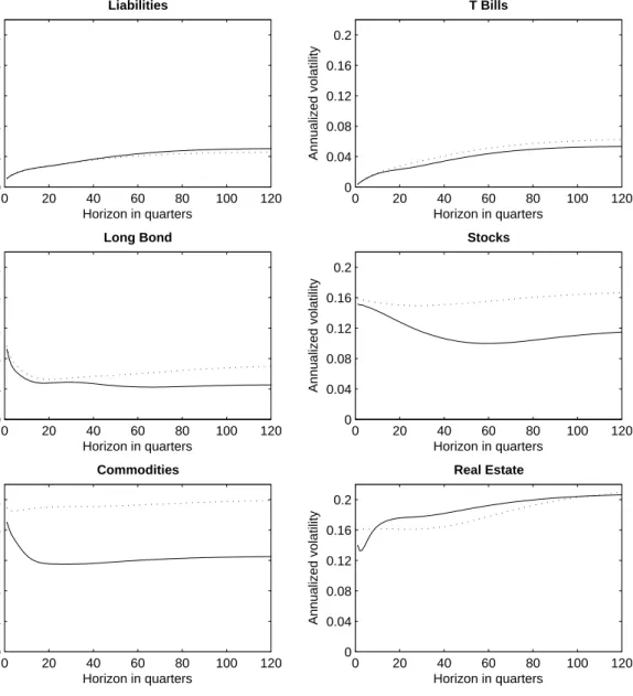
Based on the estimated structures, we derive for both the VECM and the VAR(1) model implied properties of the return dynamics. In Figure 1, we plot annualized volatilities for returns on liabilities and asset classes for different investment horizons according to the equations derived in appendix A.1. A particular focus of the graphs is on the difference between VAR-implied volatilities (dashed lines) and VECM-implied volatilities (solid lines). The differences between the two econometric methodologies turns out to be rather significant for bonds, stocks and commodities, with
VECM-implied volatilities proving to be significantly lower than VAR-VECM-implied volatilities for these classes. Liability, T-bill and real estate returns do only show minor differences between the VAR and the VECM approaches. The difference in implied volatility estimates is due to the equilibrium reverting character of the additional part αβ0y
t−1.
As explained above, whileβ0y
t−1 establishes the equilibrium relationship, αdetermines
the instantaneous impact of a deviation from this equilibrium on ∆yt. In an attempt to
shed some light into this discrepancy between VAR and VECM implied characteristics for stocks and commodities, it is worthwhile to refer to the credit spread variable. First, credit spread is highly significant as a predictive variable for both stocks and commodities. Secondly, credit spread enters positively into all cointegrating vectors with t-statistics ranging between 8 and 10. Given that stocks (respectively, commodity) returns depend positively (respectively, negatively) on changes in credit spread (see Table 3) and given that (according to Table 5) the highest adjustment parameter values are negative (respectively, positive) the long-term dynamics partly offsets the short-term dynamics, which in turns reduces the volatility. For real estate and liabilities, this offsetting effect is less pronounced, as evidenced by the balanced set of adjustment parameters in Table 5, meaning that some are positive while other are negative, which eventually cancels much of the overall long-term impact on the corresponding return dynamics.
A second remarkable effect is that VAR-implied volatilities seem to indicate that as-sets become more risky as the investment horizon increases, while VECM volatilities have contrasted implications for the various assets. Liabilities, T-bills and real estate investments appear to be more risky in the long run, while bonds, stocks and com-modities exhibit a downward sloping volatility structure, especially from very short to medium-term horizons. It should be noted at this stage that a mean-reversion effect is already present in the VAR model, and is due to a mean-reversion effect induced by the predictive power of specific lagged variables and negative relationships for in-stantaneous covariances, as explained in Campbell and Viceira (2005). For instance, stock returns exhibit some evidence of predictability through lagged dividend yields as evidenced by positive coefficients in Tables 3 and 9. At the same time, contem-poraneous innovations are negatively correlated (see Table 6). As a result a positive shock in t on dividend yields goes (on average) along with a negative shock on stock returns in t and, through the autoregressive link, a positive shock on stock returns in
t+1. The offsetting effect may be interpreted as mean-reversion, which in turn lowers the volatility of compounded stock returns. However, our findings suggest that this predictability-induced mean-reversion effect is small compared to the mean-reversion effect induced by the long-term co-integration relationships.10
Next, Figure 2 displays horizon-dependent correlation coefficients between liability re-turns and the return on various asset classes. The plots clearly suggest that bond, stock
10It should be noted that Campbell and Viceira (2005) have found with a VAR model a steeper
downward sloping volatility term structure for stock returns, but their analysis is based on real return series, while we explicitly analyze on the one hand the nominal returns, and its inflation component on the other hand.
and real estate returns are negatively correlated with liabilities in the short run, and that the correlation coefficient exhibits an upward pattern as the investment horizon increases. Bond returns and stock returns start to become positively correlated with liability returns after about 60 quarters (15 years) and end up with a significant positive correlation of roughly 0.4 with a 30-year investment horizon. Again, the result allows us to identify significant discrepancies between VAR and VECM models, especially for commodities and real estate. Commodity returns are positively correlated with liabil-ity returns in both cases, but the VECM implies a significantly higher and more stable correlation than the VAR. Model-implied correlations between real estate and liability returns, on the contrary, are significantly higher in the VAR model when compared to the VECM. This may be due to the fact that commodities are part of all 6 long term equilibrium relationships, a result of the normalization process of the matrix β and the variable order permutation procedure described above. The next section evaluates the impact of these model-implied moments and co-moments from a liability hedging portfolio perspective.
Impulse-response functions (Figure 3) indicate that with the mere exception of com-modities all responses to a structural liability shock are higher when implied by the VECM. This is mainly intrinsic to the model as by definition some shocks are persistent which can not be the case in VAR model-implied shocks, an important restriction of the latter class of models.
4
Inflation hedging properties of various assets and
portfolios
Investment horizon dependent allocation decisions have been widely studied in the liter-ature over the last decade. Brandt (2005) and Campbell and Viceira (2005) discuss the differences between short-term or myopic and intertemporal asset allocation decisions. The term structure of risk, merely driven by the presence of mean-reversion effects, with different speeds of mean reversion (see Lettau and Wachter (2007)), also plays a central role in asset allocation decisions in the presence of liabilities (see also Campbell and Viceira (2005) for the notion of term structure of risk). This section uses VECM model-implied dynamics in order to assess inflation hedging potential across different investment horizons.
Consistent with the portfolio separation theorem, we will study the liability hedging portfolio (LHP) separately from the performance seeking portfolio (PSP). In a frame-work where liabilities are indexed with respect to inflation, and when short-term liabil-ity risk hedging is the sole focus, the optimal LHP allocation consists of investing 100% into the inflation-indexed bond portfolio (TIPS portfolio), which unfortunately leads to very limited upside potential. Consequently, the investor needs a relatively sizable significant allocation to the PSP in order to meet the return requirements, which in turn generates a relatively high funding risk. Intuitively one would expect that
re-laxing the constraint of a perfect liability fit for the LHP at the short-term horizon would allow one to include alternative asset classes in the LHP, which in turns leads to an increased upside potential. Overall, this would allow an investor to reduce his/her allocation in the PSP, which in turn shall lead to a reduced surplus risk. To formalize this intuition, we perform a scenario-based analysis in order to derive the funding ratio distribution at various investment horizons. The data generating process is described by the vector error correction model (VECM) introduced in section 2.1. We further use the structural model so as to disentangle the correlated innovation process and trans-form it into i.i.d. innovations. We draw i.i.d. random variables from the multivariate standard normal distribution for the structural innovationsεs
t (s= 1. . . S) and obtain
the modeled returns by:
∆yts = c + Πyts−1+ Γ∆yts−1+ Bεst (17) for a total of S= 5,000 simulated paths. The first variable in ys
t represents the
lia-bility return. We evaluate the different portfolios in terms of the funding ratio (FR) distribution. The funding ratio att in scenarioss is accordingly given by:
FRs
t = exp ((ω0−ι)yst) (18)
whereιdenotes then×1 vector containing a 1 in the first position and zeros elsewhere, and ω is the portfolio vector. We first analyze the potential of stand-alone inflation hedging portfolios before constructing optimal portfolios.
4.1
Stand-alone hedging potential
This section assesses the inflation hedging potential of the various asset classes on a stand-alone basis. The analysis follows the methodology previously described, that is, all conclusions are drawn from the funding ratio distributions over the 5,000 simulated scenarios based on the fitted VECM dynamics (cf. previous section). We compare in-vestments in the perfect liability hedging portfolio (TIPS) to inin-vestments in traditional assets (bonds and stocks) and to investments in alternative investments (commodities and real estate). Various investment horizons from 3 through 30 years are considered. Table 10 presents the relevant indicators for the funding ratios assuming a 100% in-vestment in the corresponding traditional or alternative asset class. The first column of the table refers to the liability hedging portfolio that is obtained by a 100% invest-ment in an inflation-indexed security that has the same maturity as the liabilities.11 In
this simplified setting, this 100% TIPS liability hedging portfolio in fact proves to be
11Note, that in reality such portfolios may be unavailable as TIPS are issued for a small number
of maturities. For instance, in the US, only TIPS with maturity up to 10 years are available. Note further that we omitted statistics for T-Bill portfolios from these tables. In fact, even though T-Bills are well correlated with the liability returns, they exhibit a significant lack of relative performance due to the term spread risk premia contained in the liability return. As a result, T-Bills under-perform liabilities significantly and are not a natural candidate for the liability-hedging portfolio.
a perfect match for the liability, and therefore mean funding ratio are equal to 1 with a 100% probability for all time-horizons.12 The mean funding ratios for other classes
in Panel A are higher than 1, which indicates that all assets have, on average, higher returns than the liability stream. This is consistent with the observed historical values that have been used to calibrate the data generating process described in the previ-ous section. On the other hand, these asset classes involve the introduction of some liability risk, as evidenced by the number in Panel B and Panel C. The shortfall prob-abilities in Panel B illustrate the time-horizon characteristics of the assets with respect to the liabilities. Indeed, shortfall probabilities systematically decrease as the invest-ment horizon increases. This is consistent with results obtained for the model-implied volatilities and correlations with the liabilities (see Figures 1 and 2). The correlation between bonds, stocks and real estate with the liabilities increases with time-horizon. Additionally, volatilities decrease with the investment horizon for bonds, stocks and commodities, and slightly increase, in relative terms, for real estate, while the model-implied volatilities of liability returns sharply rise as the investment horizon increases. Furthermore, the superior returns of the assets explain a part of the observed down-wards sloping shortfall probabilities since they translate into a steeper positive trend in the numerator than in the denominator of the funding ratio. The strong decrease in shortfall probability for stocks is also explained by the structural relationship between liability shocks and aggregated responses to stock returns (see figure 3). Indeed, the persistence of liability shocks is much more pronounced for stocks than for other assets. As far as commodities are concerned, the response to liability shocks is immediate but not persistent which explains why shortfall probabilities decrease less sharply than in the case of stocks. Real estate on the other hand reacts negatively in the short run but ”recovers” as the liability shocks leads to persistently positive shocks to future real estate returns.
Overall, these shortfall probabilities are quite high in the short run, with numbers ranging from 37% (stocks and real estate) to 47% (long bond) and fall, at least for stocks and real estate, which suggest that moving away from TIPS, if it allows for a better performance (mean funding ratios greater than 1), involves significant short-term liability risk. On the other hand, these values eventually decrease in the long-run for stocks and real estate (with shortfall probabilities equal to 10% and 15%, respectively), while they remain at a high level for commodities (25%) and the long bond (38%). In Panel C we present the probabilities that the asset portfolio value falls ”severely” short of the liability portfolio value.13 For short investment horizons, these severe
or extreme shortfall probabilities are alarmingly high with numbers higher than 20%. Additionally, for the long bond, extreme shortfall probabilities do not seem to decrease in the long run (26% for 3 and for 30 years with even higher numbers in the mid-run).
12In practice, the presence of non-financial sources of risk, e.g., actuarial risk, implies that there is
some remaining funding risk even with a solution invested 100% in inflation-hedging instruments with maturities matching the maturity dates of the pension payments.
13Throughout this study, severe shortfalls are defined as a situation with a funding ratio is lower
As far as commodities are concerned, one obtains a modest decrease from 26% (3-7 years) to 20% (30 years). On the other hand, stocks and real estate exhibit similar significantly downwards sloping patterns as in the case of shortfall probabilities (Panel B). Across all 4 assets, we observe that the level of severe shortfall probabilities (Panel C) is only slightly below the level of standard shortfall probabilities (Panel B) which, obviously, is a great concern for the pension fund.
As a first result, we find that both commodities and real estate exhibit potentially interesting features in an asset liability management context. Both largely outperform the liability on average, and exhibit inflation-hedging potentials that increase in the long-run. In fact real estate exhibits shortfall probability figures that are as competitive as stocks and that sharply decrease with the investment horizon (from 37% for 3 years to 15% for 30 years). Commodities substantially outperform bonds in terms of average funding ratio and shortfall probabilities. Based on these encouraging results, we expect significant gains from adding commodities and real estate to the pure liability hedging portfolio invested in TIPS.
4.2
Liability hedging portfolios
The results from the previous section seem to suggest that introducing commodities and real estate, in addition to TIPS, in a pension fund LHP would allow for upside-potential while limiting shortfall probabilities to a reasonably low level, at least from a long-term perspective. In what follows, we quantify the trade-off between a deviation from the perfect liability match and the resulting return upside potential, which in turn will have the welcome side effect of decreasing the required contributions. The consequences in terms of ALM risk budgets of introducing alternative asset classes so as to design enhanced liability-hedging portfolios with improved performance will be quantitatively analyzed in section 5.
In order to analyze the characteristics of liability hedging portfolios that are enhanced by commodities and real estate assets, we proceed in two steps. First, we find the optimal portfolio mix of commodities and real estate and secondly, this portfolio is added to TIPS in various proportions so as to form the enhanced liability hedging portfolio (henceforth enhanced LHP). The first step is addressed by finding the portfolio of commodities and real estate that minimizes the tracking error volatility with the TIPS portfolio. Figure 4 shows the resulting portfolios as a function of the investment horizon. As evidenced by the graph, the portfolio is well-balanced between the two assets, and the position in commodities increases with the investment horizon.
Table 11 presents funding ratio statistics for the enhanced LHP. Various portfolios, ranging from 0% to 50% of alternative investments (AI) with the remainder in TIPS, are studied. The mean funding ratio of the enhanced LHP is a simple linear combination of the individual mean funding ratios and the interpretation is straightforward. In particular, Panel A of table 11 shows that the upside potential is an increasing function of the percentage allocated to alternative assets within the LHP portfolio. On the
other hand, the more the investor allocates to the alternative assets, the higher is the risk to fall severely short of the liabilities. However, the results suggest very important gains when stepping from stand-alone alternative asset classes to alternative investment portfolios in terms of shortfall probabilities. Indeed, at all investment horizons, the shortfall probabilities are significantly lower for various versions of the enhanced LHP compared to the results obtained for the stand-alone assets (Table 10). For instance, for investment horizons of 10 years (respectively, 20 years), shortfall probabilities are as low as 17% (respectively, 9%) compared to 27%-35% (respectively, 19%-29%) on the stand-alone basis.14 More importantly perhaps, Panel C indicates that the decrease
in severe shortfall probability is substantial. Even for a rather important investment to the AI portfolio of 50%, severe shortfall probabilities are only 6% in the short-run and 2% for long investment horizons. For modest investments to the AI portfolio (0%-15%), the severe shortfall probability even decreases to 0% meaning that none of the 5,000 simulated paths yields a funding ratio lower than 90%, whatever the investment horizon. Overall these results suggest that the introduction of alternative investment vehicles may lead to increased upside potential for the LHP without severely increasing the shortfall risk.
5
Implication for risk budgeting in asset-liability
management
This section attempts to study the impact of the introduction of real estate and com-modities within the liability-hedging portfolio on the level of expected funding ratio over various time-horizons.
5.1
Risk budgeting with LDI solutions
In terms of risk budgets, the implementation of LDI solutions critically depends on the attitude towards risk. It is typically understood that high risk aversion levels leads to a predominant investment in the liability-hedging portfolio, which in turn implies low extreme funding risk (zero risk in complete market case), as well as low expected performance and therefore high necessary contributions. On the other hand, low risk aversion levels lead to a predominant investment in the performance-seeking portfolio, which implies high funding risk as well as higher expected performance, and hence lower contributions. To formalize this intuition, one may compare the initial contribution that is needed to generate a 100% funding ratio at the horizon when the investor’s portfolio is fully invested in TIPS (the perfect liability-hedging portfolio) versus the initial contribution needed to generate an average 100% funding ratio at
14Note that shortfall probabilities solely depend on the investment horizon and not on the fraction
allocated to the AI portfolio. This result is intrinsic to the buy-and-hold methodology and the fact that the TIPS portfolio exhibits non-stochastic funding ratios equal to 1.
the horizon when risky asset classes such as stocks and bonds are introduced. Figure 6 presents a graphical representation of this effect for different investment horizons. For instance, for an investment horizon of 20 years, an allocation of 40% to the PSP (which is so far assumed to contain stocks and bonds in a proportion that generates the maximum Sharpe ratio - see Figure 5) and 60% in the liability hedging portfolio fully invested in TIPS allows one to reduce the initial contributions by almost 20% compared to a 100% investment in TIPS liability-hedging portfolio. Of course, this contribution saving effect comes at the cost of introducing funding risk at the global portfolio level. As can be seen from Panel B in Table 12, shortfall probabilities show a significant increase in the allocation to the PSP, even though it should be noted that the magnitude of this effect decreases with time-horizon.
5.2
Improving ALM risk budgets through the introduction of
real estate and commodities within the LHP
We now analyze the impact on ALM risk budgets of the introduction of real estate and commodities within the LHP. We first draw a comparison between the option that consists of investing 100% in the LHP but enhancing the LHP with the introduction of real estate and commodities, and the option that consists in leaving the LHP fully invested in TIPS and seeking to add performance potential through the introduction of the PSP, as discussed in the previous sub-section. A comparison of the results in Panels B and C of Table 11 and the results in Panels B and C of Table 12 clearly indicates that introducing alternatives within the LHP (option 1) systematically leads to a lower increase in risk indicators compared to the introduction of traditional asset classes through the PSP (option 2). For example the probability of a shortfall greater than 90% at the 20 years horizon is 2.1% when the investor’s portfolio is invested 60% in TIPS and 40% in the combination of real estate and commodities that allows for the best liability-hedge (see Panel C of Table 11), while it reaches 5.92% when the investor’s portfolio is invested 60% in TIPS and 40% in the combination of stocks and bonds that allows for the maximum Sharpe ratio (see Panel C of Table 12).
In the same spirit, Figure 7 shows the relative contribution savings as a function of the alloation to the PSP when the LHP is enhanced by 10% alternative investments. In comparison to Figure 6, the graph suggests that for comparable allocations to the PSP, contribution savings are larger in magnitude when using enhanced LHP instead of the sole TIPS LHP. Consequently, the target contribution saving can now be reached with a lower allocation to the PSP portfolio. Figures 8 and 9 illustrate this effect for LHPs that are enhanced by the introduction of 5%, respectively 10%, of alternative investments (represented again by the portfolio of real estate and commodities that minimizes the tracking error with respect to the liability portfolio). For instance, with an LHP that is composed of 90% TIPS and 10% alternative assets (Figure 9), an allocation of only 27% to the PSP leads to the same mean funding ratio, or, equivalently, to the same contribution savings, than an investment of 40% in the PSP when the LHP is solely invested in TIPS.
Table 13 presents the corresponding ALM risk indicators , with numbers that can be compared to the results in Table 12. We observe that (for a given allocation to the PSP) enhanced LHPs do not only lead to higher mean funding ratios, but they also lead to lower shortfall probabilities (see Panel B of Table 13) compared to the case of the non-enhanced (i.e., pure TIPS) LHP (Panel B of Table 12). This is obviously related to portfolio diversification effects between traditional assets within the PSP and alternative assets within the LHP. Severe shortfall probabilities (see Panel C of Table 13) also decrease substantially when compared to the case where the LHP was represented by the TIPS portfolio (see Panel B of Table 12).
Figure 10 combines the risk and return perspectives by plotting the reduction in the probability of a deficit and probability of a severe deficit indicators when shifting from the standard LHP (100% TIPS) to the enhanced LHP while maintaining the same level of mean funding ratio. In this analysis, we consider a base case of 40% invest-ment to the PSP and 60% to TIPS, and shows the reduction of the required PSP allocation obtained by an investor willing to substitute the enhanced LHP (when ei-ther 5% alternative investments or 10% alternative investments are introduced) to the pure 100% TIPS LHP. For instance, we find that when the investment horizon is 20 years, enhancing the LHP by the introduction of 5% (respectively 10%) of the real estate + commodities portfolio allows one to reduce the allocation to the PSP by 14% (respectively, 31%) while maintaining the mean funding ratio at the same level as with the non-enhanced LHP. The graphs further shows the resulting percentage reduction in shortfall probability and expected shortfall. Again for an investment horizon of 20 years, the introduction of 5% (respectively 10%) of alternatives (real estate and com-modities) within the LHP leads to a 19% (respectively, 39%) reduction in shortfall probability. The reduction in severe shortfall probability is even greater and reaches a spectacular 42% (respectively, 78%).
6
Conclusions and directions for future research
Based on a suitable econometric framework, we have studied the relationship between inflation-driven liabilities and asset returns on bonds, stocks, commodities and real estate at various horizons. We have used the error correction form of the vector au-toregressive model (VEC model or VECM) that allows for incorporating price and return dependencies, as opposed to the standard form of VAR models that solely fo-cuses on the dynamics of returns. As a result, long-term dependencies between asset and liability values may be better captured, based on a larger fraction of the informa-tion contained in the data. We have used the VEC model-implied return dynamics in order to construct horizon-dependant volatilities and asset-liability correlations. Our empirical analysis suggests that explicitly accounting for long-term cointegration re-lationships leads to significant differences in forecasted properties of asset returns in terms of their term structure of risk and correlations with the liabilities. In particular we have found that VECM-implied volatilities are significantly lower than VAR-implied
volatilities for stocks, bonds and commodities, an effect with particularly pronounced in the long-term. This is due to the fact that mean-reverting properties of asset re-turns are accounted in a more satisfactorily manner when the econometric procedure explicitly allows for the modeling of long-term dependencies between asset returns and predictive state variables. We have also found that VECM-implied correlations between asset returns and liability returns to be significantly different from the VAR-implied correlations. In particular the liability-hedging potential of commodities seems to be understated by the VAR estimation procedure compared to the case when the presence of long-term cointegration relationships is explicitly accounted for.
We have used the structural form of the VEC model to perform a Monte Carlo simula-tion exercise and generate a large number of simulated scenarios for asset and liability returns in order to analyze the distribution of funding ratios of various portfolios at different time-horizons. We have found that various alternative asset classes exhibit attractive inflation-driven liability hedging properties. For instance, investing in com-modities leads to very low shortfall probabilities at virtually all investment horizons. While investing in real estate leads to higher shortfall probabilities in the short and medium run, significantly lower probabilities are obtained in the very long run (>30 years). These results suggest that novel liability-hedging investment solutions, in-cluding commodities and real estate in addition to inflation-linked securities, can be designed so as to decrease the cost of inflation insurance for long-horizon investors. These solutions are shown to achieve satisfactory levels of inflation hedging over the long-term at a lower cost compared to a solution solely based on TIPS or inflation swaps. The increased expected return potential generated through the introduction of commodities and real estate in addition to TIPS in the LHP allows for a reduced global allocation to the PSP while meeting the global performance expectations, which in turn allows for better risk management properties. For example, in the case of a 20 years investment horizon, the introduction of 5% (respectively 10%) of alternatives (real estate and commodities) within the LHP is found to lead to a 19% (respectively, 39%) reduction in shortfall probability. The reduction in severe shortfall probability is even greater and reaches a spectacular 42% (respectively, 78%). Overall our results suggest that alternatives are very useful ingredients for institutional investors facing inflation-related liability constraints.
Our analysis of the benefits of alternatives in institutional portfolios can be extended in several directions, and in particular would ideally encompass other forms of alternative investments. While we have focused on real estate, commodities, institutional investors have recently shown an increasing interest in other alternatives such as private equity and infrastructures, for which the intuition suggests that attractive inflation-hedging properties could also be obtained. The unavailability of time-series for these asset classes with the sufficient length and frequency is, however, a serious concern from the econometric perspective. One possible solution would involve the construction of liquid proxies for the returns on these assets based on publicly traded instruments with similar characteristics, but the adequacy between the proxy and the actual form of investment under consideration (private equity or infrastructure) would have to be
carefully assessed. Other alternative forms of investment that have gained popularity in institutional portfolios are external hedge funds portfolios, and also internal Global Tactical Asset Allocation (GTAA) strategies. While hedge funds and GTAA strategies are not expected to exhibit particularly attractive inflation-hedging properties, they appear as natural candidates to enter the performance-seeking portfolios because of their focus on factor-neutral alpha generation. Here again data availability is a serious concern since we do not have access to a time-series that would represent the perfor-mance of an index of typical GTAA managers, and given that return data on hedge fund managers have a rather limited history.