Adaptive Learning: Algorithms and Complexity

ADAPTIVE LEARNING:

ALGORITHMS AND COMPLEXITY

A Dissertation

Presented to the Faculty of the Graduate School of Cornell University

in Partial Fulfillment of the Requirements for the Degree of Doctor of Philosophy

by

Dylan James Foster May 2019

c

2019 Dylan James Foster ALL RIGHTS RESERVED

ADAPTIVE LEARNING: ALGORITHMS AND COMPLEXITY

Dylan James Foster, Ph.D. Cornell University 2019

Recent empirical success in machine learning has led to major breakthroughs in application domains including computer vision, robotics, and natural language processing. There is a chasm between theory and practice here. Many of the most impressive practical advances in learning rely heavily on parameter tuning and domain-specific heuristics, and the development effort required to deploy these methods in new domains places a great burden on practitioners. On the other hand, mathematical theory of learning has excelled at producing broadly applicable algorithmic principles (stochastic gradient methods, boosting, SVMs), but tends to lag behind in state-of-the-art performance, and may miss out on practitioners’ intuition. Can we distill our collective knowledge of “what works” into learning procedures that are general-purpose, yet readily adapt to problem structure in new domains?

We propose to bridge the gap and get the best of both worlds throughadaptive learning: Learning procedures that go beyond the worst case and automatically exploit favorable properties of real-world instances to get improved performance.

The aim of this thesis is to develop adaptive algorithms and investigate their limits, and to do so in the face of real-world considerations such as computation, interactivity, and robustness. In more detail, we:

1. introduce formalism to evaluate and assert optimality of adaptive learning proce-dures.

2. develop tools to prove fundamental limits on adaptivity.

3. provide efficient and adaptive algorithms to achieve these limits.

In classical statistical decision theory, learning procedures are evaluated by their worst-case performance (e.g., prediction accuracy) across all problem instances. Adaptive learning evaluates performance not just worst case, but in thebest caseand in between. This ne-cessitates the development of new statistical and information-theoretic ideas to provide instance-dependent performance guarantees, as well as new algorithmic and computa-tional principles to derive efficient and adaptive algorithms.

The first major contribution this thesis makes concerns sequential prediction, or online learning. We prove the equivalence of adaptive algorithms, probabilistic objects called martingale inequalities, and geometric objects called Burkholder functions. We leverage the equivalence to provide:

1. a theory of learnability for adaptive online learning.

2. a unified algorithm design principle for adaptive online learning.

The equivalence extends the classical Vapnik-Chervonenkis theory of (worst-case) statisti-cal learning to adaptive online learning. It allows us to derive new learning procedures that efficiently adapt to problem structure, and serves as our starting point for investigating adaptivity in real-world settings.

In many modern applications, we are faced with data that may be streaming, non-i.i.d., or simply too large to fit in memory. In others, we may interact with and influence the data generating process through sequential decisions. Developing adaptive algorithms for these challenges leads to fascinating new questions. Must we sacrifice adaptivity to process and make predictions from data as it arrives in a stream? Can we adapt while balancing exploration and exploitation?

• We introduce a notion of “sufficient statistics” for online learning and show that this definition leads to adaptive algorithms with low memory requirements.

• We develop large scale optimization algorithms for learning that adapt to problem structure via automatic parameter tuning, and characterize their limits.

• We give adaptive algorithms for interactive learning/sequential decision making in contextual bandits, a simple reinforcement learning setting. Our main result here is a newmargin theoryparalleling that of classical statistical learning.

• We provide robust sequential prediction algorithms that obtain optimal instance dependent performance guarantees for statistical learning, yet makeno assumptions on the data generating process. We then characterize their limits.

• We design algorithms that adapt to model misspecification in the ubiquitous statisti-cal task of logistic regression. Here we give a new improper learning algorithm that attains a doubly-exponential improvement over sample complexity lower bounds for proper learning. This resolves a COLT open problem of McMahan and Streeter (2012), as well as two open problems related to adaptivity in bandit multiclass classification (Abernethy and Rakhlin,2009) and online boosting (Beygelzimer et al.,2015).

BIOGRAPHICAL SKETCH

Dylan Foster was born in Phoenix, Arizona in 1992. He obtained his B.S. and M.S. in electrical engineering from the University of Southern California in 2014, and began his Ph.D. in computer science at Cornell University under the supervision of Karthik Sridharan the same year. While at Cornell, he was a recipient of the NDSEG Ph.D. fellowship, Facebook Ph.D. fellowship, and Best Student Paper Award at COLT 2018. After graduating from Cornell, he will join the Massachusetts Institute of Technology as a postdoctoral researcher at the MIT Institute for Foundations of Data Science.

ACKNOWLEDGEMENTS

Karthik Sridharan has been everything I could ask for as an advisor, and has been in-strumental in molding me into who I am as a researcher, influencing both how I choose problems and how I attack them. His relentless creativity and passion for deep and funda-mental problems is truly inspiring, and I am fortunate to have spent the last four years working with him and learning from him. Karthik has been extremely generous with his time throughout my PhD and is always eager to explain new concepts. This was invaluable early on when I was making the switch into theoretical research. Beyond this, Karthik is thoughtful, kind, and easy-going.

I have worked with many outstanding collaborators over the last four years. In roughly chronological order: Karthik, Sasha Rakhlin, Daniel Reichman, Zhiyuan Li, Thodoris Lyk-ouris, ´Eva Tardos, Satyen Kale, Mehryar Mohri, Peter Bartlett, Matus Telgarsky, Haipeng Luo, Alekh Agarwal, Miro Dud´ık, Rob Schapire, Ayush Sekhari, and Akshay Krishna-murthy. I am grateful to all of them for their patience, encouragement, and friendship. The contents of this thesis have benefited especially from long term collaborations with Sasha, Satyen, Mehryar, Haipeng and Akshay.

My committee members, Bobby Kleinberg, ´Eva Tardos, and Kilian Weinberger, were great sources of advice throughout my PhD.

I had three productive internships over the course of my PhD. These contributed in part to key results in this thesis.

First, I thank Sanjiv Kumar for hosting me in his group at Google Research NYC in summer 2016, which led to my collaboration with Satyen and Mehryar. I had a great time talking to the other researchers and visitors in the group, including Elad Hazan, Corinna Cortes, Mario Lucic, Bo Dai, Felix Yu, and Dan Holtmann-Rice.

Second, I thank Rob Schapire and Miro Dud´ık for hosting me at Microsoft Research NYC in summer 2017. While there, I had the fortunate to collaborate with Akshay

Krish-namurthy, Alekh Agarwal, and Haipeng Luo, and I enjoyed the company of the broader MSR machine learning crew, including John Langford, Hal Daume III, and the other ML interns: Christoph Dann, Hoang Le, Alberto Bietti.

Third, I thank Vasilis Syrgkanis for hosting me at Microsoft Research New England in summer 2018. Vasilis is an amazing collaborator with endless energy. I also enjoyed chatting with Nishanth Dikkala, Mert Demirer, Nilesh Tripuraneni, Khashayar Khosravi, Lester Mackey, Greg Lewis, Nika Haghtalab, Ohad Shamir, Adam Kalai, and Jennifer Chayes.

I had the fortune to spend spring of 2017 at the Simons Institute at UC Berkeley for their Foundations of Machine Learning program. Beyond the content of the program itself, I fondly remember all the late night runs to La Burrita and Top Dog with Matus and Andrej.

The students in the Computer Science department at Cornell have been great com-pany. While there are far too many to list, I have particularly enjoyed hanging out with Jonathan Shi, Rediet Abebe, Jack Hessel, Ayush Sekhari, and Eric Lee, and Stephen Mc-dowell. I thank all the members of the theory lab, including Jonathan Shi, Sam Hopkins, Rediet Abebe, Thodoris Lykouris, Rad Niazadeh, Pooya Jalaly, Hedyeh Beyhaghi, Manish Raghavan, Yang Yuan, Ayush Sekhari, Michael Roberts, and Ramhtin Rotabi.

I had great housemates throughout my time in Ithaca. Stephen, Sean, Eric, and Ayush: Thank you all for reminding me to goof off once in a while.

Finally, I thank my family: My parents Kim and Susan Foster and my sister Jamie. None of this would have been possible without their constant support and encouragement.

TABLE OF CONTENTS

Biographical Sketch . . . iii

Dedication . . . iv

Acknowledgements . . . v

Table of Contents . . . vii

List of Figures . . . x

List of Tables . . . xi

I

Overview

1

1.2 The Adaptive Minimax Principle . . . 9

1.3 Adaptive Learning for Real-World Challenges . . . 12

1.4 Organization . . . 17

1.5 Highlight: Achievability and Algorithm Design . . . 19

1.6 Bibliographic Notes . . . 23

1.7 Notation . . . 24

2 Learning Models and Adaptive Minimax Framework 28 2.1 Adaptive Minimax Value. . . 28

2.2 Statistical Learning . . . 30

2.3 Online Supervised Learning . . . 32

2.4 Online Convex Optimization . . . 34

2.5 Contextual Bandits . . . 36

2.6 The Minimax Theorem . . . 37

2.7 Chapter Notes . . . 38

II

Equivalence of Prediction, Martingales, and Geometry

39

4.2 Emergence of Martingales . . . 45

4.3 Generalized Martingale Inequalities . . . 46

4.4 The Burkholder Method . . . 47

4.5 The Burkholder Algorithm . . . 50

4.6 Burkholder Function for Matrix Prediction . . . 53

4.7 Discussion . . . 58

5 Generalized Burkholder Method and Sufficient Statistics 61

5.1 Background . . . 62

5.2 Problem Setup and Sufficient Statistics . . . 63

5.3 Burkholder Method for Sufficient Statistics . . . 66

5.4 Generalized Burkholder Algorithm . . . 70

5.5 Examples . . . 72

5.6 Time-Dependent Burkholder Functions . . . 77

5.7 Necessary Conditions. . . 80

5.8 Discussion . . . 83

5.9 Additional Results . . . 85

5.10 Detailed Proofs . . . 94

5.11 Chapter Notes . . . 107

6 Bounding the Minimax Value: Probabilistic Toolkit 108 6.1 Background . . . 109

6.2 Adaptive Rates and Achievability: General Setup . . . 113

6.3 Probabilistic Tools . . . 114

6.4 Achievable Rates . . . 118

6.5 Detailed Proofs . . . 122

6.6 Chapter Notes . . . 137

III

New Guarantees for Adaptive Learning

138

8.2 Preliminaries. . . 145

8.3 Burkholder Method and Zig-Zag Concavity . . . 146

8.4 Zig-Zag Functions, Regret, and UMD Spaces . . . 148

8.5 Algorithm and Applications . . . 154

8.6 Beyond Linear Function Classes: Necessary and Sufficient Conditions . . . 157

8.7 Detailed Proofs and UMD Tools . . . 162

8.8 Chapter Notes . . . 187

9 Online Optimization 188 9.1 Background . . . 189

9.2 Online Model Selection . . . 192

9.3 Detailed Proofs . . . 204

10 Logistic Regression, Classification, and Boosting 224

10.1 Background . . . 225

10.2 Improved Rates for Online Logistic Regression . . . 230

10.3 Agnostic Statistical Learning Guarantees . . . 233

10.4 Minimax Bounds for General Function Classes . . . 234

10.5 Application: Bandit Multiclass Learning . . . 238

10.6 Application: Online Multiclass Boosting . . . 240

10.7 Detailed Proofs . . . 246

10.8 Chapter Notes . . . 278

11 Contextual Bandits 279 11.1 Background . . . 280

11.2 Minimax Achievability of Margin Bounds . . . 283

11.3 Efficient Algorithms . . . 292

11.4 Discussion . . . 299

11.5 Detailed Proofs for Minimax Results . . . 300

11.6 Detailed Proofs for Algorithmic Results . . . 326

11.7 Chapter Notes . . . 350

LIST OF FIGURES

1.1 Equivalence of online learning, martingale inequalities, and geometric properties. . . 11 8.1 Optimal Burkholder function. . . 153 11.1 Metric entropy vs. contextual bandit regret. . . 288

LIST OF TABLES

Part I

CHAPTER 1

INTRODUCTION

Essentially, all models are wrong, but some are useful.

George E.P. Box (1987)

In the last decade, machine learning has been a driving force behind core advances in computer vision (LeCun et al.,2015), robotics (Lillicrap et al., 2015), natural language processing and machine translation (Bahdanau et al.,2014), control and planning (Mnih et al.,2015;Silver et al.,2016), computational biology, recommender systems, information retrieval, and beyond. There are many important statistical and algorithmic lessons to be taken from these advances, yet the most impressive achievements—recognizing cats and dogs in photographs or controlling Atari agents—depend on countless hours of parameter tweaking and substantial domain-specific insights. Can we distill our hard-won understanding of what works in the real world into principled machine learning solutions that can be readily deployed in new domains as needed? Can we do so without sacrificing the statistical accuracy and computational efficiency that has made these advances so significant in the first place?

Machine learning, both as a research discipline and as an applied field, can broadly be understood as trying to solve three problems: modeling (What models work well, and where?), evaluation (What do we actually mean when we say a model works well?), and algorithm design (How can we better train models?). Domingos (2012) describes this succinctly aslearning =representation+evaluation+optimization. Historically, impor-tant progress on these problems has come both from theoretical research (“theory”) and empirical research (“practice”). Theory attempts to make progress through improved mathematical understanding, and has contributed general algorithmic principles that have

enjoyed widespread adoption, such as boosting (Freund and Schapire,1996,1997;Schapire et al.,1997), convex relaxations for high-dimensional statistics (Donoho,1995;Cand`es et al., 2006;Cand`es and Recht,2009), and stochastic gradient methods for large-scale learning (Bottou and Bousquet,2008;Shalev-Shwartz et al.,2011). Practice takes an engineering approach and builds real-world learning systems in pursuit of better performance on concrete tasks, and has led both to general principles (e.g., feedfoward neural networks) and domain-specific insights (e.g., feedforward neural networks withconvolutionallayers for vision) (LeCun et al.,1998).

1.1

Adaptive Learning

The aim of this thesis is to develop systematic tools to promote interplay between theory and practice. We introduce general-purpose learning procedures that can be easily de-ployed across different domains, yet quickly adapt to problem-specific structure to obtain strong performance, and do so provably. We term this type of guaranteeadaptive learning. In this thesis we:

• provide a formalism to describe and evaluate adaptive learning procedures. • establish fundamental limits of adaptive learning.

• develop efficient and adaptive algorithms to match these limits.

What problem structure one should adapt to—equivalently, what type of data is “easy” or “nice”—may vary considerably across application domains. A statistician’s idea of niceness could be data sparsity, where examples have only a few relevant features in spite of being very high-dimensional, while a researcher applying machine learning to computer vision

might imagine that nice examples are those with spatial regularity. To proceed, it will be helpful to expand on the first bullet and give a formal definition of what it means for a learning procedure to be adaptive.

This thesis formalizes adaptive learning through the language of statistical decision theory (Van der Vaart,2000;Lehmann and Casella,2006). Imagine that a user would like to predict or estimate something about the true state of the world. We call this stateUnknown. The user (or, “learner”) does not have direct access toUnknown, but can gather an observable quantity denoted asObservable, which is generated fromUnknown. We write this process as “Observable∼ Unknown”. The user feedsObservableinto a learning procedureAlgthat uses it to make a decision, and the quality of this decision is measured via therisk

E

Obs.∼Unknown[Error(Alg(Observable),Unknown)],

where Error(Alg(Observable),Unknown)is the priceAlgpays for making its decision from Observablewhen the true state isUnknown.

For image classification, we might imagine thatUnknownis an unknown mapping from feature vectors (images) to labels (“cat” or “dog”), Observableis a collection of labeled examples, andError measures accuracy of a classifier trained on these examples using Alg. While simple, this formulation is quite general and includes many tasks beyond classical supervised classification and regression, including unsupervised learning (e.g., mean estimation or dimensionality reduction), hypothesis testing, and even tasks like stochastic optimization and sequential decision making that do not necessarily fall into the i.i.d. paradigm.

There is substantial research across computer science, statistics, information theory, and optimization that develops so-calledworst-caseguarantees on the risk of statistical decision procedures. These results—one may think of probably approximately correct (PAC)

learn-ing (Valiant,1984), Vapnik-Chervonenkis (VC) theory (Vapnik and Chervonenkis,1971), or statistical minimax theory (Wald,1939)—typically provide upper bounds of the form

E

Obs.∼Unknown[Error(Alg(Observable),Unknown)]≤C ∀unknowns, (1.1)

where “∀unknowns” denotes that we would like the guarantee to hold regardless of what the true state of the world is. We call the constantCaworst-caseoruniformbound on the risk because it upper bounds the learning procedure’s performance uniformly across all possible unknown states or “instances”.

To develop and analyze learning procedures that adapt to problem structure, it will be helpful to have a more refined notion of statistical performance. We would like to evaluate the performance of decision rules not just on their worst-case performance, but on their best-case performance on instances that are particularly nice and, more broadly, on instances across the whole spectrum of niceness.

Our starting point is to assume that the metric through which niceness is quantified is fixed, and then evaluate statistical decision rules based on the extent to which they adapt in accordance with the metric. That is, we take as given a functionφ(Observable,Unknown)

that specifies jointly the niceness of nature (Unknown) and niceness of the observations (Observable). We call such a functionφanadaptive risk bound, and a learning procedureAlg will be said toachieveφif

E[Error(Alg(Observable),Unknown)]≤ E[φ(Observable,Unknown)] ∀unknowns. (1.2) We abbreviateEObservable∼UnknowntoEabove and for the remainder of the chapter.

The utility of this formulation is to abstract away the problem of deciding which instances are nice, which we emphasize is inherently subjective (indeed, the “no-free lunch” theo-rems (Wolpert,1996) imply that some instances must be difficult for a given learner). As a

1. φ(Observable,Unknown)should be small wheneverObservableandUnknownare nice. 2. φ(Observable,Unknown)should be not much larger than the best uniform boundCin

the worst case.

Examples of Adaptivity So as not to risk becoming too abstract, let us take a moment to sketch how this framework captures some interesting types of problem structure. For concreteness we focus on supervised learning; either classification or regression. Typically the first step in supervised learning is to pick a model, that is, a set of candidate regression functions or classifiers that map features to targets. We do so with the tacit assumption that the model will be a good fit for nature. In basic data analysis tasks one might use a linear model, and in computer vision or machine translation one might use a deep neural network. Once the model is picked, we gather data and feed it into a learning procedure that uses it to find a regression function or classifier that (hopefully) predicts well on future examples.

In this setting adaptivity captures the interaction between the model and nature in a number of familiar ways.

• Adaptivity to label or target distribution.Suppose our goal is to learn a binary classifier to distinguish images of cats and dogs, and suppose we have done a very good job of picking our model: One of the classifiers under consideration perfectly separates the examples in our dataset into cats and dogs! Can we exploit this good fortune to achieve strong predictive performance on future examples? In other words, we would like to achieve the adaptive rate

φ(Observable,Unknown) =“small if data is separable.”

object of study throughout the development of statistical learning theory (Vapnik, 1998;Panchenko,2002). Algorithms that exploit the margin to predict confidently (“maximizing the margin”) such as boosting (Schapire et al.,1997) have enjoyed significant practical success, and more recently the margin has also been recognized to play a role in generalization in deep learning (Zhang et al.,2017;Bartlett et al., 2017).

More generally, we may hope for an adaptive rate that smoothly interpolates between the separable and non-separable regimes, even in the presence of possible model mis-specification, e.g. φ(Observable,Unknown) = “small if target variance is small”. Beyond statistical learning, the importance of exploiting low noise or variance in targets has been studied intensely in closely related areas including sequential decision making (e.g., bandits) (Auer et al.,2002a;Audibert and Bubeck,2010;Goldenshluger and Zeevi,2013;Bastani and Bayati,2015), stochastic optimization (Nemirovski et al., 2009;Lan,2012), and econometric applications such as learning treatment policies (Chernozhukov et al.,2016;Athey and Wager,2017).

• Adaptivity to model class structure:A basic rule of thumb in learning is that the amount of data one must gather to train a model should scale with the model complexity (Friedman et al.,2001). If our goal is to train a very large model class, we may hope that if data is nice we do not pay for the complexity of the full model but instead pay the complexity of a smaller subclass. In particular, if our model decomposes into a sequence of nested modelsmodel(1)⊂model(2)⊂..., an adaptive learning guarantee may take the form

φ(Observable,Unknown) =“small if model(i)fits nature well, whereiis not too large.”

Such adaptivity is the aim of classical statistical task ofmodel selection(Mallows,1973; Akaike,1974;Massart,2007). Model selection is a major feature of high-dimensional

statistical procedures such as the Lasso (Donoho,1995;Cand`es et al.,2006;Candes and Tao,2007) that perform data-driven selection of features. The basic challenge of model selection—especially at large scale—is pervasive in modern machine learning, with problems such as choosing the best neural network architecture receiving intense interest (Snoek et al., 2012;Zoph and Le,2016). The task of learning the best parameters for online or stochastic optimization procedures is closely related (McMahan and Abernethy,2013).

• Adaptivity to feature distribution.A final, ubiquitous type of adaptivity is to achieve improved statistical performance when features themselves have extra structure. There are many natural types of structure that features can present, for example

φ(Observable,Unknown) =

“small if features are sparse,”

“small if features are low-dimensional,” “small if features lie on a smooth manifold,”

.. .

Many algorithms for supervised learning and statistical inference exploit that nice-ness in the feature distribution reduces the “effective complexity” of the model class (Bartlett and Mendelson,2003;Chandrasekaran et al.,2012;Negahban et al.,2012). This type of adaptivity is also closely related to unsupervised learning, especially dimensionality reduction (Roweis and Saul,2000;Tenenbaum et al.,2000;Belkin and Niyogi,2003;Cand`es et al.,2011). In online and stochastic optimization, adaptive methods that exploit feature sparsity and related structure (Duchi et al.,2011;Kingma and Ba,2015) have had significant practical impact on large-scale learning.

An important takeaway from these examples is that adaptivity is not simply an issue of tightening analysis. Adaptive learning guarantees typically require explicitly adaptive

algorithms and, conversely, algorithms designed with the worst case in mind are often conservative in nature.

1.2

The Adaptive Minimax Principle

The examples in the previous section are themselves but a few points living in a vast space of adaptive learning procedures. This thesis develops theoretical tools to explore this space, and to shed light on the common structure shared by these procedures. There are several interesting and practical questions regarding thetradeoffsof adaptive learning that we would like to elucidate. Can we guarantee good performance on a given class of nice instances without sacrificing performance on other instances, or does adapting to niceness come with a price? Are some notions of niceness intrinsically at odds with each other? Can all instances be equally nice? Can certain adaptive learning procedures dominate other adaptive procedures?

As a starting point toward answering these questions, this thesis intoduces minimax analysisof adaptive learning. The reader may recall that in classical statistical decision theory, Wald’s minimax principle (1939) is a criterion for evaluating and comparing the performance of statistical decision procedures. The principle states that statistical decision rules should be evaluated relative to theminimax risk, that is, relative to the performance of the decision ruleAlgthat minimizes

max

unknownsE[Error(Alg(Observable),Unknown)], (1.3)

or in other words, relative to the value

V := min

Adaptive minimax analysisgeneralizes this idea to adaptive learning. The adaptive analogue of the minimax risk(1.4)is what we call theminimax achievabilityforφ, defined via

V(φ) = min

algorithms unknownsmax E[Error(Alg(Observable),Unknown)−φ(Observable,Unknown)].

(1.5) Minimax achievability has the following immediate interpretation: We are always guaran-teed that there exists an algorithmAlgsuch that

E[Error(Alg(Observable),Unknown)]≤ E[φ(Observable,Unknown)] +V(φ) ∀unknowns, so that ifV(φ)≤0we can conclude the rateφis indeed achievable. Conversely, for any c <V(φ)no algorithm can guarantee

E[Error(Alg(Observable),Unknown)]≤ E[φ(Observable,Unknown)] +c (1.6) for all instances, or in other words the rateφ(Observable,Unknown) +cisneverachievable.

Theadaptive minimax principlewe employ throughout this thesis is to evaluate adaptive learning procedures according to the smallestcfor which they guarantee the inequality (1.6)holds for all instances. While simple, the adaptive minimax principle has a powerful consequence: It allows us to assertoptimalityof adaptive learning procedures. In particular, we say that any procedureAlgthat guarantees(1.6)withc=V(φ)isoptimal forφ.

We briefly remark that there are many other criteria for evaluating statistical decision procedures, notably Bayesian frameworks (Berger,2013) and their frequentist relatives (Shawe-Taylor et al.,1998;McAllester,1999). A key difference is that while both Bayesian frameworks and the adaptive framework (throughφ) incorporate prior knowledge, the adaptive framework isagnosticand does not assume any particular model for the world.

1.2.1

Contribution: Equivalence

This thesis uses the adaptive minimax principle as a starting point to develop an (algo-rithmic) theory of learnability for adaptive learning in the online prediction (or, online learning) model. The new theory is analogous to the classical PAC or VC theory for statisti-cal learning (Valiant,1984;Vapnik and Chervonenkis,1971), but characterizes achievability and rates foradaptive learning, and does so in the online setting. It is based on the following equivalence:

Adaptive risk bounds are equivalent to mathematical objects called martingale inequalities, which are in turn equivalent to geometric objects called Burkholder functions.

Let us give a bird’s-eye view of the result:

Figure 1.1:

Online Prediction minimax duality Martingale Inequalities Burkholder method Geometric Properties

Beginning with the notion of minimax achievability, we first show that for any adaptive rateφ, achievability is equivalent to a corresponding probabilistic martingale inequality. This is achieved with the help of the minimax theorem. We then turn to the Burkholder method—a tool developed in a series of celebrated works by Donald Burkholder tocertify martingale inequalities (Burkholder,1981,1984,1986,1991)—and show equivalence of these martingale inequalities and existence of a special Burkholder (or, “Bellman”) function, a purely geometric object. Finally, we use this function for adaptive online prediction, thus completing the circle. The main consequences of this development are:

an algorithm-independent manner. Consequently, the probabilist’s toolbox of tail bounds, maximal inequalities, and so forth may be used to certify the existence or non-existence of algorithms without concern for algorithm design.

2. Once an adaptive learning guarantee is known to be achievable, the geometric certifi-cates (Burkholder functions) provided by the Burkholder method can be exploited to designefficientalgorithms.

1.3

Adaptive Learning for Real-World Challenges

The improved understanding of adaptivity and adaptive algorithms provided by the equivalence has strong consequences for real-world machine learning and statistics ap-plications. In such applications, learning algorithms must be evaluated under practical considerations; classical (e.g., PAC) statistical risk is not a holistic measure of performance. For example, learning procedures with strong statistical performance may be useless in practice if they are difficult to compute or do not fit in memory. Learning procedures may not be deployed in purely observational settings, but instead may be used to make decisionsthat influence future observations and outcomes (e.g., robotic control).

To leverage the equivalence to design algorithms that are adaptive andpractical, we make the observation that many of practical constraints can be encoded in the adaptive minimax framework(1.5)—a consequence of its high generality. We outline several examples below.

• Computation and memory. Real-world machine learning is concerned not just with statistical performance, but statistical performance subject to the constraint that learning procedures run in a reasonable amount of time, and do so while using a reasonable amount of memory. Issues of computation in learning date back to

Valiant’s work on PAC learning (Valiant,1984), which is concerned withpolynomial timelearnability. In recent decades, a more refined understanding of the interplay between computation and learning has developed, including a limited understand-ing of fundamental tradeoffs between computation time and statistical efficiency (Decatur et al.,2000;Servedio,2000;Bottou and Bousquet,2008;Shalev-Shwartz et al., 2011,2012;Chandrasekaran and Jordan,2013;Berthet et al.,2013;Zhang et al.,2014). One line of research in this thesis develops computationally efficient adaptive algo-rithms through theonline learningmodel. Learning procedures for online learning framework such as stochastic gradient methods offer—both in theory and practice— an effective knob with which to control tradeoffs between computation time and sta-tistical accuracy (Bottou and Bousquet,2008;Shalev-Shwartz et al.,2011). Moreover, many algorithms developed for online learning enjoy low memory requirements, even though this is not formally part of the model. This thesis includes some new contributions toward making this connection more formal.

This thesis also explores interplay between adaptivity and computation through opti-mization complexity. Modern machine learning is ripe with (stochastic) optiopti-mization problems in which we search for the model that minimizes the (empirical or popula-tion) risk or related objectives. A basic unit of computation for such problems is the oracle complexityorinformation-based complexity(Nemirovski et al.,1983): Given an oracle that accepts a point and returns the function value, gradient, or other features, how many oracle queries are required to approximately minimize the function to a desired precision. We develop adaptive algorithms in theonline convex optimization model, which immediately implies (adaptive) upper bounds on the oracle complexity of stochastic optimization problems arising in learning.

• Interactivity. Systems in which agents learn to make decisions by sequentially inter-acting with an unknown environment are becoming increasingly ubiquitous. These

range in complexity from content recommendation systems (Li et al.,2010;Agarwal et al.,2016) (agents present decisions such as news articles to users, learn from these decisions, and improve decisions for future users) to reinforcement learning agents for sophisticated human-level control tasks (Mnih et al., 2015; Silver et al.,2016). Closely related are tasks in causal inference and policy learning (Swaminathan and Joachims,2015;Chernozhukov et al.,2016,2018;Athey and Wager,2017). Interac-tivity, across the complexity spectrum, induces a tradeoff between exploration and exploitation that must be balanced to ensure sample efficient learning.

In this thesis we address adaptivity in interactive learning through thecontextual banditmodel. Contextual bandits generalize the online supervised learning setting to accommodate uncertainty (specifically, partial or incomplete feedback), and have seen successful application in news article recommendation and mobile health (Li et al.,2010;Agarwal et al.,2016;Tewari and Murphy,2017;Greenewald et al.,2017). From a technical perspective, the contextual bandit model is a good testbed for developing new algorithmic tools for adaptive learning because it is the simplest reinforcement learning setting that embeds the full complexity of statistical learning. • Robustness.Box (1987) writes: “Essentially, all models are wrong, but some are useful.” While modeling is intrinsic to learning, it is important to develop learning procedures that give strong guarantees and degrade gracefully when modeling assumptions fail. Indeed, it is widely recognized that improving robustness is essential step toward building learning systems that can be safely deployed in the real world (Kurakin et al., 2017; Biggio and Roli, 2018). In statistical learning, these issues have been explored through theagnostic PACmodel (Haussler,1992;Kearns et al.,1994) and the so-calledgeneral setting of learning(Vapnik,1995). Robustness has been addressed in parallel throughout the history of statistics, leading to a complementary set of models and principles for robust inference (Box,1953;Tukey,1975;Huber,1981;Hampel

et al.,1986).

This thesis explores the interaction between robustness and adaptivity both in agnos-tic statisagnos-tical learning, and in the other learning models mentioned thus far (online learning, online convex optimization, contextual bandits), all of which are agnostic in nature and do not assume model correctness.

1.3.1

Contribution: New Adaptive Learning Guarantees

The practical considerations above lead to a number of fascinating challenges when com-bined with questions of adaptivity. Computationally, can we develop efficient algorithms that adapt to data whenever this is statistically possible? Is it more difficult to adapt when have to make predictions on the fly for data arriving in a stream? How does adaptivity interact with tradeoffs between exploration and exploitation? This is where the tools provided by the equivalence come to help.

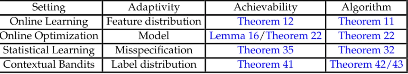
We work in four settings—online learning, online optimization, agnostic statistical learning, and contextual bandits—and for each setting identify an important family of adaptive guarantees for which existing theory and algorithms are unsatisfactory. For each such family we comprehensively characterize the fundamental limits on the degree to which this new type of adaptivity can be achieved, and then design efficient algorithms to achieve this limit. The central contributions are:

• We give tools that permit the systematic development of low-memory adaptive algorithms. We show that whenever a given adaptive rate can be expressed in terms of certain “sufficient statistics” of the data sequence, there exists an online learning algorithm that is only required to keep these sufficient statistics in memory.

• We introduce optimal and efficient algorithms that adapt to problem structure in online convex optimization via online parameter tuning, and characterize limits for this type of adaptivity via connections to the theory of model selection in statistical learning.

• We develop robust statistical learning algorithms that adapt to the degree of model misspecification. Specifically, for logistic regression we design a new improper learning algorithm (via online learning techniques) that attains a doubly-exponential improvement over sample complexity lower bounds for proper learning in the misspecified setting, thereby resolving a COLT open problem of McMahan and Streeter (2012). We then use this algorithm to resolve open problems regarding adaptive algorithms for bandit multiclass classification (Abernethy and Rakhlin, 2009) and online boosting (Beygelzimer et al.,2015), and characterize the extent to which this improvement extends to general hypothesis classes.

• We give a general theory for adapting to problem structure via margin (“margin theory”) in the contextual bandit setting, and develop efficient algorithms to match the guarantees from this framework. Our margin theory for contextual bandits applies at the same level of generality as the classical margin theory in statistical learning, but applies to much more challenging sequential decision making tasks. • We introduce newsequence optimalalgorithms for online supervised learning that

adapt to the structure of the feature distribution. These algorithms are always guar-anteed to match the best possible performance in the i.i.d. statistical learning setting, yet do so without making any assumptions on the data generating process. We characterize the limits of this type of adaptivity through a new connection between online learning and probability in Banach spaces.

Themes In the classical statistical learning model, work beginning with Vapnik and Chervonenkis(1971), has led to a diverse and extensive collection of adaptive performance guarantees. These guarantees are obtained by simple algorithms, and by and large may be understood as consequences of basic phenomena in empirical process theory (Pollard, 1990). A central theme the reader should keep in mind throughout the thesis is:

When can adaptive guarantees from the classical (i.i.d.) statistical learning setting also be achieved for more challenging (e.g., sequential or interactive) learning settings?

Beyond exploring achievability of different notions of adaptivity in the information-theoretic sense, it is also of central importance to understand how the algorithmic principles change when we move beyond the classical setting. Both issues are addressed throughout this thesis.

A second theme is that all of the algorithms we develop make few or no assumptions on the process by which data is generated. Even though we might imagine that the real world is ripe with niceness and problem structure, we lose little by working in such agnostic learning models precisely because theadaptivealgorithms we develop can exploit problem structure whenever instances do happen to be nice.

1.4

Organization

In the remainder of this chapter (Section 1.5), we give a preview of the general approach to analyzing adaptive learning through the equivalence framework. Then, inChapter 2we develop the minimax analysis of adaptive learning formally, showing how to formulate statistical learning, online learning, contextual bandits, and online and stochastic

optimiza-tion in the adaptive minimax framework. From here on, the main content of the thesis is broken into two parts.

Part II: Equivalence of Prediction, Martingales, and Geometry InPart II, we introduce the technical tools that form the core of the thesis. We work in the online learning model, and the main development is the equivalence of adaptive learning, martingale inequalities, and Burkholder functions illustrated inFigure 1.1.

In Chapter 4 we present the equivalence in its simplest form, focusing on the online supervised learning setting with linear losses. As a running example, we illustrate the method by developing a new adaptive algorithm for online matrix prediction. InChapter 5 we present the equivalence in its general form. We also show—via the Burkholder method— how a certain notion of sufficient statistics for online learning leads to low-memory adaptive algorithms. In Chapter 6 we develop generic tools for proving martingale inequalities that arise from the equivalence. We show how adaptive rates in the supervised learning model induce certain “offset” random processes, and that obtaining small upper bounds on these processes is sufficient to demonstrate achievability. We use this approach to recover a number of existing adaptive guarantees, as well as to derive new guarantees.

Part III: New Guarantees for Adaptive Learning In Part III, with the toolbox from Part IIin hand, we proceed to develop new types of adaptive learning guarantees for four settings: statistical learning, online learning, contextual bandits, and online and stochastic optimization. For each setting we identify a new notion of adaptivity, characterize the fundamental limits on the degree to which this adaptivity is achieved, and design efficient algorithms to achieve this limit. Chapter 8 develops sequence-optimal online learning algorithms that adapt to the feature distribution, Chapter 9 introduces algorithms for

model selection and parameter tuning in online convex optimization,Chapter 10gives new algorithms that adapt to model misspecification in logistic regression and related problems, andChapter 11develops margin theory for contextual bandits.

1.5

Highlight: Achievability and Algorithm Design

We close the introduction by offering a taste of the tools developed inPart II. We focus on a setting that is extremely simple, yet completely free of assumptions—online bit prediction—and show how a result ofCover(1967) completely answers two key questions:

1. What properties of an adaptive rate functionφsuffice to guarantee that the rate is achievable?

2. When such a rateφis achievable, what algorithm achieves it?

The bit prediction setting is a special case of theonline learningsetting that features promi-nently in this thesis. The learning process proceeds innrounds: At each stept, the learner randomly selects a prediction distributionqt, receives an outcomeyt∈ {±1}, then samples

its predictionbyt∼qtand suffers the indicator loss1{ybt6=yt}. In this setting, adaptive rates

φ(y1:n)map the bit sequencey1:n =y1, . . . , ynto a risk bound. A rateφis achieved by the

learner if E " 1 n n X t=1 1{_byt6=yt} #

≤φ(y1:n) for every sequencey1:n,

where the expectation is taken with respect to the learner’s randomness. To formulate the minimax value for this setting, we think of a sequential game between the learner and nature. We imagine that in the worst case, nature is an adversary whose goal is to make the learner’s regret toφas large as possible, so that the goal of a minimax optimal learner

is to minimize regret against this adversary. At each round the contribution to regret is a

min-maxproblem conditioned on the history so far: The learner choosesqtto minimize

regret given the history, then nature picks a maximally bad value forytgiven the learner’s

decision, and finally the predictionbytis sampled fromqt. The process is repeated for alln

rounds, giving rise to the following expression for the minimax value:

V(φ) = min q1 max y1 by1E∼q1 . . . min qn max yn by1E∼q1 " 1 n n X t=1 1{_byt 6=yt} −φ(y1:n) # .

So, for what functionsφdoes there exist a strategy for the learner such that this inequality holds (i.e. V(φ) ≤ 0)? Since the adaptive risk inequality is required to hold for every sequence y1:n, we are free to try some examples to deduce the important properties of

φ. As a particular choice, let1, . . . , nbe a sequence of independentRademacher random

variables, i.e. fair coin flips in{±1}, and chooseyt=t. Since the learner’s strategy at time

tonly depends on1, . . . , t−1, it is easy to see thatE[1{byt 6=yt}] =

1

2 for any learner. Since this holds at each round, we conclude that anecessarycondition for achievability is that

E

[φ(1:n)]≥

1

2. (1.7)

This condition is necessary, but is it sufficient? Suppose thatφis additionallystable, in the sense that

|φ(1, . . . , t, . . . , n)−φ(1, . . . , 0t, . . . , n)| ≤

1 n

for all sequences1:n, all choices for0t, and all timest. Cover’s result is that in this case,

the answer isyes.

Lemma 1(Cover(1967)). Letφbe any stable adaptive rate function. Thenφis achievable if and only if E[φ(1:n)]≥ 1₂. Furthermore, any rateφsatisfying this condition is achieved

by the algorithm that choosesqtto be the unique distribution over{±1}with mean

µt =n· E t+1:n

Cover’s result is proved through a potential function argument, which is a recurring theme in this thesis. The characterization has two favorable properties:

1. The condition for achievability isalgorithm-independent. Checking for existence of a prediction strategy that achievesφis as simple as checking the probabilistic inequality E[φ(1:n)]≥ 1₂.

2. It admits an explicit algorithm. That is, once a rateφis known to be achievable, we can efficiently compute the strategy that obtainsφand use it to make predictions.1

Cover’s characterization is quite elegant and will serve as an inspiration for our results going forward, but it has a number of insufficiencies that must be addressed if we wish to apply the framework to solve real-world learning challenges. To note a few:

• The learning problem to which the characterization applies does not have covariates or contexts. This prevents it from being applied to basic classification and regression tasks.

• The learner’s decision space{±1}is quite simple; to develop adaptive algorithms for, e.g. optimization, we should accomodate rich output spaces, such as subsets of Rdor even infinite-dimensional Banach spaces.

• The characterization only applies to the classification loss. To accommodate standard problems in learning and statistics, we would like to handle other losses, such as the square loss, logistic loss, and so forth. Characterizing the correct statistical complexity and developing optimal algorithms for general losses is far from trivial, even in the case of uniform (non-adaptive) rates.

1_{It is straightforward to show via concentration that the expectation in the strategy’s definition can be}

approximated arbitrarily well with polynomially many samples. This strategy achievesφup to an arbitrarily small additive constant.

• In the supervised learning problems, adaptive rates typically incorporate regret against a benchmark class of modelsF. For example, we might have

φ(x1:n, y1:n) = inf f∈F 1 n n X t=1 `(f(xt), yt) +B(x1:n, y1:n),

where B is another function that we refer to as an adaptive bound on the regret to F. What properties of F influence achievability? Are the requirements on φ more stringent whenF is a class of neural networks than when it is a class of linear functions? In the case of uniform rates (Bis constant), this question is addressed in a line of work beginning withRakhlin et al.(2010); we extend this to handle adaptivity. • The result is specialized to “full information”, wherein the learner completely ob-serves the feedback chosen by nature. Can we obtain similar characterizations for the complexity of adaptive learning when the feedback is only partially observed? This is the essential difficulty of contextual bandits.

These questions are far from trivial, and the main results in this thesis may be understood as answering them with varying levels of completeness.

Proof ofLemma 1. We must prove that E[φ(1:n)] ≥ 1₂ and stability are sufficient for

achievability, and that the strategyqtachievesφunder these conditions.

LetUt(y1, . . . , yt) = n₂−_nt −Et+1:nφ(y1, . . . , yt, t+1, . . . , n). Then clearly it holds that 1 n n X t=1 1{y_bt6=yt} −φ(y1, . . . , yn)≤ 1 n n X t=1 1{y_bt6=yt}+Un(y1, . . . , yn).

To prove the result, it suffices to show inductively that for each 1 ≤ t ≤ n, playing the prescribed strategy ensures

E b yt∼qt 1 n1{byt 6=yt}+Ut(y1, . . . , yt) ≤Ut−1(y1, . . . , yt−1),

for any outcomeyt. This implies that the strategy guarantees E " 1 n n X t=1 1{y_bt6=yt} −φ(y1, . . . , yn) # ≤U0(·),

and we haveU0(·) = 1₂ −Eφ(1, . . . , n)≤0under the assumption thatE[φ(1:n)]≥ 1₂.

We proceed with the inductive proof. Since qt is a distribution over {±1}, it can

be parameterized by its mean µt ∈ [−1,+1]. With this parameterization, we have

Ebyt∼qt

₁

n1{byt 6=yt}

= (1−µtyt)

2n . Consequently, the minimax value at time t can be

writ-ten min µt max yt∈{±1} (1−µtyt) 2n +Ut(y1, . . . , yt)

We chooseµtso that the value inside the brackets is constant regardless of the outcomeyt,

i.e. to guarantee

(1−µt)

2n +Ut(y1, . . . , yt−1,+1) =

(1 +µt)

2n +Ut(y1, . . . , yt−1,−1),

which results in the strategy µt = n · (Ut(y1, . . . , yt−1,+1)−Ut(y1, . . . , yt−1,−1)). The stability property implies that this choice satisfiesµt∈[−1,+1], and by direct calculation

it is seen that we indeed have

max yt∈{±1} (1−µtyt) 2n +Ut(y1, . . . , yt) =Ut−1(y1, . . . , yt−1).

For further results regarding Cover’s characterization we refer the reader toRakhlin and Sridharan(2016b).

1.6

Bibliographic Notes

From Part III,Chapter 8 is also based on Foster et al. (2017b). Chapter 9 is based on a joint work with Satyen Kale, Mehryar Mohri, and Karthik Sridharan (Foster et al.,2017a). Chapter 10 is based on a joint work with Satyen Kale, Haipeng Luo, Mehryar Mohri, and Karthik Sridharan (Foster et al.,2017a).Chapter 11is based on a joint work Akshay Krishnamurthy (Foster and Krishnamurthy,2018).

1.7

Notation

General Notation 1{E}will denote the indicator for a meaurable eventE, andP{E}will denote the probability of the event when the measure is clear from context.Ewill denote expectation. WhenP is a probability distribution andXis a formal variable, the notation “X ∼P” will be interpreted to mean “X is distributed according toP.”

The notationσ(X)will denote the Borelσ-algebra for a random variableX.

We define sgn(x) =            1, x >0. 0, x= 0. −1, x <0.

For an integerk ∈_Nwe define[k] ={1, . . . , k}. For scalarsa, b∈_Rwe adopt the notation a∨b = max{a, b}anda∧b= min{a, b}.

We usea:=bto mean “ais defined to be equal tob” and likewise usea =:bto mean “bis defined to be equal toa.”

∆dwill denote the simplex inddimensions. More generally, we use∆Aor∆(A)to denote

Asymptotic Notation For functions f, g : _Rd _→

R, we say f ∈ O(g) if there exists a constantC such for allRd-valued sequences(αn)n≥1withlimn→∞αni → ∞for alli,

lim sup

n→∞

f(αn₎

g(αn₎ ≤C.

Likewise, we sayf ∈Ω(g)if for all such sequences,

lim inf

n→∞

f(αn) g(αn₎ ≥C.

We sayf ∈O˜(g)andf ∈Ω(˜ g)iff ∈O(g·polylog(g))andf ∈Ω(g/polylog(g))respectively.

Analysis Throughout this thesisk·kwill denote a norm andk·k_? will denote the dual. Specific norms include the`p norms, denotedk·k_p, the Schattenp-norms, denotedk·k_Sp,

the spectral normk·k_σ, and the nuclear normk·k_Σ. Bd

p will denote thed-dimension unit`p

ball.

We will use the notation(B,k·k)to denote a Banach spaceBequipped with normk·k, and will let(B?_,k·k

?)denote the dual space. Whenx∈Bandy∈B?,hy, xidenotes the dual

pairing, which coincides with the inner product whenBis a Hilbert space.

Let Sd denote the set of symmetric matrices in Rd×d, Sd+ denote the set of positive-semidefinite (psd) matrices, and Sd++ denote the set of positive-definite matrices. For compatible matricesAandB,hA, Bi=tr(AB>)is the standard matrix inner product.

A twice-differentiable functionf :B→_Ris said to beβ-smooth with respect tok·kif its gradient satisfiesk∇f(x)− ∇f(y)k_? ≤βkx−yk. We will use the phrase “smooth norm” to refer to any norm for which the functionΨ(x) = 1₂kxk2 isβ-smooth with respect tok·k. This is equivalent to the statement that the following inequality holds for all x, y ∈ B:

A Banach space(B,k·k)is said to be(2, D)-smooth if for allx, y ∈B(Pinelis,1994), kx+yk2+kx−yk2 ≤2kxk2+ 2D2kyk2.

From this definition it is seen that any Banach spaces with a β-smooth norm has the

(2,pβ/2)-smoothness property.

A space (B,k·k) is said to have martingale type 2 with constant β if there exists some

Ψ :B→_Rsuch that 1₂kxk2 ≤Ψ(x),Ψisβ-smooth with respect tok·k, andΨ(0) = 0(Pisier, 1975).

For a function f : X → _R, we let f? denote the Fenchel dual, i.e. f?(y) = sup_x∈X[hy, xi −f(x)].

Martingales Let(Xt)t≥1 be a sequence of real- orB-valued random variables adapted to a filtration(Ft)_t≥0. The sequence is said to bemartingaleif

E[Xt | Ft−1] =Xt−1 ∀t, and is said to be amartingale difference sequence(MDS) if

E[Xt| Ft−1] = 0 ∀t.

Let(t)_t≥1 be a sequence of Rademacher random variables. Adyadicmartingale difference sequence is a MDS adapted to the filtrationFt = σ(1, . . . , t). Any dyadic MDS can be

written as

Xt =t·xt(1, . . . , t−1), wherext(1, . . . , t−1)is apredictable process.

Miscellaneous Learning Notation We will frequently use the notationx1:n =x1, . . . , xn

xt[i]to denote thetth vector’sith coordinate. We make reference to the following standard

loss functions.

• Indicator loss/zero-one loss:`(<sub>b</sub>y, y) =1{<sub>b</sub>y6=y}. • Absolute loss:`(_by, y) =|y_b−y|.

• Square loss:`(y, y<sub>b</sub> ) = (y<sub>b</sub>−y)2. • Logistic loss:`(y, y_b ) = log 1 +e−yyb

CHAPTER 2

LEARNING MODELS AND ADAPTIVE MINIMAX FRAMEWORK

A central aim of this thesis is to give a unified formalism for analyzing adaptive learning guarantees in real-world settings. This section lays the groundwork for this approach by developing the adaptive minimax analysis framework outlined in the introduction formally. We instantiate the general framework for learning settings that feature throughout the thesis: statistical learning, online learning, online optimization, and contextual bandits.

2.1

Adaptive Minimax Value

We work in the language of statistical decision theory (Van der Vaart,2000;Lehmann and Casella,2006). The class of possible instances in nature is described by a set distributions P ={Pθ |θ∈Θ}over a domainS, parameterized by some setΘ(e.g., for mean estimation,

P could be a set of gaussian distributions withΘdescribing the set of means). Nature selects an elementθ ∈Θ, and the learner receives a sampleS ∼Pθ. LettingΘb denote the

set ofdecisions, the learner outputs a (potentially randomized) decision functionθb:S →Θb.

For a fixedlossorriskfunctionalL:Θb ×Θ→R, the learner’s expected risk is measured

via E Pθ h L(θb(S), θ) i . (2.1)

As in the introduction, we let an adaptive rate functional φ : S ×Θ → _Rbe given, and evaluate the learner’s risk relative toφ, i.e.

E Pθ h L(θb(S), θ)−φ(S, θ) i .

If this quantity is bounded by zero, the functionalφ (or “rate”, for short) is said to be achievedby the ruleθb. Note that the rateφcaptures both niceness in the instanceP_θand

niceness of the outcomeSitself.

The risk relative to the rateφimmediately lends itself to minimax analysis, thereby extend-ing Wald’s minimax principle (Wald,1939) to incorporate adaptivity. This is formalized by theminimax achievabilityforφ, defined via

V(φ) = inf b θ sup θ∈ΘPEθ h L(bθ(S), θ)−φ(S, θ) i . (2.2)

All learning models studied in this thesis share the following structure, which is a special case of the general decision setup(2.1): The observationS will be a sequence of examples of the formz1, . . . , znwith eachztbelonging to some setZ. Individual examples may be

drawn i.i.d. (statistical learning) or selected interactively based on the learner’s decisions (online learning). The learner makes decisions ybbelonging to a set D, and the loss for

a given prediction-example pair will be`(<sub>b</sub>y, z), where ` : D × Z → _R. The final metric through which performance is measured is the value of the function`(either empirical or expected, depending on the setting) relative to an adaptive rateφ.

Warmup: PAC Learning and Statistical Estimation We first consider a setting that en-compasses classical PAC learning (Valiant,1984), as well as the basic statistical task of statistical estimation with a well-specified model (e.g. Tsybakov(2008)). We takeSto be a collection of examples{(xt, yt)}n_t=1inX × Y =:Z drawn i.i.d. from a joint distribution

PX×Y (so thatzt= (xt, yt)). The marginal distributionPX is arbitrary and the conditional

distributionPY|X is defined via

Y =f?(X) +ξ, (2.3)

wheref?belongs to amodel classF ⊆(X → Y)andE[ξ|X] = 0. The classF serves as a model for nature. A learning rule takes as input the sample setS and returns a predictor y : X →Y (so thatD = (X → Y)). We define a point-wise loss` : Y × Y →R, and the

risk of a particular predictorbyis given by`(y, zb ) = `(yb(x), y). The final notion of risk in (2.1)is E S h E P `(ybS(x), y) i .

Taking Yb = Y = {±1}, `(y, y_b ) = 1{y_b6=y} and ξ = 0 recovers PAC learning, while

settingY =_Rand`(<sub>b</sub>y, y) = (<sub>b</sub>y−y)2 or`(y, y_b ) = |y_b−y|recovers classical nonparametric regression.

The minimax risk is

V_npac(F) = inf b y sup_{PX P}sup Y|X realizable E S h E P `(ybS(x), y) i ,

while the minimax achievability for a rateφis Vpac n (φ) = inf b y sup_{PX P}sup Y|X realizable E S h E P `(byS(x), y)−φ(x1:n, y1:n, PX, PY|X) i . (2.4)

We see that the adaptive rateφcan depend on the particular draw of examples{(xt, yt)}n_t=1,

as well as the true functionf?_{and marginal distributionP}

X. Nice instances for this setting

may include functionsf?_{for which the decision boundary is simple—at least simple in}

areas where the marginal distributionPX is concentrated (Boucheron et al.,2005)—-or

might include instances where the variance ofξis low.

2.2

Statistical Learning

Existence of a functionf? that realizes the modelPY|X is a rather strong assumption. We

would like to develop methods that enjoy prediction guarantees when this assumption is violated, but hopefully can adapt when the assumptiondoeshold.

For classification, theagnostic PAC framework(Haussler,1992;Kearns et al.,1994) generalizes PAC learning to the case where the joint distribution PX×Y is arbitrary. For regression,

Protocol 1Statistical Learning Nature selects distrbutionPX×Y.

Learner receives samplesS = (x1, y1), . . . ,(xn, yn)i.i.d. fromPX×Y.

Learner returns predictory_bS ∈(X →Yb). (For proper learning, b

yS ∈ F.)

this is referred to as themisspecified modelsetting in nonparametric statistics (Nemirovski, 2000;Tsybakov,2008) and aggregation (Tsybakov,2003;Lecu´e and Rigollet,2014). The distribution PX×Y may be completely unrelated to the model class F, and there may

indeed be distributionsP for which the expected riskE`(f(x), y)is large for allf ∈ F (for classification, consider the case where labels are drawn uniformly at random). Clasically, instead of looking at minimax risk in the sense of`, agnostic learning considersminimax regret:1 Viid n (F) = inf b y _Psup_X×Y ES E`(byS(x), y)−<sub>f</sub>inf<sub>∈F</sub>E`(f(x), y) . (2.5)

Here the word “regret” reflects that performance is measured relative the classF, which serves as abenchmarkorcomparator. A bound on the right-hand-side of this expression is also referred to as anexact oracle inequalityin statistics (Tsybakov,2003;Lecu´e and Rigollet, 2014).

In this case, a natural way to define minimax achievability for an adaptive rateBis

V_niid(F,B) = inf b y _Psup X×Y E S E`(ybS(x), y)− inf f∈FE`(f(x), y)− B(x1:n, y1:n, PX×Y) . (2.6)

Note on Terminology. Throughout this thesis we use the symbolφfor adaptive rates that bound risk and the symbolBfor adaptive rates that bound regret.

This formulation already subsumes many notions of adaptivity proposed in statistical learning theory (Boucheron et al.,2005). To capture further notions of adaptivity, such as PAC-Bayesian bounds (McAllester,1999), we can allow the adaptive rateBto depend on 1_{Note that minimax regret still falls into the statistical decision theory framework for the right choice ofL.}

the benchmark itself, i.e. V_niid(F,B) = inf b y _Psup X×Y E Ssup_f∈F[E`(byS(x), y)−E`(f(x), y)− B(f ;x1:n, y1:n, PX×Y)]. (2.7)

Of course, we can go further and return to adaptive ratesφthat upper bound the expected risk itself, with the understanding that any achievable rate of this form must be large for some instancesPX×Y: V_niid(φ) = inf b y _Psup X×Y E S[E`(ybS(x), y)−φ(x1:n, y1:n, PX×Y)]. (2.8)

This formulation is syntactically very close to that ofVpac

n (φ)in(2.4), but the key difference

is that we have dropped the assumption on the conditional distribution.

2.3

Online Supervised Learning

While the agnostic statistical learning setting is certainly more general than the PAC framework, it still makes a strong assumption, namely that the examples{(xt, yt)}n_t=1 are

i.i.d. An alternative isonline learning, where data examples arrive one-by-one and the learner must make predictions on demand, and the data generating process is arbitrary or

Protocol 2Online Supervised Learning

1: fort= 1, . . . , ndo

2: Nature providesxt∈ X.

3: Learner selects randomized strategyqt∈∆(Yb).

4: Nature provides outcomeyt∈ Y.

5: Learner drawsbyt ∼qtand incurs loss`(ybt, yt).

6: end for

even adversarial.

The exact setup is as follows. The learner plays n rounds, and for each round t they receive an instancext and must produce a predictionybtusing the new instance as well

as the previous observations (x1, y1,). . . ,(xt−1, yt−1). Nature chooses the true outcome yt, and the cumulative loss is given by _n1Pn_t=1`(ybt, yt). As in agnostic learning, classical

(non-adaptive) online learning evaluates learning procedures based on theirregretagainst a benchmark classF: 1 n n X t=1 `(<sub>b</sub>yt, yt)− inf f∈F 1 n n X t=1 `(f(xt), yt).

Like the bit prediction setting in the introduction, we formulate minimax analysis for online learning by imagining a game between the learner and nature. At each round the contribution to regret is amax-min-maxproblem conditioned on the history so far: Nature choosesxtto maximize regret, then the learner choosesybtto minimize regret given nature’s

decision. Finally, nature picks a maximally bad value forytbased on the learner’s decision.

The process is repeated for all nrounds, giving rise to the following expression for the minimax value: V_nol(F) = sup x1 inf b y1 sup y1 . . .sup xn inf b yn sup yn " 1 n n X t=1 `(y<sub>b</sub>t, yt)− inf f∈F 1 n n X t=1 `(f(xt), yt) # .2

We adopt the following notation to write expressions of this type more succinctly: Vol n(F) = ⟪sup xt inf b yt sup yt ⟫ n t=1 " 1 n n X t=1 `(y<sub>b</sub>t, yt)− inf f∈F 1 n n X t=1 `(f(xt), yt) # , (2.9)

where the notation ⟪?⟫n_t=1 denotes interleaved application of the operator ? from time t = 1, . . . , n. The difference of the cumulative losses of the forecaster and the loss of any particular benchmark f ∈ F, which we refer to to as regret against f, is denoted

Reg_n(f) =Pn

t=1`(byt, yt)−`(f(xt), yt).

Turning to adaptivity, we can either ask for an adaptive regret bound Band look at the minimax achievability ofBvia

Vol n(F,B) = ⟪sup xt inf b yt sup yt ⟫ n t=1 sup f∈F " 1 n n X t=1 `(y<sub>b</sub>t, yt)− 1 n n X t=1 `(f(xt), yt)− B(f;x1:n, y1:n) # , (2.10) 2_{Online supervised learning fits into the decision theory framework by taking}

b

or we can ask for a general adaptive risk boundφand look at minimax achievability via Vol n(φ) = ⟪sup xt inf b yt sup yt ⟫ n t=1 " 1 n n X t=1 `(y_bt, yt)−φ(x1:n, y1:n) # . (2.11)

From this definition, we see that for anyφthere always exists an algorithm that guarantees

1 n n X t=1 `(y_bt, yt)≤φ(x1:n, y1:n) +V(φ) ∀sequencesx1:n,y1:n.

In a slightly more general setting,Protocol 2, we allow the learner to be randomized, i.e. to select a distributionqtfrom which the predictionbytis sampled onlyafteryt.

3 _{For such}

randomized learners, minimax achievability is written Vol n(φ) =⟪sup xt inf qt sup yt E b yt∼qt ⟫ n t=1 " 1 n n X t=1 `(y_bt, yt)−φ(x1:n, y1:n) # . (2.12)

The online-to-batch principle, dating back to the very genesis of learning theory (Vapnik and Chervonenkis,1968), implies that for any rateφ(x1:n, y1:n),

Vpac n (φ)≤ V iid n (φ)≤ V ol n(φ). (2.13)

An important development in this thesis is that while there are indeed ratesφfor which Vol

n(φ) Vniid(φ), for many types of adaptivity of practical interest we have Vnol(φ) ≤

c· Viid

n (φ)for some small constantc, meaning that even when offline learning is the end

goal we pay essentially no price for considering the more general framework, and can therefore leverage the advantages (e.g. single pass learning) that it provides.

2.4

Online Convex Optimization

Online convex optimization (OCO) is close relative of the online supervised learning setting, in which a learner makes vector-valued predictions and is evaluated against

an adversarially chosen sequence of convex loss functions. This model is useful for solving large-scale empirical risk minimization problems for machine learning, as well as for directly performing minimization of the population risk in statistical learning and stochastic optimization. In particular, regret bounds in the online convex optimization immediately imply upper bounds on theoracle complexityof stochastic convex optimization.

We describe a randomized variant of the OCO setting here. We playnroundst= 1, . . . , n. At each round the learner chooses a distributionqtover a convex setW. Nature chooses a

convex lossft, and the learner sampleswt∼qtand experiences lossft(wt). Depending on

the application nature may be constrained to choose, for example,1-Lipschitz or1-smooth convex functions. We letZ denote their set of decisions.

Protocol 3Online Convex Optimization

fort = 1, . . . , ndo

Learner selects strategyqt∈∆(W)for convex decision setW.

Nature selects convex lossft: W →R.

Learner drawswt∼qtand incurs lossft(wt). end for

In online convex optimization the usual notion of performance is regret relative to the benchmark constraint setW. In particular, the (non-adaptive) minimax value is given by

Voco n (W) = ⟪ inf qt∈∆(W)_fsup_t∈ZwtE∼qt ⟫ n t=1 " 1 n n X t=1 ft(wt)− inf w∈W 1 n n X t=1 ft(w) # . (2.14)

To analyze adaptive regret boundsB, minimax achievability is defined through Voco n (W,B) = ⟪ inf qt∈∆(W)_fsup_t∈ZwtE∼qt ⟫ n t=1 sup w∈W " 1 n n X t=1 ft(wt)− 1 n n X t=1 ft(w)− B(w;f1:n) # , (2.15) and for adaptive risk bounds minimax achievability is given by

V_noco(φ) =⟪ inf qt∈∆(W)_fsupt∈Zwt∼Eqt ⟫ n t=1 " 1 n n X t=1 ft(wt)−φ(f1:n) # . (2.16)

Online convex optimization can be thought of as a special case of the online supervised

literature by a focus on appropriately handling the complexity of the output space, which is typically high-dimensional in OCO applications.

2.5

Contextual Bandits

Online supervised learning and online convex optimization are very general and powerful models that are useful both for streaming learning settings and (via online-to-batch) offline statistical learning. One drawback is that both settings make the assumption that the entire lossfunction`(·, zt)is observable, while in many applications we may only observe the

value`(y_bt, zt) under the learner’s decision. Such a model is appropriate in news article

recommendation and related sequential decision making problems: The learner repeatedly suggests news articles to users on a website and would like to improve their performance over time, but they only observe whether each user views the article that was suggested, not which of the potential articles the user would have preferred in hindsight (Li et al., 2010). Thecontextual banditmodel formalizes this problem.

Protocol 4Contextual Bandit

fort = 1, . . . , ndo

Nature provides contextxt∈ X.

Learner selects randomized strategyqt ∈∆(A).

Nature provides outcome`t�