Cost-sensitive feature selection for Support Vector
Machines
S. Ben´ıtez-Pe˜naa,b,∗, R. Blanqueroa,b, E. Carrizosaa,b, P. Ramirez-Coboa,c
aIMUS. Universidad de Sevilla. 41012 Sevilla. Spain
bDepartamento de Estad´ıstica e Investigaci´on Operativa. Universidad de Sevilla. 41012
Sevilla. Spain
cDepartamento de Estad´ıstica e Investigaci´on Operativa. Universidad de C´adiz. 11510
Puerto Real, C´adiz. Spain
Abstract
Feature Selection (FS) is a crucial procedure in Data Science tasks such as Classification, since it identifies the relevant variables, making thus the classifi-cation procedures more interpretable and more effective by reducing noise and data overfit. The relevance of features in a classification procedure is linked to the fact that misclassifications costs are frequently asymmetric, since false positive and false negative cases may have very different consequences. How-ever, off-the-shelf FS procedures seldom take into account such cost-sensitivity of errors.
In this paper we propose a mathematical-optimization-based FS procedure embedded in one of the most popular classification procedures, namely, Support Vector Machines (SVM), accommodating asymmetric misclassification costs. The key idea is to replace the traditional margin maximization by minimizing the number of features selected, but imposing upper bounds on the false positive and negative rates. The problem is written as an integer linear problem plus a quadratic convex problem for SVM with both linear and radial kernels.
The reported numerical experience demonstrates the usefulness of the pro-posed FS procedure. Indeed, our results on benchmark data sets show that a
∗Corresponding author
Email addresses: [email protected](S. Ben´ıtez-Pe˜na),[email protected](R. Blanquero),[email protected](E. Carrizosa),[email protected](P. Ramirez-Cobo)
substantial decrease of the number of features is obtained, whilst the desired trade-off between false positive and false negative rates is achieved.
Keywords: Classification, Data Science, Support Vector Machines, Feature Selection, Integer Programming, Sparsity
1. Introduction
Supervised Classification is one of the most important tasks in Data Science, e.g. [1, 2], full of challenges from a Mathematical Optimization perspective, e.g. [3, 4, 5, 6, 7, 8, 9, 10, 11, 12, 13, 14, 15, 16, 17].
In its most basic version, we are given a setIof individuals, each represented
5
by a vector (xi, yi), where xi ∈ RN is the so-called feature vector, and yi ∈
C ={−1,1} is the membership of individual i. A classifier Ψ, i.e., a function Ψ : RN −→ C, is sought to assign labels c ∈ C to incoming individuals for which the feature vectorxis known but the labely is unknown and estimated through Ψ(x).
10
The different classification procedures differ in the way the classifier Ψ is obtained from the data set I. A frequent approach consists of reducing the search of the classifier to the resolution of an optimization problem, see [9]. This is the case, among many others, of the state-of-the-art classifier known as Support Vector Machines (SVM), [9, 18, 19, 20], addressed in this paper.
15
In SVMwith linear kernel, Ψ takes the form
Ψ(x) = 1, ifw>x+β≥0 −1, else, (1)
wherew∈RN andβ∈Rare obtained as the optimal solution of the following
convex quadratic programming formulation with linear constraints minw,β,ξ w>w+CPi∈Iξi
s.t. yi(w>xi+β)≥1−ξi, i∈I
ξi≥0 i∈I.
HereC >0 is theregularization parameter, which needs to be tuned, andξi≥0 is a penalty associated to misclassifying individual i in the so-called training
20
sampleI.
An apparently innocent extension of (1) is given by
Ψ(x) = 1, ifw>φ(x) +β ≥0 −1, else, (3)
whereφ:RN → Hmaps the originalN features into a vector space of higher di-mension, andwandβare obtained by solving an optimization problem formally identical to (2), but taking place in the spaceHinstead ofRN
25
minw,β,ξ w>w+CPi∈Iξi
s.t. yi(w>φ(xi) +β)≥1−ξi, i∈I
ξi ≥0 i∈I.
(4)
In this case, the classifier is usually obtained by solving, instead of (4), its dual,
maxα P i∈Iαi− 1 2 P i,j∈IαiyiαjyjK(xi, xj) s.t. P i∈Iαiyi = 0 0≤αi≤ C2, i∈I, (5)
where K(x, x0) = φ(x)>φ(x0) is the so-called kernel function. From the op-timal solution to (5) and taking into account the complementarity slackness conditions,w andβ in (3) are obtained. In particular,
30 w>w = X i,j∈I αiyiαjyjK(xi, xj), (6) w>φ(x) = X i∈I αiyiK(xi, x). (7)
See e.g. [9, 18, 19, 20] for details.
The classifier uses all the features involved in the problem, both in (1) and (3), which may be rather problematic if the dimensionNof the data set is large, since it will be hard to identify which features are significant for classification purposes. It is then advisable to perform Feature Selection (FS), [21, 22, 23,
24, 25, 26, 27, 28, 29, 30], in order to reduce the set of features and obtain an appropriate trade-off between classification accuracy and sparsity.
A mountain of different FS procedures are found in the literature, some inde-pendent of the classification procedure (FS is performed in advance, based e.g. on the correlation between each feature and the label) and others embedded in
40
the classification procedure. The latter is the approach considered in this paper, since we aim to obtain an SVM-based classifier, and, at the same time, perform the selection of the features. The core idea is the optimization problem to be solved: instead of maximizing the margin, as in the traditional SVM, we seek the classifier with lowest number of features, but without damaging too much
45
the original performance. In order to be able to control the classifier’s perfor-mance, we will make use of constraints as in [31]. Specifically, the formulation of the constrained SVM with linear kernel is
minw,β,ξ w>w+CPi∈Iξi s.t. yi(w>xi+β)≥1−ξi, i∈I 0≤ξi≤L(1−ζi) i∈I µ(ζ)`≥λ` `∈L ζi∈ {0,1} i∈I. (8)
In essence, this is simply the formulation for the SVM with linear kernel, to which performance constraints (µ(ζ)` ≥ λ`) have been added, see [31] for the
50
details. Its (partial) dual formulation is minα,β,ξ,ζ P i,j∈I αiyiαjyjK(xi, xj) +CPi∈Iξi s.t. yi(P j∈I αjyjK(xj, xi) +β)≥1−ξi, i∈I P i∈I αiyi= 0 0≤αi≤C/2 i∈I 0≤ξi≤L(1−ζi) i∈I µ(ζ)`≥λ` `∈L ζi∈ {0,1} i∈I. (9)
with general kernel and constraints in the performance measures, as in (8). For more information about how formulation (9) is obtained, the reader is referred to the Appendix. Note that, while mathematical optimization problems addressed
55
in the statistical literature are, traditionally, as (2) or (5), nonlinear programs in continuous variables, our approach involves integer variables, which define harder optimization problems. However, Integer Programming has shown to be rather competitive thanks to the impressive advances in (nonlinear) integer programming, as demonstrated in recent papers addressing different topics in
60
data analysis, [32, 33, 24, 7, 8, 34].
The remainder of the paper is structured as follows. In Section 2 we present the new FS methodology for SVM, by proposing mathematical optimization programs. For either linear or nonlinear kernels, we reduce the problem to solving a standard linear integer program plus, eventually, a quadratic convex
65
problem. Our FS approach is empirically tested. In Section 3 we describe how the different experiments have been carried out. Then, the results of those ex-periments are shown in Section 4. Comparisons between the use of linear and radial kernels, and between the standard linear SVM with and without embed-ded FS are proviembed-ded. The paper ends with conclusions and possible extensions
70
in Section 5.
2. Cost-sensitive Feature Selection
In this section we present a novel linear formulation for SVM where classi-fication costs are modeled via certain constraints, and where, in addition, a FS approach is embedded in such a way that only the relevant features are
consid-75
ered. In Section 2.2 the FS approach using a linear or an arbitrary kernel is addressed.
In order to cope with classification costs, first we recall some performance measures, namely,
• TPR (True Positive Rate): P(w>X+β >0|Y = +1)
80
• Acc (Accuracy): P(Y(w>X+β)>0).
The objective is to classify using a reduced set of features in such a way that certain constraints over the performance, such as T P R ≥λ1 or T N R ≥λ−1 (for threshold valuesλ1,λ−1∈[0,1]), are fulfilled.
85
Note that the pair (X, Y) is a random vector (with unknown distribution) from which a sample {(xi, yi)}i∈I is generated. This implies that T P R and
T N Rare statistics and therefore, they should be estimated from sample data. This leads to the empirical constraintsT P R[ ≥λ∗1andT N R\≥λ∗−1, forλ∗1≥λ1 andλ∗
−1≥λ−1, where the performance measures are replaced by their sample
90
estimates. Two possible choices, which shall be explored in this work, are
λ∗1 = λ1 and
λ∗
−1 = λ−1,
(10)
or the more conservative approach based on Hoeffding inequality,
λ∗1 = λ1+ r−logα 2|I+| and λ∗−1 = λ−1+ r −logα 2|I−| , (11)
whereαis the significance level for the hypothesis test whose null hypothesis is eitherT P R≤λ1or T N R≤λ−1. See [31] for more details.
Note that it is straightforward to extend our results to the case in which
95
measurement costs are associated with the features, as in e.g. [35], and then the minimum-cost feature set is sought instead.
2.1. The cost-sensitive FS procedure
Assume that we have a linear kernel, i.e., K(x, x0) = x>x0, and thus the SVM with all features is obtained by solving (2). We state the feature
selec-100
tion problem as a Mixed Integer Linear Program. Consider an auxiliary vari-ableζi that takes the value 1 if record i is correctly classified and is equal to 0 otherwise. Hence, estimates of TPR and TNR from sample I are given by
[
T P R=P
i∈Iζi(1+yi)/Pi∈I(1 +yi) andT N R\=Pi∈Iζi(1−yi)/Pi∈I(1−yi), respectively. Associated with each featurek, 1≤k≤N, we define the variable
105
zk taking the value 1 if feature k is selected for classifying, and 0 otherwise. Hence, the optimization problem that defines a linear classifier (hyperplane) taking into account the classification rates and in which a FS procedure is inte-grated is given by minw,β,z,ζ N P k=1 zk s.t. yi(w>xi+β)≥1−L(1−ζi), ∀i∈I P i∈Iζi(1−yi)≥λ∗−1 P i∈I(1−yi) P i∈Iζi(1 +yi)≥λ∗1 P i∈I(1 +yi) |wk| ≤M zk ∀k∈1, . . . , N ζi∈ {0,1} ∀i∈I zk ∈ {0,1} ∀k∈1, . . . , N (P1)
whereM andLare sufficiently large numbers.
110
Let us discuss the rationality of the formulation (P1). The number of fea-tures used for classifying is to be minimized in the objective. The first constraint identifies which individuals are correctly classified, since, as soon asζi= 1,the score Ψ(xi) is forced to be Ψ(xi) ≥1 (ifyi = 1) or Ψ(xi)≤ −1 (ifyi =−1). Furthermore, the constantP
i∈I(1−yi) is equal to two times the cardinality of
115
the set{i∈I:yi=−1}, whereasPi∈Iζi(1−yi) yields two times the number of individuals correctly classified in the class−1. Hence, the second and third constraints force respectively the fraction of individuals with labelyi=−1 (re-spectively,yi = 1) correctly classified to be at leastλ∗−1 (respectively, at least
λ∗1). Finally, the fourth constraint forces to select those featureskwithzk = 1.
120
Note that an SVM classifier has not been built yet, since the margin has not been maximized. The next section shall address such problem by using the SVM either with the linear kernel or with an arbitrary one.
2.2. Cost-sensitive sparse SVMs: linear vs arbitrary kernels
of the classifier with linear kernel. Hence, the sparse SVM that controls the classification rates is formulated as
minω,β,ξ,z N P j=1 w2 jzj+CPi∈Iξi s.t. yi(P N j=1ωjzjxij+β)≥1−ξi, ∀i∈I 0≤ξi≤M(1−ζi) ∀i∈I ζi ∈ {0,1} ∀i∈I P i∈Iζi(1−yi)≥λ∗−1 P i∈I(1−yi) P i∈Iζi(1 +yi)≥λ ∗ 1 P i∈I(1 +yi) (P2)
Note that (P2) is defined similarly as a standard linear SVM optimization
125
problem. The slight difference is that in (P2) only the variables selected by the FS approach described in Section 2.1. are considered. This means that the values ofz in (P2) are those obtained in problem (P1). Note too that the constraints concerning the performance measures are also added here.
Now, assume the SVM classifier has the form (3), and an arbitrary kernel functionK(x, x0) =φ(x)>φ(x0) is used instead of the linear one. See e.g. [9, 18, 19, 20] for details. Although formally similar, the case of an arbitrary kernel
Kimplies that, if an FS procedure as (P1) is desired, nonlinear constraints are involved and thus the optimization problem is harder to solve. For this reason, instead of coping with such hard problem, we propose an alternative strategy: first, (P1) is solved (as before), and then the SVM classifier (with the selected kernel) is built, using only the features selected in the problem described in Section 2.1. In what follows we focus on the radial kernel, even though one can consider any arbitrary kernel K. First, we define the binary variables z
identifying the features which are selected for classifying. The choice of the features, identified with the vectorz, leads to the kernelKz,defined as
Kz(x, x0) =exp −γ N X k=1 zk(x(k)−x0(k))2 !! ,
wherex(k)denotes thek-th component of vectorx.
Forz (and thusKz) fixed, the aim is to solve (4), but replacing the terms w>w and w>φ(xi), respectively, by the expressions (6) and (7), apart from adding the constraints related to the performance measurements, as described in [31]. Therefore, the cost-sensitive sparse SVM with an arbitrary kernelK is
135
defined (oncez is fixed) as
minα,ξ,β,ζ,z P i,j∈IαiyiαjyjKz(xi, xj) +CPi∈Iξi s.t. yi(Pj∈IαjyjKz(xi, xj) +β)≥1−ξi, ∀i∈I 0≤ξi≤M(1−ζi) ∀i∈I P i∈Iαiyi= 0 0≤αi≤C/2 ∀i∈I P i∈I ζi(1−yi)≥λ∗−1P i∈I (1−yi) P i∈I ζi(1 +yi)≥λ∗1 P i∈I (1 +yi) ζi∈ {0,1} ∀i∈I (P3)
Let us discuss the formulation (P3). The set of features is fixed through
z. The objective function, the first, third and fourth constraints are the usual ones in SVM. The second constraint together with the fifth, sixth and seventh constraints force some samples to be correctly classified, as in (P1).
140
3. Experiment Description
In this section, the solutions of the cost-sensitive sparse SVM with linear kernel (problem (P2)) are compared to those under the radial kernel (problem (P3)), where, as it was described in the previous section, the variableszin both (P2) and (P3) are the solutions of the FS problem formulated by (P1). Also,
145
the solutions under the sparse methodology will be tested against the standard linear SVM. Although it would be natural to compare the solutions of (P3) with the solutions of a standard radial SVM, this comparison is not straightforward since (P1) may become infeasible when the performance measures obtained with the radial SVM are higher than those under the linear SVM.
Next, a description of how the experiments have been carried out is given. In order to solve problems (P1), (P2) and (P3), the solver Gurobi, [36], and its Python language interface, [37], are used. In order to implement these FS procedures, a 10-fold cross-validation (CV), [38], is used. Also, depending on whether the linear or the radial kernel is considered, a parameterCor a pair of
155
parameters (C, γ) must be tuned. Hence, in either the first or in the second case,
C=γ ={2−5,2−4, . . . ,24,25} are considered. In addition, a time limit of 300 seconds is set, giving the solver enough time for finding (sub)optimal solutions. Parameters M and L are set as 100. Finally, in order to get the best set of parameters, another 10-fold CV is carried out and the best set of parameters
160
selected is the one with highest accuracy in average.
For a better understanding, the whole procedure is summarized in Algo-rithm 1.
4. Numerical Results
Here, the experimental results are presented. We have chosen the datasets
165
wisconsin(Breast Cancer Wisconsin (Diagnostic) Data Set),votes (Congres-sional Voting Records Data Set), nursery (Nursery Data Set), Australian
(Statlog (Australian Credit Approval) Data Set) andcareval(Car Evaluation Data Set), all well referenced and described with detail in [39]. First, a brief data description is given in Section 4.1. Then, results under the linear kernel
170
approach will be presented and discussed in Section 4.2. Finally, the case of the radial kernel will be analyzed in Section 4.3.
Note that the main idea of a FS approach is to reduce the number of features in such a way that the performance is not too affected. As we can control the proportion of samples well classified, this is not a problematic issue. In
175
fact, experiments are done so that new performance measurements will not be 0.025 points lower than the originals (those obtained under the standard version of the SVM with linear kernel). Using the notation as in [31] (where
Algorithm 1:Pseudocode for general kernel approach.
1 forkf = 1,. . .,folds do
2 Split data (D) into “folds” subsets,D={D1, . . . , Df olds}
3 SetV alidation=Dkf and setI=D− {Dkf} 4 foreach pair(C, gamma)do
5 forkf2 = 1,. . ., folds2 do
6 splitD0 =D− {Dkf}into “folds2” subsets,
D0 ={D10, . . . , D0f olds2}
7 SetV alidation0=D0kf2 and setI0=D0− {Dkf2}
8 Run (P1) overI, and select the relevant features.
9 Run (P2) or (P3) overI with the corresponding modified
kernel.
10 Validate overV alidation0, getting the accuracy (acc[kf2])
11 end
12 Calculate the average accuracies (Pkf2acc[kf2])/f olds2 13 if acc[kf2]≥bestaccthen
14 Setbestacc=acc[kf2],bestgamma=gammaandbestC =C
15 end
16 end
17 Run (P1) overI, and select the relevant features.
18 Run (P2) or (P3) with the corresponding modified kernel and the
parametersbestgammaandbestC, usingI.
19 Validate overV alidation, getting the accuracy (acc2[kf]), and the
correct classification probabilities (T P R[kf],T N R[kf]) as well as the number of features selectedZ[kf] =PN
k=1z[k].
20 end
21 Calculate and display the average performance measures:
(P kfacc2[k2])/f olds, ( P kfT P R[kf])/f olds, ( P kfT N R[kf])/f olds and (P kfZ[kf])/f olds
T N Rand T P Rare the true negative and true positive rates, and T N R0 and
T P R0 are their obtained values under the standard SVM with linear kernel
180
on a validation sample), T N R ≥λ−1 = min{1, T N R0−0.025} and T P R ≥
λ1 = min{1, T P R0−0.025} are desired. For both linear and radial cases we have considered the two possible selection of the thresholds, defined by (10) and (11).
4.1. Data description
185
The performance of these novel approaches is illustrated using five real-life datasets from the UCI Repository, [39]. Positive label will be assigned to the ma-jority class in 2-class datasets. In addition, multiclass datasets are transformed into 2-class ones, by giving positive label to the largest class and negative la-bels to the remaining samples. Also, categorical variables are transformed into
190
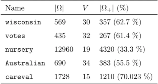
dummy variables, i.e, if a categorical variable with ν levels is present, it will be replaced by ν−1 binary variables. A description of the datasets can be found in Table 1. Such table is split in 4 columns. The first shows the name of the dataset. The total number of samples of the dataset is given in the second one. The number of variables considered, and the number (and percentage) of
195
positive samples in the dataset, are given in the two last columns. Name |Ω| V |Ω+|(%) wisconsin 569 30 357 (62.7 %) votes 435 32 267 (61.4 %) nursery 12960 19 4320 (33.3 %) Australian 690 34 383 (55.5 %) careval 1728 15 1210 (70.023 %)
Table 1: Details concerning the implementation of the CSVM for the considered datasets.
4.2. Results under the cost-sensitive sparse SVM with linear kernel
As commented before, two types of results will be shown here, as in the following subsection. The first one will correspond to the results when Hoeffding
Inequality is not considered (10), whereas the other one consists on the values
200
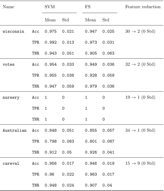
obtained when Hoeffding is used (11). The results will show how the first option leads to more sparsity while the second choice implies a better predictive power. Let us start with the first case, summarized in Table 2.
The first column of Table 2 gives the name of the dataset used. Then, the second and third columns show, respectively, the performance measures for the
205
standard SVM (using the linear kernel) and the proposed cost-sensitive sparse methodology. Such columns are split into two subcolumns: the first one shows the average values and the second one the standard deviations. The last column reports the feature reduction, by indicating the original and selected (average) number of variables. From the table, it can be concluded that the approach
210
with a linear kernel works well in general. In the case of wisconsin, the TPR has desirable values, since it only differentiates -0.019 points from the original. However, in the case of the accuracy and TNR, the loss is bigger than 0.025 points. This is due mainly to two aspects: first, the constraints are forced for the training sample while the performance is calculated using a validation
215
sample. Second, since the thresholds are considered asλ∗1=λ1,λ∗−1=λ−1, this implies we are not much restrictive as if λ∗1 > λ1 (λ∗−1 > λ−1) were required.
Nevertheless, the new TNR value is only 0.038 points smaller than the original, and the reduction of features is significant since only two variables out of 30 are used. Also, invotesthe features are significantly reduced and the most affected
220
performance measure is the TPR, which decreases 0.027 points, which makes the accuracy smaller. However, the value on the TNR is increased. As happened withwisconsin, the loss is due mainly to the two facts previously mentioned. Fornursery, an amazing reduction to only one feature is achieved, in addition getting a perfect classification. This is explained as follows. As commented in
225
Section 4.1, multiclass datasets are transformed into 2-class ones, and this is the case, obtaining the classes “not recom” and “others”, which are the positive and negative classes, respectively. In addition, one of the (categorical) features in the data (which is the one selected by our procedure) completely determines the class. InAustralian, the total number of variables is also reduced to only
Table 2: Performance measures under the cost-sensitive sparse SVM with linear kernel and
λ∗1=λ1,λ∗−1=λ−1.
Name SVM FS Feature reduction
Mean Std Mean Std wisconsin Acc 0.975 0.021 0.947 0.025 30→2 (0 Std) TPR 0.992 0.013 0.973 0.031 TNR 0.943 0.051 0.905 0.063 votes Acc 0.954 0.033 0.949 0.036 32→2 (0 Std) TPR 0.955 0.038 0.928 0.059 TNR 0.947 0.059 0.979 0.036 nursery Acc 1 0 1 0 19→1 (0 Std) TPR 1 0 1 0 TNR 1 0 1 0 Australian Acc 0.848 0.051 0.855 0.057 34→1 (0 Std) TPR 0.798 0.083 0.801 0.087 TNR 0.912 0.05 0.926 0.041 careval Acc 0.956 0.017 0.946 0.019 15→9 (0 Std) TPR 0.96 0.022 0.963 0.017 TNR 0.948 0.024 0.907 0.04
Table 3: Performance measures under the cost-sensitive sparse SVM with linear kernel and
λ∗1=λ1+
p
−logα/(2|I1|),λ∗−1=λ−1+p−logα/(2|I−1|).
Name SVM FS Feature reduction
Mean Std Mean Std wisconsin Acc 0.975 0.021 0.965 0.023 30→6.2 (0.919 Std) TPR 0.992 0.013 0.975 0.023 TNR 0.943 0.051 0.947 0.048 votes Acc 0.954 0.033 0.954 0.033 32→9.3 (1.16 Std) TPR 0.955 0.038 0.96 0.034 TNR 0.947 0.059 0.945 0.052 nursery Acc 1 0 1 0 19→1 (0 Std) TPR 1 0 1 0 TNR 1 0 1 0 Australian Acc 0.848 0.051 0.837 0.057 34→5.75 (1.89 Std) TPR 0.769 0.083 0.772 0.074 TNR 0.912 0.05 0.924 0.053 careval Acc 0.956 0.017 0.954 0.018 15→11 (0 Std) TPR 0.96 0.022 0.962 0.018 TNR 0.948 0.024 0.935 0.039
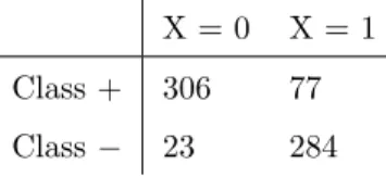
one, having similar performance measures values as in the standard SVM. In fact, we obtain here even better results than under the original linear SVM. If the variable selected with the algorithm is studied, one can observe that it is a binary variable X, where the contingency table together with the class variable is Table 4. Hence this variable is by itself a good predictor, as the FS
235
procedure pointed out. In the case ofcareval, we got the smallest reduction in the number of variables selected, maintaining the performance measures values above the imposed thresholds.
X = 0 X = 1 Class + 306 77 Class− 23 284
Table 4: Contingency table of the feature selected inAustralian.
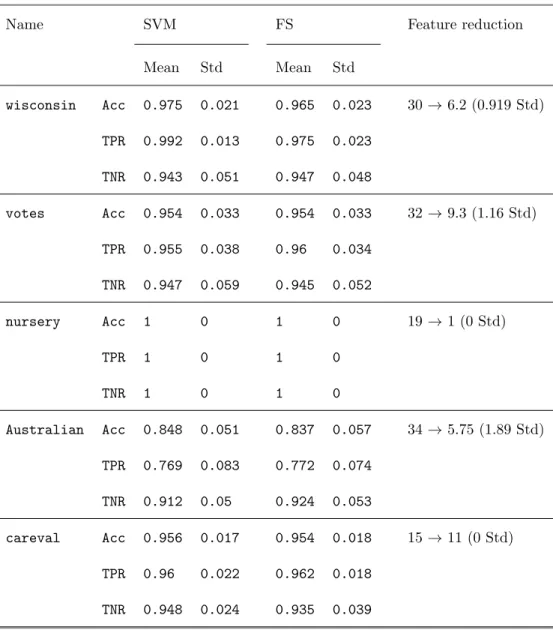
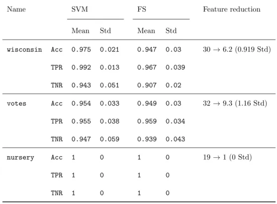
Consider next the results shown by Table 3, for the case where we are restric-tive regarding the performance values, that is, whenλ∗
1=λ1+ p −logα/(2|I1|) 240 andλ∗ −1 =λ−1+ p
−logα/(2|I−1|). From the table, it can be seen how this approach works better concerning the performance measures, but achieves less sparse solutions. For example, if we focus on wisconsin, as much the TNR as the TPR and the accuracy, obtain the desired performance requirements. However, only a reduction of variables of a fifth part is obtained. In the case of
245
votes, an analogous result is obtained for the performance measures and only a reduction in a third part of the variables is achieved. The same pattern as be-fore is observed fornursery. ForAustralian, we obtain even an improvement in all the three performance measures considered, reducing the number of fea-tures to a fifth part. Finally, we get again incarevalthe smallest reduction in
250
the number of variables selected, maintaining the performance measures values above the thresholds imposed as before, but using a larger number of features. 4.3. Results under the cost-sensitive sparse SVM with radial kernel
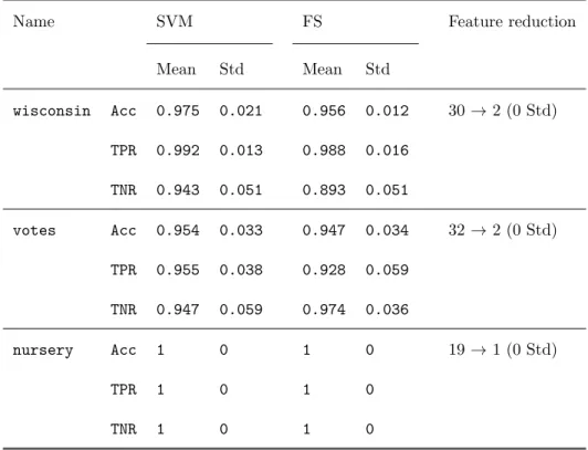
The analogous results to those in Section 4.2 are presented here, for the case of the radial kernel. However, only wisconsin, votes and Australian
datasets are used here. As shown by Tables 5 and 6 and similarly as occurred in Section 4.2, the use of the threshold values obtained by the Hoeffding inequality (as in (11)) lead to a lower level of sparsity, but also, to a higher predictive power in general (particularly, when achieving the desired bounds). Concerning the performance measures, it can be deduced from Tables 5 and 6 that this
260
approach works well in general, especially when using Hoeffding. Finally, it should be noted how the reduction in the number of features is quite notable for some datasets, as before.
Table 5: Performance measures under the cost-sensitive sparse SVM with radial kernel and
λ∗
1=λ1,λ∗−1=λ−1.
Name SVM FS Feature reduction
Mean Std Mean Std wisconsin Acc 0.975 0.021 0.956 0.012 30→2 (0 Std) TPR 0.992 0.013 0.988 0.016 TNR 0.943 0.051 0.893 0.051 votes Acc 0.954 0.033 0.947 0.034 32→2 (0 Std) TPR 0.955 0.038 0.928 0.059 TNR 0.947 0.059 0.974 0.036 nursery Acc 1 0 1 0 19→1 (0 Std) TPR 1 0 1 0 TNR 1 0 1 0
Table 6: Performance measures under the cost-sensitive sparse SVM with radial kernel and λ∗ 1=λ1+ p −logα/(2|I1|),λ∗−1=λ−1+ p −logα/(2|I−1|).
Name SVM FS Feature reduction
Mean Std Mean Std wisconsin Acc 0.975 0.021 0.947 0.03 30→6.2 (0.919 Std) TPR 0.992 0.013 0.967 0.039 TNR 0.943 0.051 0.907 0.02 votes Acc 0.954 0.033 0.949 0.03 32→9.3 (1.16 Std) TPR 0.955 0.038 0.959 0.034 TNR 0.947 0.059 0.939 0.043 nursery Acc 1 0 1 0 19→1 (0 Std) TPR 1 0 1 0 TNR 1 0 1 0
5. Concluding remarks
In this paper we have proposed a Feature Selection procedure for binary
265
Support Vector Machines that yields a novel, sparse, SVM. Contrary to existing Feature Selection approaches, we take explicitly into account that misclassifica-tion costs may be rather different in the two groups, and thus, instead of seeking the classifier maximizing the margin, we seek the most sparse classifier that at-tains certain true positive and true negative rates on the dataset. For both
270
SVM with linear and radial kernel, the problem is written in a straightforward manner, solving first a mixed integer linear problem and then their standard SVM formulations, considering only the features obtained in the first problem as well as the performance constraints. The reported numerical results show that the novel approaches lead to comparable or better performance rates in
275
addition to an important reduction in the number of variables.
Several extensions of the approach presented in this paper are possible and, in our opinion, deserve further study. First, several classification and regression procedures based on optimization problems, such as Support Vector Regres-sion, logistic regression or distance-weighted discrimination, are amenable to
280
address, as done here, an integrated FS and classification or regression. The optimization problems obtained in this way have a structure which should be exploited to make the approach competitive. Second, even within SVM, it should be observed that SVM is a tool for binary classification. For multiclass datasets, classification is performed by solving a series of SVM problems, see
285
[18, 40]. When some classes are hard to identify, the basic multiclass strategies may yield discouraging results. Performing simultaneously feature selection and class fusion, as in [41], is an interesting nontrivial extension of our approach. To do this, problems (P1), (P2) and (P3) will need to be conveniently modified.
Acknowledgements 290
This research is financed by Fundaci´on BBVA, projects FQM329 and P11-FQM-7603 (Junta de Andaluc´ıa, Andaluc´ıa) and MTM2015-65915-R (Ministerio
de Econom´ıa y Competitividad, Spain). The last three are cofunded with EU ERD Funds. The authors are thankful for such support.
Appendix 295
In this section we describe step by step how formulation (9) is built from equation (8). Hence, let us suppose first that we have the model
minw,β,ξ w>w+CPi∈Iξi
s.t. yi(w>xi+β)≥1−ξi, i∈I 0≤ξi≤L(1−ζi) i∈I
µ(ζ)`≥λ` `∈L
ζi∈ {0,1} i∈I. This one can be rewritten as
minζ minω,β,ξ ω>ω+CP i∈I ξi s.t. ζi∈ {0,1} i∈I s.t. yi ω>xi+β ≥1−ξi, i∈I µ(ζ)`≥λ` `∈L 0≤ξi≤L(1−ζi) i∈I If we assume that the binary variablesζfixed, the Karush–K¨uhn–Tucker (KKT) conditions for the inner problem are
ω = P i∈I αiyixi 0 = P i∈I αiyi 0 ≤ αi≤C/2 i∈I.
Substituting these expressions into the last optimization problem, the partial dual of such problem can be calculated, obtaining
300 min ζ α,β,ξmin P i∈I αiyixi > P i∈I αiyixi +CP i∈I ξi s.t. zj∈ {0,1} j∈J s.t. yi P i∈I αiyixi > xi+β ! ≥1−ξi i∈I µ(ζ)`≥λ` `∈L 0≤ξi≤L(1−ζi) i∈I P i∈I αiyi= 0 0≤αi≤C/2 i∈I
As a last step, the kernel trick is used and the final formulation (9) is obtained.
References
[1] D. Bertsimas, A. K. O’Hair, W. R. Pulleyblank, The Analytics Edge, Dy-namic Ideas, Massachusetts, 2016.
[2] F. Provost, T. Fawcett, Data Science for Business: What You Need
305
to Know about Data Mining and Data-Analytic Thinking, 1st Edition, O’Reilly Media, Inc., 2013.
[3] P. L. Bartlett, M. I. Jordan, J. D. McAuliffe, Convexity, classification, and risk bounds, Journal of the American Statistical Association 101 (473) (2006) 138–156.
310
[4] A. Ben-Tal, S. Bhadra, C. Bhattacharyya, J. Saketha Nath, Chance con-strained uncertain classification via robust optimization, Mathematical Programming 127 (1) (2011) 145–173.
[5] R. I. Bot¸, N. Lorenz, Optimization problems in statistical learning: Dual-ity and optimalDual-ity conditions, European Journal of Operational Research
315
213 (2) (2011) 395–404.
[6] P. S. Bradley, U. M. Fayyad, O. L. Mangasarian, Mathematical Program-ming for Data Mining: Formulations and Challenges, INFORMS Journal on Computing 11 (3) (1999) 217–238.
[7] E. Carrizosa, A. Nogales-G´omez, D. Romero-Morales, Strongly agree or
320
strongly disagree?: Rating features in support vector machines, Information Sciences 329 (2016) 256–273.
[8] E. Carrizosa, A. Nogales-G´omez, D. Romero-Morales, Clustering categories in support vector machines, Omega 66 (2017) 28–37.
[9] E. Carrizosa, D. Romero-Morales, Supervised classification and
mathemati-325
[10] D. Corne, C. Dhaenens, L. Jourdan, Synergies between operations research and data mining: The emerging use of multi-objective approaches, Euro-pean Journal of Operational Research 221 (3) (2012) 469–479.
[11] J. S. Marron, M. J. Todd, J. Ahn, Distance-weighted discrimination,
Jour-330
nal of the American Statistical Association 102 (480) (2007) 1267–1271. [12] S. Meisel, D. Mattfeld, Synergies of Operations Research and Data Mining,
European Journal of Operational Research 206 (1) (2010) 1–10.
[13] O. P. Panagopoulos, V. Pappu, P. Xanthopoulos, P. M. Pardalos, Con-strained subspace classifier for high dimensional datasets, Omega 59 (2016)
335
40–46.
[14] F. Plastria, E. Carrizosa, Minmax-distance approximation and separa-tion problems: geometrical properties, Mathematical Programming 132 (1) (2012) 153–177.
[15] P. Richt´arik, M. Tak´aˇc, Parallel coordinate descent methods for big data
340
optimization, Mathematical Programming 156 (1) (2016) 433–484. [16] B. N. S´anchez, M. Wu, P. X. K. Song, W. Wang, Study design in
high-dimensional classification analysis, Biostatistics 17 (4) (2016) 722. doi: 10.1093/biostatistics/kxw018.
[17] X. Shen, G. C. Tseng, X. Zhang, W. H. Wong, Onψ-learning, Journal of
345
the American Statistical Association 98 (463) (2003) 724–734.
[18] N. Cristianini, J. Shawe-Taylor, An Introduction to Support Vector Ma-chines and Other Kernel-based Learning Methods, Cambridge University Press, 2000.
[19] V. Vapnik, The Nature of Statistical Learning Theory, Springer-Verlag New
350
York, Inc., New York, NY, USA, 1995.
[21] H. Aytug, Feature selection for support vector machines using Generalized Benders Decomposition, European Journal of Operational Research 244 (1) (2015) 210–218.
355
[22] P. Bertolazzi, G. Felici, P. Festa, G. Fiscon, E. Weitschek, Integer program-ming models for feature selection: New extensions and a randomized solu-tion algorithm, European Journal of Operasolu-tional Research 250 (2) (2016) 389–399.
[23] P. S. Bradley, O. L. Mangasarian, W. N. Street, Feature Selection via
Math-360
ematical Programming, INFORMS Journal on Computing 10 (2) (1998) 209–217.
[24] E. Carrizosa, B. Mart´ın-Barrag´an, D. Romero-Morales, Detecting relevant variables and interactions in supervised classification, European Journal of Operational Research 213 (1) (2011) 260–269.
365
[25] G. M. Fung, O. L. Mangasarian, A Feature Selection Newton Method for Support Vector Machine Classification, Computational Optimization and Applications 28 (2) (2004) 185–202. doi:10.1023/B:COAP.0000026884. 66338.df.
URLhttp://dx.doi.org/10.1023/B:COAP.0000026884.66338.df
370
[26] I. Guyon, A. Elisseeff, An Introduction to Variable and Feature Selection, Journal of Machine Learning Research 3 (Mar) (2003) 1157–1182.
[27] H. A. Le Thi, H. M. Le, T. P. Dinh, Feature selection in machine learning: an exact penalty approach using a Difference of Convex function Algorithm, Machine Learning 101 (1) (2015) 163–186.
375
[28] S. Maldonado, R. Weber, A wrapper method for feature selection using Support Vector Machines, Information Sciences 179 (13) (2009) 2208–2217. [29] S. Maldonado, R. Weber, J. Basak, Simultaneous feature selection and classification using kernel-penalized support vector machines, Information Sciences 181 (1) (2011) 115–128.
[30] J. Weston, S. Mukherjee, O. Chapelle, M. Pontil, T. Poggio, V. Vapnik, Feature Selection for SVMs, in: T. K. Leen, T. G. Dietterich, V. Tresp (Eds.), Advances in Neural Information Processing Systems 13, MIT Press, 2001, pp. 668–674.
URLhttp://papers.nips.cc/paper/1850-feature-selection-for-svms.
385
[31] S. Ben´ıtez-Pe˜na, R. Blanquero, E. Carrizosa, P. Ram´ırez-Cobo, On Support Vector Machines under a multiple-cost scenario, working Paper (2017). [32] D. Bertsimas, A. King, R. Mazumder, et al., Best subset selection via a
modern optimization lens, The Annals of Statistics 44 (2) (2016) 813–852.
390
[33] D. Bertsimas, R. Mazumder, et al., Least quantile regression via modern optimization, The Annals of Statistics 42 (6) (2014) 2494–2525.
[34] E. Carrizosa, A. V. Olivares-Nadal, P. Ram´ırez-Cobo, A sparsity-controlled vector autoregressive model, Biostatistics (2017) kxw042.
[35] E. Carrizosa, B. Mart´ın-Barrag´an, D. Romero-Morales, Multi-group
sup-395
port vector machines with measurement costs: A biobjective approach, Discrete Applied Mathematics 156 (6) (2008) 950–966.
[36] Gurobi Optimization, Inc., Gurobi optimizer reference manual (2016).
URLhttp://www.gurobi.com
[37] Python Core Team, Python: A dynamic, open source programming
lan-400
guage, Python Software Foundation. (2015).
URLhttps://www.python.org
[38] R. Kohavi, A Study of Cross-Validation and Bootstrap for Accuracy Esti-mation and Model Selection, in: IJCAI, Vol. 14, Stanford, CA, 1995, pp. 1137–1143.
405
[39] M. Lichman, UCI Machine Learning Repository (2013).
[40] L. Wang, X. Shen, On L1-Norm Multiclass Support Vector Machines, Journal of the American Statistical Association 102 (478) (2007) 583–594.
doi:10.1198/016214506000001383.
410
[41] J. Guo, Simultaneous variable selection and class fusion for high-dimensional linear discriminant analysis, Biostatistics 11 (4) (2010) 599.
doi:10.1093/biostatistics/kxq023.