Map Task Scheduling in MapReduce with Data
Locality: Throughput and Heavy-Traffic Optimality
Weina Wang, Kai Zhu and Lei Ying
Electrical, Computer and Energy Engineering Arizona State University
Tempe, Arizona 85287
{weina.wang, kzhu17, Lei.Ying.2}@asu.edu
Jian Tan and Li Zhang
IBM T. J. Watson Research Center Yorktown Heights, New York, 10598
{tanji, zhangli}@us.ibm.com
Abstract—Scheduling map tasks to improve data locality is crucial to the performance of MapReduce. Many works have been devoted to increasing data locality for better efficiency. However, to the best of our knowledge, fundamental limits of MapReduce computing clusters with data locality, including the capacity region and theoretical bounds on the delay performance, have not been studied. In this paper, we address these problems from a stochastic network perspective. Our focus is to strike the right balance between data-locality and load-balancing to simultaneously maximize throughput and minimize delay. We present a new queueing architecture and propose a map task scheduling algorithm constituted by the Join the Shortest Queue policy together with the MaxWeight policy. We identify an outer bound on the capacity region, and then prove that the proposed algorithm stabilizes any arrival rate vector strictly within this outer bound. It shows that the algorithm is throughput optimal and the outer bound coincides with the actual capacity region. Further, we study the number of backlogged tasks under the proposed algorithm, which is directly related to the delay performance based on Little’s law. We prove that the proposed algorithm is heavy-traffic optimal, i.e., it asymptotically minimizes the number of backlogged tasks as the arrival rate vector approaches the boundary of the capacity region. Therefore, the proposed algorithm is also delay optimal in the heavy-traffic regime.
I. INTRODUCTION
Processing large-scale datasets has become an increasingly important and challenging problem as the amount of data cre-ated by online social networks, healthcare industry, scientific research, etc., explodes. MapReduce/Hadoop [1, 2] is a simple yet powerful framework for processing large-scale datasets in a distributed and parallel fashion, and has been widely used in practice, including Google, Yahoo!, Facebook, Amazon and IBM.
A production MapReduce cluster may even consist of tens of thousands of machines [3]. The stored data are typically organized on distributed file systems (e.g., Google File System (GFS) [4], Hadoop Distributed File System (HDFS) [5]), which divide a large dataset into data chunks (e.g.,64MB) and store multiple replicas (by default 3) of each chunk on different machines. A data processing request under the MapReduce framework, called a job, consists of two types of tasks: map and reduce. A map task reads one data chunk and processes it to produce intermediate results (key-value pairs). Then
reduce tasks fetch the intermediate results and carry out further computations to produce the final result. Map and reduce tasks are assigned to the machines in the computing cluster by a master node which keeps track of the status of these tasks to manage the computation process. In assigning map tasks, a critical consideration is to place map tasks on or close to machines that store the input data chunks, a problem called data locality.
For each task, we call a machine a local machine for the task if the data chunk associated with the task is stored locally, and we call this task a local task on the machine; otherwise, the machine is called aremote machinefor the task and correspondingly this task is called a remote task on the machine. The termlocalityis also used to refer to the fraction of tasks that run on local machines. Improving locality can reduce both the processing time of map tasks and the network traffic load since fewer map tasks need to fetch data remotely. However, assigning all tasks to local machines may lead to an uneven distribution of tasks among machines, i.e., some machines may be heavily congested while others may be idle. Therefore, we need to strike the right balance between data-locality and load-balancing in MapReduce.
In this paper, we call the algorithm that assigns map tasks to machines a map-scheduling algorithm or simply a scheduling algorithm. There have been several attempts to increase data locality in MapReduce to improve the system efficiency. For example, the currently used scheduling algorithms in Google’s MapReduce and Hadoop take the location information of data chunks into account and attempt to schedule a map task as close as possible to the machine that has the data chunk [1, 6, 7]. A scheduling algorithm calleddelay scheduling, which delays some tasks for a small amount of time to attain higher locality, has been proposed in [7]. In addition to scheduling algorithms, data replication algorithms such as Scarlett [3] and DARE [8] have also been proposed.
While the data locality issue has received a lot of attention and scheduling algorithms that improve data locality have been proposed in the literature and implemented in practice, to the best of our knowledge, none of the existing works have studied the fundamental limits of MapReduce computing clusters with data locality. Basic questions such as what is the capacity
region of a MapReduce computing cluster with data locality, which scheduling algorithm can achieve the full capacity region,how to minimize the waiting time and congestion in a MapReduce computing cluster with data locality, remain open. In this paper, we will address these basic questions from a stochastic network perspective. Motivated by the observation that a large portion of jobs are map-intensive, and many of them only require map tasks [9], we focus on map scheduling algorithms and assume reduce tasks are either not required or not the bottleneck of the job processing. We assume that the data have been divided into chunks, and each chunk has three replicas stored on three different machines. The computing cluster is modeled as a time-slotted system, in which jobs consisting of a number of map tasks arrive at the beginning of each time slot according to some stochastic process. Each map task processes one data chunk. Within each time slot, a task is completed with probability α at a local machine, or with probability γ (γ < α) at a remote machine, i.e., the service times are geometrically distributed with different parameters. Based on this model, we establish the following fundamental results:
• First, we present an outer bound on the capacity region of a MapReduce computing cluster with data locality, where the capacity region consists of all arrival vectors for which there exists a scheduling algorithm that stabilizes the system (stability region in [10]).
• We propose a new queueing architecture with one local
queue for each machine, storing local tasks associated with the machine, and a common queue for all machines. Based on this new queueing architecture, we propose a two-stage map scheduling algorithm under which a newly arrived task is routed to one of the three queues associated with the three local machines or the common queue using the Join the Shortest Queue (JSQ) policy; and when a machine is idle, it selects a task from the local queue associated with it or the common queue using the MaxWeight policy [11].
• We prove that the joint JSQ and MaxWeight scheduling algorithm is throughput optimal, i.e., it can stabilize any arrival rate vector strictly within the outer bound of the capacity region, which also shows that the outer bound is tight and is the same as the actual capacity region. We remark that existing results on MaxWeight-based scheduling algorithms assume deterministic processing (service) time or geometrically distributed processing time with preemp-tive tasks. To the best of our knowledge, the stability of MaxWeight scheduling with random processing time and nonpreemptive tasks has not been established before. So the proof technique itself is a novel contribution of this paper, and may be extended to prove the stability of MaxWeight scheduling for other applications, in which the service times are geometrically distributed. We remark that recently in [12], the authors studied MaxWeight scheduling for resource allocation in clouds and independently established a similar result with more general service time distributions.
• In addition to throughput optimality, we further study the
number of backlogged tasks, which is directly related to the delay performance based on Little’s law. We prove that under a heavy local traffic condition, the joint JSQ and MaxWeight scheduling algorithm is heavy-traffic optimal, i.e., it asymptotically minimizes the number of backlogged tasks as the arrival rate vector approaches the boundary of the capacity region. Therefore, the proposed algorithm strikes the right balance between data-locality and load-balancing and is both throughput and delay optimal in the heavy-traffic regime. The proof of heavy-traffic optimality follows the Lyapunov drift analysis recently developed in [13]. Heavy-traffic optimality of JSQ only and MaxWeight only have been proved in [13]. In [14], the result has been extended to a joint JSQ and MaxWeight algorithm (in a different context) when servers are homogeneous. In this paper, the machines are heterogeneous due to data locality. The proof of heavy-traffic optimality is a non-trivial application of the drift-based analysis.
II. SYSTEMMODEL
We consider a discrete-time model for a computing cluster withM machines, indexed1,2,· · ·, M. Jobs come in stochas-tically and when a job comes in, it brings a random number of map tasks, which need to be served by the machines. We assume that each data chunk is replicated and placed at three different machines. Therefore, each task is associated with three local machines. It takes longer time for a machine to process a task if the required data chunk is not stored locally since the machine needs to retrieve the data first. Tasks can be classified according to the local machines they associate with. For each task, we assemble the indices of its three local machines in an increasing order into a vector
~ L∈
(m1, m2, m3)∈ {1,2,· · · , M}3, m1< m2< m3 ,
which forms thetypeof the task. The notationm∈~Lindicates that machine m is a local machine for type ~L tasks. Let L
denote the set of the existing types in the cluster andN =|L|.
A. Arrival and Service
Let A~L(t) denote the number of type L~ tasks arriving at the beginning of time slot t. We assume that the arrival process is temporally i.i.d. with arrival rate λ~L. We further assume the arrival processes are bounded. At each machine, the service times of tasks follow geometric distributions. The parameter of the geometric distribution isαfor a task at a local machine, and γ at a remote machine. The service process of a task can be viewed as a sequence of independent trials with success probability α or γ, and the sequence stops once we get a success, i.e., once the task is finished. In this model, we assume the parameters satisfy α > γ. Then the average service time of local tasks is less than that of remote tasks; i.e., 1/α <1/γ. Note thatαand γ characterize the different processing efficiency due to data locality.
B. Task Scheduling Algorithm
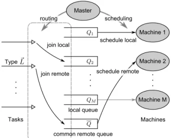
The task scheduling problem is to assign incoming tasks to the machines. Due to data locality, the task scheduling algorithm can significantly affect the efficiency of the sys-tem. In this paper, we consider a task scheduling algorithm consisting of two parts: routing and scheduling. We present a new queue architecture as illustrated in Fig. 1. The master node maintains a queue for each machine m for local tasks, denoted by Qm and called the local queue; and there is a common queue for all machines, denoted byQ(or sometimes QM+1), and called thecommon remote queue. We use a queue
length vectorQ(t) = Q1(t),· · · , QM(t), Q(t)
to denote the queue lengths at the beginning of time slot t. When a task comes in, the master node routes the task to some queue in the queueing system. When a machine is idle, it picks a task from the corresponding local queue or the common remote queue to serve. These two steps are illustrated in Fig. 1. We call the first step routing, and with a slight abuse of terminology we call the second step scheduling. It should be clear from the context that whether we are referring to the whole task scheduling problem or to this service scheduling step. Based on our queue architecture, we propose the following joint routing and scheduling algorithm.
• Join the Shortest Queue (JSQ) Routing. When a task comes in, the master node compares the queue lengths of its three local queues and the common remote queue, and then routes the task to the shortest one. Ties are broken randomly. Let AL,m~ (t) and AL~(t) denote the arrivals of type~Ltasks allocated toQm andQ, respectively. Then the arrivals allocated to each queue can be expressed by the arrival vectorA(t) = A1(t),· · · , AM(t), A(t) , defined as Am(t) =PL~:m∈L~A~L,m(t), m= 1,2,· · ·, M A(t) =P ~ LAL~(t).
• MaxWeight Scheduling. If machinemjust finished a task at time slott−1, then its working status isidle. Otherwise, the machine must be working on some local or remote task. Letfm(t) = 0,1,2denote idle, working on a local task, and working on a remote task, respectively. The working status vector f(t) = (f1(t), f2(t),· · · , fm(t)) and queue length vector Q(t) are reported to the master at the beginning of time slott, and the master makes scheduling decisions for all the machines based onf(t)andQ(t). The idle machines are scheduled according to the MaxWeight algorithm: suppose machinem is idle at time slott, then it serves a local task if αQm(t) ≥ γQ(t) and a remote task otherwise. Other machines continue to serve the unfinished tasks, i.e., the execution of tasks is non-preemptive. Letσm(t) denote the scheduling decision of machinem at time slot t, then it is a function of Q(t)andfm(t), and
σm(t) =
(
1 if a local task is to be served, 2 if a remote task is to be served.
Machine M . . . . . . . . .
join local schedule local
schedule remote scheduling routing
Tasks
common remote queue local queue Type Master join remote Machine 2 Machine 1 Machines
Fig. 1: The Queue Architecture and Scheduling Algorithm
Note thatσm(t)indicates which queue machinemis sched-uled to serve. It can only take value1or2since the machine is scheduled to serve either a local task or a remote task. If machine m is not idle, i.e., fm(t) = 1 or 2, the schedule σm(t)equals tofm(t)by our settings. However if machine mis idle, i.e.,fm(t) = 0,σm(t)is still either1or2, decided by the master according to the MaxWeight algorithm. We use the schedule vectorσ(t) = (σ1(t), σ2(t),· · ·, σM(t))to denote the scheduling decisions of all the machines. Here we note that each queue in this architecture can actually be divided into multiple subqueues according to the job that the task comes from, i.e., per job subqueues. Then in the scheduling step, an idle machine can further pick a subqueue to serve for the fairness purpose. However, this change will not affect our analysis throughout this paper, so we only consider this structure in the simulation part.
C. Queue Dynamics
In time slot t, first the master checks the working status information f(t) and the queue length Q(t). Then the tasks arrive at the master and the master does the routing and the scheduling, yieldingA(t)andσ(t). Define
(
µl
m(t) =α, µrm(t) = 0 ifσm(t) = 1, µl
m(t) = 0, µrm(t) =γ ifσm(t) = 2.
The service from machine m to local queue Qm and re-mote queue Q are two Bernoulli random variables Sl
m(t) ∼ Bern µl
m(t)
and Sr
m(t) ∼ Bern(µrm(t)). Hence the service applied to each queue can be expressed by the service vector S(t) = Sl 1(t),· · ·, SMl (t), PM m=1S r m(t)
, which is the ser-vice process we introduced in Section II-A with serser-vice rateα or γ. Then the queue lengths satisfy the following equations.
• Local queues.For any m= 1,2,· · ·, M,
where Um(t) = ( 0 if Qm(t) +Am(t)≥1, Sl m(t) if Qm(t) +Am(t) = 0.
• The Remote queue.
Q(t+ 1) =Q(t) +A(t)−PM m=1S r m(t) +U(t), where U(t) =PM m=1S r m(t)− P m∈A(t)S r m(t)
andA(t)is the set of machines which actually have some tasks to serve from the remote queue at time slot t. Note that there can be some machines which attempt to serve the remote queue but fail due to insufficient tasks.
By our notations, the queue dynamics can thus be written as
Q(t+ 1) =Q(t) +A(t)−S(t) +U(t), (1) whereU(t) = U1(t),· · ·, UM(t), U(t)
is the unused service. In the case that the service time is deterministic, the queue-ing process {Q(t), t≥0} itself is a Markov chain. However, the service time in our model is random and heterogeneous due to data locality. Thus we need to also consider the working status vectorf(t), andQ(t)together withf(t)forms a Markov chain {(Q(t), f(t)), t≥0}. We assume the initial state is Q(0), f(0)
= 0(M+1)×1,0M×1and the state space S ⊆NM+1× {0,1,2}M consists of all the states which can be reached from the initial state, whereNis the set of nonnegative
integers. Then this Markov chain is irreducible and aperiodic.
III. THROUGHPUTOPTIMALITY
In this section, we first identify an outer bound of the capacity region of the system. We then prove that the proposed task scheduling algorithm stabilizes any arrival rate vector strictly within this outer bound, which means that the proposed algorithm isthroughput optimal, and the capacity region coin-cides with the outer bound.
A. Capacity Region
For any task type L~ ∈ L, we assume that the number of typeL~ arrivals allocated to machinem has a rateλL,m~ , then λ~L =
PM
m=1λL,m~ . The set of rates
λL,m~ L~∈L,m=1,···,M will be called a decomposition of the arrival rate vector λ = λ~L1, λL~2,· · · , λLN~
in the rest of this paper, and the index range may be omitted for conciseness. For any machine m, a necessary condition for an arrival rate vector λ to be supportable is that the average arrivals allocated to machinem in one time slot can be served within one time slot, i.e.,
X ~ L:m∈L~ λL,m~ α + X ~ L:m /∈L~ λL,m~ γ ≤1, (2)
where the left hand side is the time machinemneeds to serve the arrivals allocated to it in one time slot on average, since the service rate isαfor local tasks andγ for remote tasks.
LetΛ be the set of arrival rates such that each element has a decomposition satisfying (2). Formally,
Λ = λ= λL~1, λL~2,· · ·, λL~N : λ~L= M X m=1 λL,m~ , ∀~L∈ L, (3) λ~L,m≥0, ∀L~ ∈ L, ∀m= 1,· · · , M X ~ L:m∈L~ λL,m~ α + X ~ L:m /∈L~ λL,m~ γ ≤1, ∀m= 1,· · ·, M . ThenΛ gives an outer bound of the capacity region.
B. Achievability
Theorem 1 (Throughput Optimality). The proposed map-scheduling algorithm stabilizes any arrival rate vector strictly within Λ. Hence, this algorithm is throughput optimal, andΛ is the capacity region of the system.
We give the outline of the proof below due to space limit, and refer to our technical report [15] for the complete proof.
Proof Outline: Since {(Q(t), f(t)), t≥0} is an irre-ducible and aperiodic Markov chain, the stability is defined to be the positive recurrence of this Markov chain. By the extension of the Foster-Lyapunov theorem, it is sufficient to find a positive integer T and a Lyapunov function whose T time slot Lyapunov drift is bounded within a finite subset of the state space and negative outside this subset.
Step 1.Consider the Lyapunov function
W(Q(t), f(t)) =kQ(t)k2=PM m=1Q 2 m(t) +Q 2 (t). The Lyapunov drift from time slott0tot0+T is bounded by
2EhPt0+T−1 t=t0 hQ(t), A(t)−S(t)i Q(t0), f(t0) i +const. (4)
Step 2. Consider an arrival process with arrival rate vector λ= λ~L1,· · · , λ~LN ∈Λoand defineλ˜= ˜λ1,· · · ,λ˜M+1 as ˜ λm=PL~:m∈L~λ~L,m, m= 1,2,· · ·, M, ˜ λM+1 =P M m=1 P ~ L:m /∈L~λ~L,m. Then we can write the expectation in bound (4) as
E h Pt0+T−1 t=t0 hQ(t), A(t)−S(t)i Q(t0), f(t0) i =E h P t hQ(t), A(t)i − hQ(t),˜λi Q(t0), f(t0) i (5) +EhP t hQ(t),λ˜i − hQ(t), S(t)i Q(t0), f(t0) i . (6)
Step 3.The arrival part (5) under the JSQ routing is bounded by Lemma 8 in our technical report [15] as,
E h P t hQ(t), A(t)i − hQ(t),˜λi Q(t0), f(t0) i ≤0. Step 4. To bound the service part (6), we start with the following random variables
t∗m= min{τ:τ≥t0, fm(τ) = 0}, m= 1,2,· · ·, M, t∗= max 1≤m≤Mt ∗ m. (7)
Thus t∗m is the first time slot after t0 at which machinem is
idle and makes a scheduling decision, and t∗ is the first time slot by which every machine has been idle for at least once since t0. We use t∗ to decompose the probability space. Let
T =J K, then E h P t hQ(t),˜λi − hQ(t), S(t)i Q(t0), f(t0) i =EhP t hQ(t),˜λi − hQ(t), S(t)i Q(t0), f(t0), (8) t∗≥t0+K i ·Pr (t∗≥t0+K|Q(t0), f(t0)) +E h P t hQ(t),λ˜i − hQ(t), S(t)i Q(t0), f(t0), (9) t∗< t0+K i ·Pr (t∗< t0+K|Q(t0), f(t0)).
Step 4a.For term (8), by boundedness of arrival and service,
E h P t hQ(t),˜λi − hQ(t), S(t)i Q(t0), f(t0), t∗≥t0+K i ≤T M QΣ(t0) +const, whereQΣ=P M
m=1Qm+Qdenote the queue length sum. Step 4b. For term (9), we further condition on t∗. For the summation fromt=t0tot∗, under the conditiont∗< t0+K,
Pt∗ t=t0E h hQ(t),λ˜i − hQ(t), S(t)i t∗, Q(t0), f(t0) i ≤KM QΣ(t0) +const.
For the summation fromt=t∗+ 1 tot
0+T −1, first since
λ∈Λo, there exists >0 and a decomposition
λ~L,m such that X ~ L:m∈L~ λL,m~ α + X ~ L:m /∈L~ λL,m~ γ ≤ 1 1 +. (10) Thus Qm(t)P ~ L:m∈~LλL,m~ +Q(t)PL~:m /∈L~λL,m~ ≤ 1 1 +max αQm(t), γQ(t) . Next consider the random variableτt
m defined as
τmt = max{τ:τ≤t, fm(τ) = 0}, m= 1,2,· · ·, M, (11) which is the last time slot before t at which machine m is idle and is scheduled to some queue based on the MaxWeight algorithm. Thus for eachtsuch thatt∗< t≤t0+T, we have
t0≤τmt ≤t0+T. By the MaxWeight algorithm,
Qm(τmt)ESml (t) σm(τmt) +Q(τmt)ESmr(t) σm(τmt) = ( αQm(τmt) if σm(τmt) = 1, i.e., if αQm(τmt)≥γQ(τmt) γQ(τt m) if σm(τmt) = 2, i.e., if αQm(τmt)≤γQ(τmt) ≥max αQm(τmt), γQ(τ t m) .
Then utilizing conditional expectations and the bounded dif-ference between any two ofQ(τt
m),Q(t) andQ(t0), yields Pt0+T t=t∗+1E h hQ(t),λ˜i − hQ(t), S(t)i t ∗, Q(t 0), f(t0) i ≤ − (J−1)KαγM (1 +)(γM+α)QΣ(t0) +const.
Combining the two summations gives
E h P t hQ(t),˜λi − hQ(t), S(t)i Q(t0), f(t0), t∗< t0+K i ≤KM 1− (J−1)αγ (1 +)(γM+α) QΣ(t0) +const.
Step 4c. We show that Pr (t∗≥t0+K|Q(t0), f(t0)) → 0
asK→ ∞in Lemma 10 of our technical report [15]. Choose large enough K and J, i.e., large enough T, then for some θ >0, E h P t hQ(t),λ˜i − hQ(t), S(t)i Q(t0), f(t0) i ≤ −θQΣ(t0) +const.
Step 5.TheT time slot Lyapunov drift fromt0is thus bounded
as D(Q(t0), f(t0))≤ −2θQΣ(t0) +B for a constant B >0.
Step 6.LetB=
(Q, f)∈ S:Q1+· · ·+QM+1≤B2+θδ for
an arbitraryδ >0. ThenBis a finite subset ofSsatisfying that for any (Q, f)∈ Bc, D(Q, f)≤ −δ and for any (Q, f)∈ B, D(Q, f) ≤B. This finishes the proof for stability. Thus the proposed task scheduling algorithm is throughput optimal, and Λ is the capacity region of the system.
IV. HEAVY-TRAFFICOPTIMALITY
In this section, we analyze the performance of the proposed algorithm beyond throughput. We will show that in the heavy-traffic regime, the proposed algorithm asymptotically mini-mizes the number of backlogged tasks.
Suppose the set of existing task typesLis such that there are Ml machines, each of which is considered as a local machine by some task type, and the otherMr=M−Mlmachines are remote machines for all the task types. Denote the set of the machines which can have local tasks asMl and the set of the machines which only have remote tasks as Mr. Then
Ml=
m∈ {1,2,· · · , M}:∃L~ ∈ L, s.t.m∈~L ,
Mr={1,2,· · · , M} − Ml,
and|Ml|=Ml,|Mr|=Mr. Without loss of generality, we assumeMl={1,· · · , Ml} andMr={Ml+ 1,· · · , M}.
We consider the heavy-traffic regime that the arrival rates satisfy that for any subsetHofMl, the sum arrival rate of local tasks to the machines inHis larger than the process capacity of the machines. Formally, let λ= λL~1,· · ·, λLN~
∈Λo be the arrival rate vector, then we assume for anyH ⊆ Ml,
X
~
L:∃m∈H,s.t.m∈~L
λL~ ≥ |H|α, (12)
which is referred to as the heavy local traffic assumption. In this regime, the machines inMlcannot accommodate the local arrivals, so we assumeMr>0 to stabilize the system.
Now if λ is in the capacity region, it is easy to see that
P ~ L∈LλL~ ≤Mlα+Mrγ. We assume that P ~ L∈LλL~ =Mlα+Mrγ−, (13) where >0characterizes the distance between the arrival rate vector and the capacity boundary. The superscript()is used in
Machine
Arrival Queue length Service
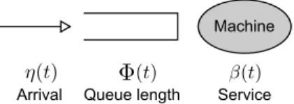
Fig. 2: Lower-Bounding System
this section to indicate the heavy-traffic parameter. Consider any arrival processes
A(~)
L (t), t ≥ 0 L~∈L with arrival rate
vector λ()=λ(~) L1 , λ(~) L2 ,· · ·, λ(~) LN satisfying (13). Then E h P ~ LA () ~ L (t) i =P ~ Lλ () ~ L =Mlα+Mrγ−. The variance of the number of overall arrivals is given by
VarP ~ LA () ~ L (t) = (σ())2.
Denote the queueing and the working status process with such arrival processes as
Q()(t), f()(t)
, t≥0 . Later we will let go to zero to get theheavy-traffic limit.
A. Lower Bound
In this subsection, we derive a lower bound on the expecta-tion of the sum of the queue lengths in steady state. Consider a single server queueing system as depicted in Fig. 2. By properly choosing the arrival and the service process, the queue length in this system is stochastically smaller than the sum of the queue lengths in MapReduce. We refer to this single server system as the lowering bounding system and the task scheduling system in MapReduce as the original system. A lower bound on the expectation of the queue length in steady state in this system is obtained in [13], which is also a lower bound for the original system. Note that this lower bound does not need the heavy local traffic assumption.
Consider the following arrival process η()(t), t≥0 and
service process {β(t), t≥0}: η()(t) =P ~ LA () ~ L (t), β(t) = PMl i=1Xi(t) + PMr j=1Yj(t),
where all the processes {Xi(t), t≥0}, i = 1,· · ·, Ml and
{Yj(t), t≥0}, j = 1,· · · , Mr are independent and each process is composed of a sequence of i.i.d. random variables. Let Xi(t)∼Bern(α) andYj(t) ∼Bern(γ). Then E[β(t)] =
Mlα+Mrγ, and we useν2 to denote Var(β(t)).
By these settings, the queue length Φ()(t) in the lower-bounding system is stochastically smaller than the sum of the queue lengths in the original system for any time slot t. Considering the lower bound on EΦ()(t) in steady state
given by Lemma 4 in [13], we obtain the following theorem.
Theorem 2 (Lower Bound). For the map task scheduling system in MapReduce, consider any arrival process such that the number of total arrivals at each time slot has expectation Mlα+Mrγ− and variance (σ())2. Suppose the Markov chain Q()(t), f()(t)
, t≥0 is in steady state under the proposed map-scheduling algorithm. Then, for anyt and any
such that0 < < Mlα+Mrγ, the expectation of the sum of the queue lengths in steady state can be lower-bounded as
E "M+1 X m=1 Q(m)(t) # ≥(σ ())2+ν2+2 2 − M 2 . (14)
Therefore, in the heavy-traffic limit as the arrival rate ap-proaches the service rate from below, assuming the variance (σ())2 converges to a constantσ2, the lower bound becomes
lim inf →0+ E "M+1 X m=1 Q(m)(t) # ≥σ 2+ν2 2 . (15)
B. State Space Collapse
For a single server queueing system like the one in Fig. 2, the discrete-time Kingman’s bound [16] gives an upper bound on the expectation of the queue length in steady state, which is derived by studying the drift of an appropriate Lyapunov function in steady state. The task scheduling system in MapRe-duce is a more complicated queueing system, which consists of multiple queues and thus has a multi-dimensional state space. However, in the heavy-traffic scenario, we will show that the multi-dimensional state description of the system reduces to a single dimension in the sense that the deviation from a particular direction has bounded moments, independent of the heavy-traffic parameter. This behavior of the queueing system in heavy-traffic scenario is calledstate space collapse. When the state space collapse happens, the system can be analyzed by the similar techniques as used for the single-dimensional system. In this subsection, we will establish the state space collapse for the task scheduling system in MapReduce.
In our model, Q()(t), f()(t)
, t≥0 is an irreducible, aperiodic, positive recurrent Markov chain with state spaceS. Since the working status vector f is always finite, we only consider the subspace for the queue lengths. Let c ∈ RM+1
+
be a vector with unitl2 norm, then the corresponding parallel
and perpendicular components of a queue length vectorQare
Qk=hQ, cic, Q⊥=Q−Qk.
Throughout this paper, the normk·krefers tol2norm. If all the
moments ofkQ⊥k, which represent the deviation of the queue
length vector from the direction c, are bounded by constants not depending on the heavy-traffic parameter , we will say that the state space collapses to the direction of c.
Let c= √ 1 Ml+ 1 (1,· · ·,1 | {z } Ml ,0,· · ·,0 | {z } Mr ,1) (16)
be the direction that we will prove the state space collapses to, where the firstMl entries are ones and the following Mr entries are zeros. Consider the Lyapunov function
V⊥((Q, f)) =kQ⊥k.
We can prove that the drift of V⊥ satisfies the conditions in
Lemma 1 of [13] (see [17] for the derivation of this lemma). Then by this lemma, V⊥ (Q()(t), f()(t) has bounded
Theorem 3 (State Space Collapse). For the map-scheduling system in MapReduce, consider any arrival process with an arrival rate vector strictly within the capacity region sat-isfying the heavy local traffic assumption, and the number of total arrivals at each time slot has expectation Mlα+ Mrγ − and variance (σ())2. Suppose the Markov chain
Q()(t), f()(t)
, t≥0 is in steady state under the pro-posed map-scheduling algorithm. Then for any t and any such that 0< <min Mlα+Mrγ, Mr(Ml+ 1)γ, (Ml+ 1)α 2N , (Ml+ 1) min~L∈LλL~ 6 , there exists a sequence of finite numbers {C1, C2,· · · } such
that for each positive integerr,
E h
kQ(⊥)(t)kri≤C r,
where the ⊥component is w.r.t. the direction defined in(16). The proof of this theorem is omitted here due to space limit, and available in our technical report [15].
C. Upper Bound and Heavy-Traffic Optimality
In this subsection, we derive an upper bound on the expecta-tion of the sum of the queue lengths in steady state based on the Lyapunov drift-based moment bounding techniques developed in [13], and we show that this upper bound is asymptotically tight under the heavy-traffic regime. The heavy-traffic optimal-ity of joint JSQ and MaxWeight algorithm with homogeneous servers has been established in [14] (in a different context). Due to data locality, our system has heterogeneous servers, which makes the problem more challenging.
We have established the state space collapse for the task scheduling system in MapReduce under the proposed algo-rithm, so the queue length vector in steady state concentrates along a single direction. Enlightened by the way how the queue length in the single server queueing system is bounded, we treat the multi-dimensional state space in our problem as a one-dimensional state space along the collapse direction and then set the drift of the Lyapunov functionWk((Q, f)) =kQkk2to
zero in steady state to obtain an upper bound for the expected queue length along this direction.
Due to the different service rates in our system, the terms related to service in the Lyapunov drift cannot be bounded directly. We consider the ideal service process
S0(t) = S10(t),· · · , SM0 +1(t)
, t≥0 , which makes the best use of every machine and is defined as
Sm0 (t) = Xml (t) ifm∈ Ml 0 ifm∈ Mr P m∈MrX r m(t) ifm=M + 1 where all the processes Xl
m(t), t≥0 , m ∈ Ml and
{Xr
m(t), t≥0}, m ∈ Mr are independent and each process is composed of a sequence of i.i.d. random variables. Let
Xl
m(t) ∼ Bern(α) and Xmr(t) ∼ Bern(γ). Utilizing this service process, the queue dynamics (1) can be rewritten as
Q(t+ 1) =Q(t) +A(t)−S0(t) +U0(t), (17) where U0(t) = S0(t)− S(t) + U(t). Since the moments of S0(t) are easy to calculate, we will use this equivalent queue dynamics to express the Lyapunov drift. Then setting the Lyapunov drift to zero gives the following lemma.
Lemma 1. For the map task scheduling system in MapReduce, consider any arrival process with an arrival rate vector strictly within the capacity region. Suppose the queueing process is in steady state at time slottunder the proposed map-scheduling algorithm, then for any directionc,
2E[hc, Q(t)ihc, S0(t)−A(t)i]
=Ehc, A(t)−S0(t)i2+Ehc, U0(t)i2 (18)
+ 2E[hc, Q(t) +A(t)−S0(t)ihc, U0(t)i]. (19) The formal proof of this lemma is provided in our technical report [15]. Analyzing each term in this lemma gives the following upper bound, which is asymptotically tight under the heavy-traffic limit. A more detailed proof of the following theorem is also available in our technical report [15].
Theorem 4(Upper Bound). For the map-scheduling system in MapReduce, consider any arrival process with an arrival rate vector strictly within the capacity region satisfying the heavy local traffic assumption, and the number of total arrivals at each time slot has expectationMlα+Mrγ− and variance (σ())2. Suppose the Markov chain
Q()(t), f()(t)
, t≥0 is in steady state under the proposed map-scheduling algo-rithm. Then for anyt and anysuch that
0< <min Mlα+Mrγ, Mr(Ml+ 1)γ, (Ml+ 1)α 2N , (Ml+ 1) minL~∈Lλ~L 6 , (20)
the expectation of the sum of the queue lengths in steady state can be upper bounded as
E "M+1 X m=1 Q(m)(t) # ≤(σ ())2+ν2 2 +B (), (21) whereB()=o(1 ), i.e., lim →0+B ()= 0.
Therefore, in the heavy-traffic limit as the arrival rate approaches the service rate from below, assuming the variance (σ())2 converges to a constantσ2 the upper bound becomes
lim sup →0+ E "M+1 X m=1 Q(m)(t) # ≤σ 2+ν2 2 . (22)
This upper bound under heavy-traffic limit coincides with the lower bound (15), which establishes the first moment heavy-traffic optimality of the proposed algorithm.
Proof:Fix anthat satisfies (20) and then we temporarily omit the superscript()for simplicity. Since we will study the
performance in steady state, we assume that the Markov chain
{(Q(t), f(t)), t≥0} is in steady state from time slot 0 and consider the equation in Lemma 1 for any t ≥ 0 with the collapse direction cdefined in (16).
First, by the definition of S0(t) and the property of steady
state, the term on the left side of (18) satisfies
E[hc, Q(t)ihc, S0(t)−A(t)i] = Ml+ 1E h PM+1 m=1Qm(t) i . Next, we study the two terms on the right side in (18). Recall the definition of ν2 in the lower-bounding system. Then
Ehc, A(t)−S0(t)i2=
1 Ml+ 1
(σ())2+ν2+2.
For the other termEhc, U0(t)i2, sinceQ(t)is in steady state, E[hc, A(t)−S0(t) +U0(t)i] =E[hc, Q(t+ 1)−Q(t)i] = 0. Therefore E[hc, U0(t)i] =E[hc, S0(t)−A(t)i] = √ Ml+ 1 Ehc, U0(t)i2≤ √ M Ml+ 1 E[hc, U0(t)i] = M Ml+ 1 . Finally we bound the term (19). To bound the expectation of hc, Q(t)ihc, U0(t)i, we write it as
hc, Q(t)ihc, U0(t)i=hQ(t), U0(t)i − hQ⊥(t), U⊥0(t)i
=hQ(t), S0(t)−S(t)i+hQ(t), U(t)i − hQ⊥(t), U⊥0(t)i.
In the case that the service time is deterministic, Q(t) and U0(t)are orthogonal, so we can directly apply the state space collapse result to boundhQ⊥(t), U⊥0 (t)i. However, the service
time in our model is random. To bound hQ(t), U0(t)i with a small number, we start from the following inequality,
E[hQ(t), S0(t)−S(t)i]≤R1 p
Ml+ 1E[hc, S0(t)−S(t)i],
where R1 > 0 is a constant. We sketch the proof of this
inequality as follows and refer to Lemma 17 in our technical report [15] for details. First we expand the inner product and see that it is sufficient to show that for any m∈ Ml,
EQm(t) Xml (t)−S l m(t) +Q(t) (−Smr(t)) ≤R1EXml (t)−S l m(t) . Then we use Q(t), f(t)
to decompose the probability space. For the case fm(t) = 0, machine m makes a scheduling decision at the current time slot, so the inequality follows from the MaxWeight policy. The proof for the casefm(t) = 1 is straightforward since the actual service has the same dis-tribution as the ideal service. For the case fm(t) = 2, we still considerτmt defined in (11). Decomposing the probability space further by the random variable τmt and utilizing the MaxWeight policy and the boundedness of arrival and service yield E h Qm(t) Xml (t)−S l m(t) +Q(t) (−Smr(t)) τ t m=t−n, Q(t) =Q, f(t) =f i ≤n(N Amaxα+M γ).
By the geometric distribution of the service time, the proba-bilityPr (τt
m=t−n|Q(t) =Q, f(t) =f)is proportional to (1−γ)n−1. Thus the conditional expectation over the subspace fm(t) = 2is bounded by a constant timesP∞
n=1n(1−γ)
n−1,
which is also bounded by a constant, and then the inequality follows for proper coefficientR1. Integrating these three cases
gives the inequality we want to prove. This inequality indicates that the MaxWeight algorithm results in a small difference between the actual serviceS(t)and the ideal service S0(t)in the sense that the queue length vectorQ(t)has finite projection in the direction S0(t)−S(t)on average. Now by definitions,
hQ(t), U(t)i=Q(t)U(t)≤M U(t)≤MpMl+ 1hc, U(t)i. LetR2= max{R1, M}>0, then
E[hQ(t), S0(t)−S(t)i+hQ(t), U(t)i] ≤R2 p Ml+ 1E[hc, S0(t)−S(t)i+hc, U(t)i] =R2 p Ml+ 1E[hc, U0(t)i] =R2.
To bound the term −hQ⊥(t), U⊥0(t)i, we use the state space
collapse theorem, which claims that there exists a constant C2 such that EkQ⊥(t)k2 ≤ C2. Then using the
Cauchy-Schwartz inequality and this bound yields,
E[−hQ⊥(t), U⊥0(t)i]≤
q
E[kQ⊥(t)k2]E[kU⊥0(t)k2]
≤pC2E[kU0(t)k2]≤pC 2M .
Meanwhile, the number of arrivals in each time slot is bounded. Thus the term (19) can be bounded as
E[hc, Q(t) +A(t)−S0(t)ihc, U0(t)i] ≤ R2+ N Amax Ml+ 1 +pC2M .
We revive the superscript()now. Combining the inequalities
for the terms in the equation in Lemma 1 yields
E "M+1 X m=1 Q(m)(t) # ≤(σ ())2+ν2 2 +B (), where B()= 2+ M 2 + (Ml+ 1)R2+N Amax+ (Ml+ 1) r C2M .
Obviously lim→0+B() = 0, thus B() = o 1
. Then the bound (22) for the heavy-traffic limit follows immediately by taking limits on both sides.
V. SIMULATIONS
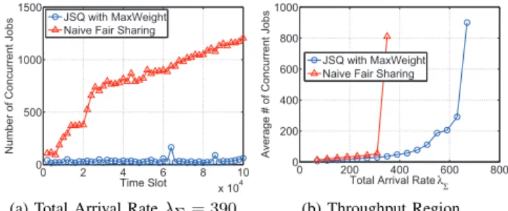
In this section, we use simulations to compare the throughput and delay performance of the proposed algorithm with the na¨ıve fair sharing algorithm proposed in [7]. The na¨ıve fair sharing shows a great performance improvement over the Hadoop’s FIFO scheduler according to the evaluation in [7]. The related simulation parameters are from mimicking real workload analyzed in [18].
0 2 4 6 8 10 x 104 0 500 1000 1500 Time Slot
Number of Concurrent Jobs
JSQ with MaxWeight Naive Fair Sharing
(a) Total Arrival RateλΣ= 390
0 200 400 600 800 0 200 400 600 800 1000
Total Arrival Rate λΣ
Average # of Concurrent Jobs
JSQ with MaxWeight Naive Fair Sharing
(b) Throughput Region
Fig. 3: Throughput Performance
0 200 400 600 800 0 50 100 150 200 250
Total Arrival Rate λΣ
Average Job Delay
JSQ with MaxWeight Naive Fair Sharing
(a) Job Delay in Steady State
0 200 400 600 800 0 1000 2000 3000 4000 5000
Total Arrival Rate λΣ
Average Task Delay
JSQ with MaxWeight Naive Fair Sharing
(b) Task Delay in Steady State
Fig. 4: Delay Performance.
We consider a computing cluster with1000machines and a dataset distributed uniformly in800 of the them. The service rates for local and remote tasks are α = 0.8 and γ = 0.2, respectively, so we only consider the total task arrival rateλΣ
less than 800α+ 200γ = 680 per time slot. For eachλΣ we
simulate the system for one sample path. As noted in Section II, we maintain multiple subqueues for each queue, and the subqueue corresponding to the job with the fewest running tasks is selected during scheduling, as in the na¨ıve fair sharing. Throughput Performance. We keep track of the number of concurrent jobs in the system to observe stability. Fig. 3a shows a representative sample of the evolution of this number over time, indicating the comparison of instability and stability. Fig. 3b shows the average number of concurrent jobs over the last 250,000 time slots for each λΣ. The turning points at
350 and 630 indicate the throughput difference. From these results we can conjecture that the proposed algorithm achieves the maximum throughput, and the throughput is increased by more than80% compared with the na¨ıve fair sharing.
Delay Performance.For eachλΣ, we calculate the average
delay for jobs and tasks departing in steady state and illustrate the results in Fig. 4. We did not plot the results for λΣ ≥
390 under the na¨ıve fair sharing and for λΣ= 670under the
proposed algorithm since the delay becomes very large (more than ten times larger) due to instability, which also confirms the throughput difference of the two algorithms. For small arrival rates, the proposed algorithm roughly halves the average job delay compared with the na¨ıve fair sharing (Fig. 4a), while the average task delay are roughly the same (Fig. 4b).
VI. CONCLUSION
We considered map scheduling algorithms in MapReduce with data locality. We first presented the capacity region of a MapReduce computing cluster with data locality and then we proved the throughput optimality. Beyond throughput, we showed that the proposed algorithm asymptotically minimizes the number of backlogged tasks as the arrival rate vector approaches the boundary of the capacity region, i.e., it is heavy-traffic optimal.
ACKNOWLEDGEMENT
Research supported in part by NSF Grants ECCS-1255425.
REFERENCES
[1] J. Dean and S. Ghemawat, “Mapreduce: simplified data processing on large clusters,”ACM Commun., vol. 51, no. 1, pp. 107–113, Jan. 2008. [2] “Hadoop,” http://hadoop.apache.org.
[3] G. Ananthanarayanan, S. Agarwal, S. Kandula, A. Greenberg, I. Stoica, D. Harlan, and E. Harris, “Scarlett: coping with skewed content popular-ity in mapreduce clusters,” inProc. European Conf. Computer Systems (EuroSys), Salzburg, Austria, 2011, pp. 287–300.
[4] S. Ghemawat, H. Gobioff, and S.-T. Leung, “The google file system,” in
Proc. ACM Symp. Operating Systems Principles (SOSP), Bolton Landing, NY, 2003, pp. 29–43.
[5] K. Shvachko, H. Kuang, S. Radia, and R. Chansler, “The hadoop distributed file system,” in IEEE Symp. Mass Storage Systems and Technologies (MSST), Incline Villiage, NV, May 2010, pp. 1–10. [6] T. White,Hadoop: The definitive guide. Yahoo Press, 2010. [7] M. Zaharia, D. Borthakur, J. Sen Sarma, K. Elmeleegy, S. Shenker, and
I. Stoica, “Delay scheduling: a simple technique for achieving locality and fairness in cluster scheduling,” inProc. European Conf. Computer Systems (EuroSys), Paris, France, 2010, pp. 265–278.
[8] C. Abad, Y. Lu, and R. Campbell, “DARE: Adaptive data replication for efficient cluster scheduling,” inIEEE Int. Conf. Cluster Computing (CLUSTER), Austin, TX, 2011, pp. 159–168.
[9] S. Kavulya, J. Tan, R. Gandhi, and P. Narasimhan, “An analysis of traces from a production mapreduce cluster,” in Proc. IEEE/ACM Int. Conf. Cluster, Cloud and Grid Computing (CCGRID), Melbourne, Australia, 2010, pp. 94–103.
[10] L. Tassiulas and A. Ephremides, “Stability properties of constrained queueing systems and scheduling policies for maximum throughput in multihop radio networks,”IEEE Trans. Autom. Control, vol. 4, pp. 1936– 1948, Dec. 1992.
[11] ——, “Dynamic server allocation to parallel queues with randomly varying connectivity,” IEEE Trans. Inf. Theory, vol. 39, pp. 466–478, Mar. 1993.
[12] S. T. Maguluri and R. Srikant, “Scheduling jobs with unknown duration in clouds,” inProc. IEEE Int. Conf. Computer Communications (INFO-COM), Turin, Italy, 2013.
[13] A. Eryilmaz and R. Srikant, “Asymptotically tight steady-state queue length bounds implied by drift conditions,”Queueing Syst., vol. 72, no. 3-4, pp. 311–359, Dec. 2012.
[14] S. T. Maguluri, R. Srikant, and L. Ying, “Heavy traffic optimal resource allocation algorithms for cloud computing clusters,” in Int. Teletraffic Congr. (ITC), Krakow, Poland, 2012.
[15] W. Wang, K. Zhu, L. Ying, J. Tan, and L. Zhang, “Map task scheduling in mapreduce with data locality: Throughput and heavy-traffic optimality,” Arizona State Univ., Tempe, AZ, Tech. Rep., Jul. 2012.
[16] J. F. C. Kingman, “Some inequalities for the queue GI/G/1,”Biometrika, vol. 49, no. 3-4, pp. 315–324, Dec. 1962.
[17] B. Hajek, “Hitting-time and occupation-time bounds implied by drift analysis with applications,”Ann. Appl. Prob., pp. 502–525, 1982. [18] G. Ananthanarayanan, A. Ghodsi, A. Wang, D. Borthakur, S. Kandula,
S. Shenker, and I. Stoica, “Pacman: coordinated memory caching for parallel jobs,” inProc. Conf. Networked Systems Design and Implemen-tations (USENIX), 2012, pp. 20–20.