Deconstructing supertagging into multi-task sequence prediction

(1)

Deconstructing Supertagging into

Multi-task Sequence Prediction

by

Zhenqi Zhu

B.Sc., Simon Fraser University, 2018 B.Eng., Zhejiang University, 2018

Thesis Submitted in Partial Fulfillment of the Requirements for the Degree of

Master of Science

in the

School of Computing Science Faculty of Applied Sciences

c

Zhenqi Zhu 2020

SIMON FRASER UNIVERSITY Spring 2020

Copyright in this work rests with the author. Please ensure that any reproduction or re-use is done in accordance with the relevant national copyright legislation.

(2)

Approval

Name: Zhenqi Zhu

Degree: Master of Science (Computing Science) Title: Deconstructing Supertagging into Multi-task

Sequence Prediction Examining Committee: Chair: Jiannan Wang

Associate Professor Anoop Sarkar Senior Supervisor Professor Fred Popowich Supervisor Professor Angel Chang Internal Examiner Assistant Professor

(3)

Abstract

Supertagging is a sequence prediction task where each word is assigned a complex syn-tactic structure called a supertag. In this thesis, we propose a novel multi-task learning approach for Tree Adjoining Grammar (TAG) supertagging by deconstructing these com-plex supertags to a set of related but auxiliary sequence prediction tasks, which can best represent the structural information of each supertag. Our multi-task prediction framework is trained over the same training data used to train the original supertagger, where each auxiliary task provides an alternative view of the original prediction task. Our experimental results show that our multi-task approach significantly improves TAG supertagging with a new state-of-the-art accuracy score of 91.39% on the Penn treebank supertagging dataset. We also show consistent improvement of around 0.4% in tagging accuracy by applying our multi-task prediction framework into various neural supertagging models without using any additional data resources.

Keywords:Tree Adjoining Grammar; Supertagging; Sequence Prediction; Multi-task Learn-ing; Deep Learning

(4)

Dedication

(5)

Acknowledgements

I would like to express my deepest gratitude to Prof. Anoop Sarkar, who has led me into the world of natural language processing. Your thorough insights and comprehensive knowledge enlightened me on the path to the completion of this work when I was stuck. Sincerest thanks to you for your unreserved advice and steadfast supports throughout my entire graduate study!

I would like to thank Prof. Fred Popowich for his constructive inputs and advice on this thesis. Also thanks to Prof. Jiannan Wang and Prof. Angel Chang for their time of serving as my examining committee.

A special thanks to Logan Born. Thank you for helping me proof-read and give great comments on this thesis as well as the paper published at the conference.

I would also like to thank my other Natlang lab colleagues for all the discussions, presen-tations and thought exchanges that we had. Especially Jetic Gu, thank you for managing the lab machines and answering questions when I first started this research project. You all make our lab thriving and the greatest place to study at!

Last but not least, thanks to the Natural Sciences and Engineering Research Council of Canada grants NSERC RGPIN-2018-06437 and RGPAS-2018-522574 and a Department of National Defence (DND) and NSERC grant DGDND-2018-00025 for the funding support on this work.

(6)

List of Tables

Table 6.1 Supertagging task results. The prediction accuracies are reported un-der the dev and test columns. The number following BiLSTM repre-sents the number of BiLSTM layers; CNN refers to the word embedding model using character-level CNN; the number immediately after GloVe represents the dimension of the word embedding. All the differences in accuracy are significant before and after applying our multi-task framework. We trained the model that achieves the best accuracy (BiL-STM3+CNN+GloVe200) 5 times, the average accuracy is 91.32% and the variance is 0.0012. HW in Kasai et al. (2018) refers to highway connections, and POS refers to the use of predicted part-of-speech tags as inputs. HW and POS are not used in our model. . . 34 Table 6.2 Change in accuracy as K is increased when choosing Top-K supertags

for rescoring. The model used is BiLSTM+CNN+GloVe200. . . 35 Table 6.3 Result of different multi-task combinations. The base model is

BiL-STM+CNN+GloVe200. . . 36 Table 6.4 Some examples of how the deconstructing of base models correct the

prediction made by the supertagging model. . . 37 Table 6.5 Some examples of how the deconstructing of base models miss the

(9)

List of Figures

Figure 3.1 Example of initial tree and auxiliary tree. . . 7

Figure 3.2 Example of adjoining operation . . . 8

Figure 3.3 Example of substitution operation . . . 8

Figure 3.4 G = (I,A) that generates the language{anbncn|n >= 1},a, b, c, eare terminal symbols. . . 9

Figure 3.5 The derived tree using the grammar defined in Figure 3.4. . . 10

Figure 3.6 The derivation tree for Figure 3.5 . . . 10

Figure 3.7 A sentence and its supertag assignment. . . 12

Figure 3.8 An example that explains the supertagging task for Tree Adjoining Grammars (TAGs). For the sentence “The answer seems perfectly clear .” the correct supertag for each word is shown above. The table on the right shows how many different supertags are possible for each word in the sentence. . . 13

Figure 4.1 Demonstration of LSTM cell architecture . . . 17

Figure 5.1 The grammar of supertag t2 and t36 . . . 22

Figure 5.2 The grammar of supertag t3 and t207. Both of them are initial trees. 23 Figure 5.3 The grammar of supertag t4 and t13. Both of them are auxiliary trees. 23 Figure 5.4 The grammar of supertag t3 and t2. t2 is an initial tree and t3 is an auxiliary tree. . . 24

Figure 5.5 The grammar of supertag t5 and t6. t5 is adjoined from the right side since the foot node is in the right sub-tree to the root while t6 is the opposite. . . 24

Figure 5.6 The grammar of supertag t81 and its SKETCH. . . 25

Figure 5.7 The grammar of supertag t132 and its SPINE. . . 25

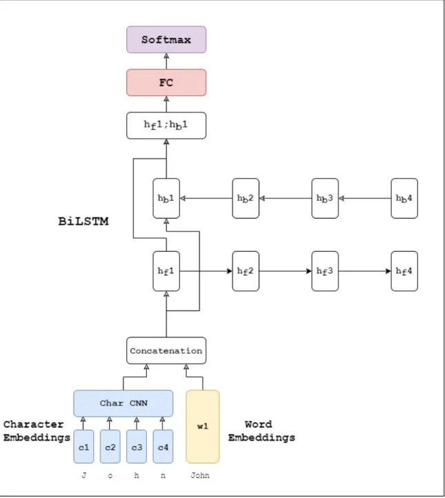
Figure 5.8 A GloVe+CNN+BiLSTM base model example. The arrow indicates the direction of the output from previous layer passing as input to the next layer. . . 27

Figure 5.9 The prediction procedure of combining models trained on separate tasks . . . 29

(10)

Chapter 1

Introduction

In this thesis, we propose a multi-task framework designated for Lexicalized Tree Adjoining Grammar (LTAG) supertagging neural models, which greatly improves the tagging accuracy of the model being applied without additional resources of labeled data. We design and select 5 auxiliary tagging tasks based on the experiment results, and the tag label of each task is derived by deconstructing the tree-like supertag structure, and every task captures certain syntax characteristics of supertags. We apply our multi-task framework into various neural models, and experimental results show that our framework can consistently help to improve the prediction accuracy regardless of what model is applied with. We also present error analysis comparing prediction results before and after applying the framework, as it clearly indicates that our multi-task framework excels in the disambiguation of easily confused supertag pairs.

1.1

Motivations

Supertagging, first introduced by Joshi and Srinivas (1994), is a sequence prediction task which assigns each lexical item in a sentence with a rich syntax representation, in order to reduce the global parsing complexity and so be called “Almost parsing”. Many prior works (Sarkar, 2007; Kasai et al., 2018) have shown that combining a parser with su-pertagger can substantially help either statistical or neural network-based parsing methods in reducing the lexical ambiguity and improving parse efficiency. Even though there is a wider interest in researching supertagging over Combinatory Categorial Grammar (CCG; Steedman, 2000), we focus on LTAG supertagging as the LTAG supertagging is a more challenging task in having a larger set ofsupertags. Also, TAG supertagging has a well-defined tree-like structure where we can easily (every LTAG supertags is also an elementary tree) extract representing features of each supertag.

Structural features of supertags are heavily used in pre-neural statistical parsing meth-ods (Bangalore et al., 2009) and proved to be useful. Chen et al. (2006) and Chung et al. (2016) trained a feature-based classification model for TAG supertags. Neural

(11)

network-based supertagging models in TAG (Kasai et al., 2018) and CCG (Xu et al., 2015; Xu, 2016; Vaswani et al., 2016) have shown substantial improvement in performance, but the supertagging models are all quite similar as they all use a bi-directional recurrent neural network (RNN) feeding into a prediction layer and treat the supertagging task just like any other tagging tasks without using any information provided by the supertag. The use of supertag structure was explored in Friedman et al. (2017) where they adopt grammar features into a tree-structured neural model over the supertags but this model was unable to beat the state-of-the-art. Kasai et al. (2018) combines supertagging with parsing which does obtain state-of-the-art accuracy, but uses additional parse data for joint-training and still, does not exploit the rich structural information behind each supertag.

The fact that none of the prevailing neural-based supertaggers utilizes the rich tree-like structures of supertags leads us to consider how to capitalize on the innate characterics of supertags. As a neural supertagger construct a probability distribution of possible supertags, we seek a way of differentiating between possible choices predicated on structural features of these supertags themselves. Beyond that, we wish to develop a framework that can easily migrate between different grammars. Last but not least, we also explore an automatic process of extracting the key characteristics without resorting to heuristically handcrafted features.

1.2

Contributions

The contributions of this work are:

• We implement the previous state-of-the-art supertagging model (Kasai et al., 2018) and discover that the most frequently confused pairs of supertags have great similarity in structures.

We discover that the previous state-of-the-art supertagging model always confuses pairs of supertags which share similar elementary tree structure but differ in small components of the tree.

• We provide several novel ways to deconstruct supertags to create multiple alternative auxiliary tasks.

The deconstruction of supertags reveals the linguistic meanings of each supertag.

• We develop a multi-task framework that exploits the deconstructed auxiliary tasks and obtain the state-of-the-art result.

Unlike most other work in multi-task learning with neural models, we do not use differ-ent annotated datasets for each task. We use exactly the same training data set but we construct multiple tasks with alternate output labels by automatically deconstructing the supertags (the output labels in the original task). The multi-task framework is

(12)

also easily applicable to any supertagging models and expects to consistently improve the performance of any model in terms of prediction accuracy as we show in this work.

1.3

Overview

Chapter 2 of this thesis reviews the tree-adjoining grammar (TAG) and TAG supertag. In Chapter 3, we review the basics of neural networks and further explain RNN, long short-term memory (LSTM) networks, character embeddings, Glove word embeddings, and highway connections as they are used in our implementation. In Chapter 4, we introduce the deconstruction of supertags, five auxiliary tasks, and our multi-task framework. In Chapter 5, we present and discuss the result and in Chapter 6, we conclude with a discussion of future work.

(13)

Chapter 2

Related Work

Before neural network approaches, statistical models (Bangalore and Joshi, 1999) or feature-based classification models (Bangalore et al., 2009; Chung et al., 2016) were widely used for supertagging. Bangalore et al. (2009) and Chung et al. (2016) trained a feature-based classification model for TAG supertags, that extract features using lexical, part-of-speech attributes from the left and right context in a 6-word window and the lexical, ortho-graphic (e.g. capitalization, prefix, suffix, digit) and part-of-speech attributes of the word being supertagged.

Seeing the effectiveness of applying neural network methods for the sequence prediction tasks (POS tagging, chunking, semantic role labeling, etc.), researchers naturally shifted their attention and had great success in applying NN methods for supertagging as well. Lewis and Steedman (2014) first applied the feed-forward neural network (FNN) model, which was originally introduced by Collobert et al. (2011) for addressing the POS tagging, for CCG supertagging and obtained an accuracy of 91.57% on the CCGBank dataset. Later, Xu et al. (2015) employed the Elman recurrent neural network (Elman, 1990) and showed a 0.47% accuracy improvement compared to Lewis and Steedman’s NN-based model. Concurrently, Xu et al. (2016) explored bidirectional RNN models, Vaswani et al. (2016) and Lewis et al. (2016) used bidirectional LSTMs with a different training procedure, obtaining accuracies of 93.52%, 94.50% and 94.30% respectively. Then, Xu (2016) integrated the attention mechanism with LSTM and achieved an accuracy of 94.46%.

Neural network-based supertagging models in TAG (Kasai et al., 2018, 2017) and CCG (Xu et al., 2015; Lewis et al., 2016; Xu, 2016; Vaswani et al., 2016) have shown substantial improvement in performance, but the supertagging models are all quite similar as they all use a bi-directional RNN feeding into a prediction layer. Structural features of supertags are heavily used in pre-neural statistical parsing methods Bangalore et al. (2009) and proved to be useful. The use of supertag structure was explored in Friedman et al. (2017) where they adopt grammar features into a tree-structured neural model over the supertags but this model was unable to beat the state-of-the-art. Kasai et al. (2018) combines supertagging

(14)

with parsing which does provide state-of-the-art accuracy but at the expense of computa-tional complexity.

Kasai et al. (2017) adopted the Bi-LSTM into the TAG supertagging, the BiLSTM model takes both the word embedding and predicted POS tag embedding as inputs. On top of it, Kasai et al. (2018) train a BiLSTM supertagger jointly with a graph-based parser. They also add the Character CNN and Highway Connection to the BiLSTM and achieve an accuracy of 91.01% on the TAG-annotated WSJ Penn Tree Bank. This work had state-of-the-art accuracy before our paper on the Penn treebank dataset.

Friedman et al. (2017) investigated a recursive tree-based vector representation of TAG supertags, but while their model can learn useful facts about supertags, about how one can be related to another, there was no performance improvement as a result of their model on the supertagging task.

Neural methods have achieved the competitive result that outperforms statistical and feature-based classification models. However, all works presented before do not take full advantage of the complex structural information contained within each supertag. They all treat the supertagging like other tagging tasks like POS tagging so that the model leans to be consistently confused with pairs of supertag trees that have similar structures. We are looking for the approaches that utilize such information and our multitask framework is born with this purpose.

(15)

Chapter 3

TAG and Supertag

In this chapter, we first go through the definitions of Tree Adjoining Grammar (TAG) in section 3.1. Second, we introduce the adjoining and substitution operations in section 3.2 and discuss the adjoining constraints in section 3.3. We then briefly demonstrate the derivation tree of TAG in section 3.4 and lexicalized TAG in section 3.5. Finally, we present the supertag in section 3.6.

3.1

Tree Adjoining Grammar

According to definition in Joshi and Schabes (1991), a tree adjoining grammar (TAG) consists of a quintuple (Σ, N T, I, A, S), where

(1) Σ is a finite set of terminal symbols;

(2) N T is a finite set of non-terminal symbols;

(3) S is a distinguished non-terminal symbol: S∈N T; (4) I is a finite set of finite trees, calledinitial trees;

(5) A is a finite set of finite trees, calledauxiliary trees;

An example of the initial tree and auxiliary tree is shown in Figure 3.1. An initial tree has the following characters:

• interior nodes are labeled by non-terminal symbols;

• the nodes on the frontier of initial trees are labeled by terminals or non-terminals; non-terminal symbols on the frontier of the trees inI are marked for substitution; by convention, we annotate nodes to be substituted with a down arrow (↓);

On the other hand, an auxiliary tree, which is able to represent recursive structures, is characterized by the following properties:

(16)

S

NP0 ↓ VP

V

loved

NP₁ ↓

(a) Initial Tree

VP

V

has

VP∗

(b) Auxiliary Tree

Figure 3.1: Example of initial tree and auxiliary tree.

• interior nodes are labeled by non-terminal symbols;

• the nodes on the frontier of auxiliary trees are labeled by terminal symbols or non-terminal symbols. The non-non-terminal symbol on the frontier of the trees in A are marked for substitution except for one node, called the foot node; by convention, we annotate the foot node with an asterisk (∗); the label of the foot node must be identical to the label of the root node.

For both trees, terminal nodes in this thesis will be labeled with ; In lexicalized TAG, at least one terminal symbol (the anchor) must appear at the frontier.

The union set of I and A together forms the set of elementary trees. We can build a complicated derived tree by composition of initial and auxiliary trees via two operations:

adjoining and substitution, which we will elaborate in the next sub section.

3.2

Adjoining and Substitution Operations

Adjoining operation builds a new tree from an auxiliary tree β and another tree (either initial or auxiliary tree) α. Let α be the tree to be adjoined into, α contains the non-substitution noden of which the label isX. Meanwhile, the root of the other auxiliary tree β must have the same label as X, and adjoiningβ toα at noden is performed as following steps (see illustration in Figure 3.2):

• the sub-tree of α rooted byn, noted ast is detached, leaving n inα as it is.

• the auxiliary treeβ is attached atn and its root node overlaps n.

• the sub-tree t is attached to the foot node of β with the root node identified as the the foot node ofβ.

(17)

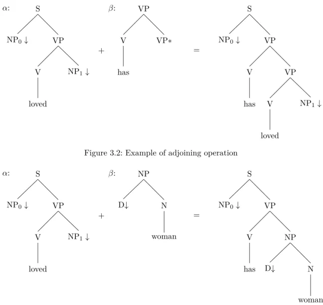
α: S NP₀↓ VP V loved NP₁ ↓ + β: VP V has VP∗ = S NP₀↓ VP V has VP V loved NP1 ↓

Figure 3.2: Example of adjoining operation

α: S NP₀↓ VP V loved NP₁ ↓ + β: NP D↓ N woman = S NP₀↓ VP V has NP D↓ N woman

Figure 3.3: Example of substitution operation

Substitution replaces a non-terminal leaf node (marked with ↓) with another tree of which the root node has the same label as the node to be replaced. Only trees derived from initial trees can substitute. An illustration of substitution is given in the Figure 3.3:

3.3

Adjoining Constraints

With the adjoining operation defined in the Section 3.2, any auxiliary tree can adjoin to a tree at certain nodenif the auxiliary tree has the same root node label asn. Such operation is done independently of the context around the node n.

A TAG can be furthered defined with the local constraints (Vijay-Shankar and Joshi, 1985). G = (I, A) is a TAG with local constraints if for each node n, in each tree t, one (and only one) of the following constraints is specified:

(18)

S

e

I: α: A: β: S(∅)

a S

b S(∅) c

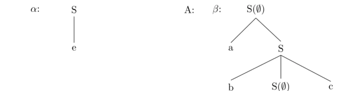
Figure 3.4: G = (I,A) that generates the language {anbncn|n >= 1}, a, b, c, e are terminal symbols.

(1) Selective Adjoining (SA): Only a subset of all auxiliary trees are specified to be ad-joinable at a certain node. SA is usually written asC.

(2) Null Adjoining (NA): No auxiliary is adjoinable at the node N. NA is usually written as∅.

(3) Obligatory Adjoining (OA): At least one auxiliary tree must be adjoined at the node n. OA is usually written as O(C) whereC is a subset of the set of all auxiliary trees adjoinable at n.

With the local constraints, TAG is able to generate languages that a context-free gram-mar (CFG) cannot generate. For example, a TAG G = (I,A) with the local constraints can express the language{anbncn|n >= 1}as in Figure 3.4. Since we specify the NA at the root node and the leaf node labeled with S, the only adjoinable node is the one in the center. This is an example of why the TAG is more powerful than CFG. However, as pointed out by Joshi (1985), it still lacks the ability to express some languages such as L= (an2|n >= 1).

3.4

Derivation Tree

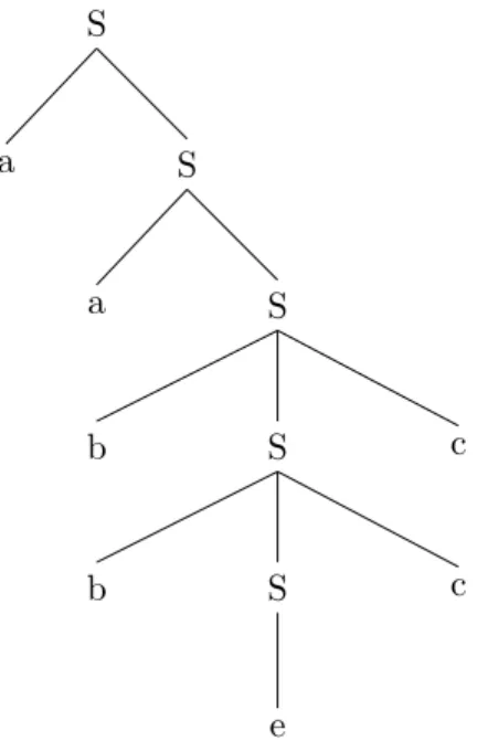
A derivation tree is an object that specifies uniquely how a derived tree was constructed (Joshi and Schabes, 1991). The derived tree does not tell us enough information about how it was constructed. The derivation tree shows how the derivation process is made. A sample derived tree is shown in Figure 3.5. It bases on the grammar defined in 3.4 and expresses the language {aabbecc}. The corresponding derivation tree is demonstrated in Figure 3.6. The dashed line represents the substitution operation and the unbroken line indicates the adjunction. The derivation tree in Figure 3.6 can be interpreted as follow: the initial treeα is substituted to the node (2,1) (the leaf S) of the parent tree β, and the auxiliary tree β is adjoined to itself at the node (1,1) (the centreS). It results in the derived tree shown in Figure 3.5.

(19)

S a S a S b S b S e c c

Figure 3.5: The derived tree using the grammar defined in Figure 3.4.

(20)

3.5

Lexicalized Tree Adjoining Grammar (LTAG)

The lexicalization of TAG is a process of finding a formalism F’ for the formalism F, so that for any finitely ambiguous grammar G in F there is a grammar G’ in F’ such that G’ is a lexicalized grammar and such that G and G’ generate the same language (Joshi and Schabes, 1991). The lexicalization procedure assigns the linguistic meanings to TAG and makes it go beyond the formalism. Each elementary structure is associated with a lexical item calledanchor (Joshi, 1985). The finite set of structures each associated with an anchor is calledlexicon. The structures of the lexicon are called elementary structures. Structures obtained from operations are called derived structures. A lexicalized structure can have more than but at least one overt lexical item that appears in it.

An important property is that lexicalized tree adjoining grammars are finitely ambigu-ous. A grammar is finitely ambiguous if there is no such sentence with a finite length that can be parsed in infinite many of ways. LTAG is finitely ambiguous is because the set of selectable structures is finite, these structures can only be combined in finitely many ways. Therefore the search space for analysis is finite and the recognition problem for LTAG is decidable.

3.6

Supertagging

Part-of-speech tagging (POS) is often used to simplify the parsing problem by providing POS tags as input. The tagging is usually local as it only accesses a limited context to infer which tag should be assigned for each token. In lexicalized Tree-Adjoining Gram-mar (LTAG), each lexical item is associated with at least one elementary tree (Joshi and Srinivas, 1994). The elementary tree is also called supertag, in order to distinguish them from the POS tags.

The supertag can be regarded as a more powerful POS tag as it contains the POS tag with the presence of the head node, whom label is exactly the POS tag. The supertag-ging task is a sequence prediction task that assigns each lexical item in a sentence with the supertag. The advantage of the supertag is that it localizes and contains much richer information than the POS tag so that given the supertags of each token in a sentence, we can quickly and effortlessly combine them together to obtain the full parse tree.

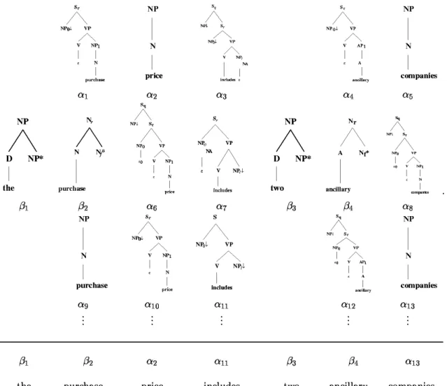
An example from Bangalore and Joshi (1999) is shown in figure 3.7. Figure 3.7 depicts the set of supertags associated with each token of the sentencethe purchase price includes two ancillary companies. The label of supertag is slightly different from the naming convention used in this thesis but the supertag structures are consistent with the rest of thesis.αn and

βn denote auxiliary tree and initial tree respectively.

In general, a TAG takes O(n6) complexity to parse a sentence of n words (Satta, 1994; Sarkar, 2007), while a CFG only takes O(n3). Motivated by the POS disambiguation

(21)

(22)

niques to eliminate the POS ambiguity prior to parsing, LTAG supertagger is used in TAG parsing to speed things up.

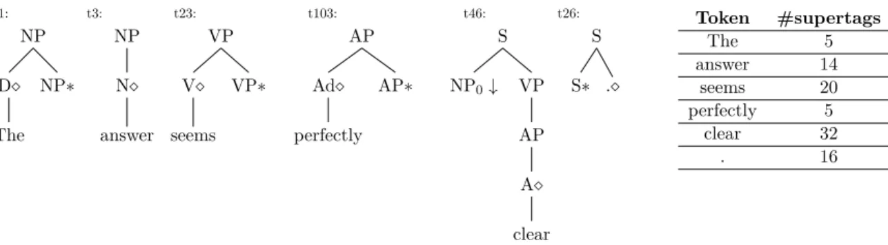
NP NP∗ D The t1: NP N answer t3: VP VP∗ V seems t23: AP AP∗ Ad perfectly t103: S VP AP A clear NP0↓ t46: S . S∗ t26: _Token _#supertags The 5 answer 14 seems 20 perfectly 5 clear 32 . 16

Figure 3.8: An example that explains the supertagging task for Tree Adjoining Grammars (TAGs). For the sentence “The answer seems perfectly clear .” the correct supertag for each word is shown above. The table on the right shows how many different supertags are possible for each word in the sentence.

On the other hand, multiple supertags can be associated with a word, thus increasing the local ambiguity, while the word always has one single unique POS tag in a sentence. An example of the supertagging task for Tree-Adjoining Grammars (TAGs) is shown in Figure. 3.8 (Zhu and Sarkar, 2019). In this example, each word in the sentence has at least 5 supertags that could potentially be associated with. The supertagger helps pick the most suitable supertag hence reducing the number of possible combinations that a parser would process.

3.7

Conclusion

In this chapter, we briefly review the basics of Tree adjoining grammars (TAG) about the adjoining and substitution operations, adjoining constraints, derivation tree and lexicalized tree adjoining grammars (LTAG). We also provide an overview of the concept of supertag and the importance of supertagging task. TAG and supertagging are foundations of this work as we extract the auxiliary tasks (Section 5.1) based on the characteristics of the elementary tree.

(23)

Chapter 4

Neural Networks Background

The concept of the neural network was brought up by McCulloch and Pitts (1943), and in the late 1940s, Hebb (1949) proposes the Hebbian theory, which is often summarized as cells fire together and wire together (Lowel and Singer, 1992). The theory suggests that the neurons are interacting with each other to fire response when receive external stimulus, create or adapt such connections according to the feedback.

Inspired by the biological neurons of the human brain, artificial neural networks (ANN) comes into being. The ANN is generally a directed, weighted graph: every node in this graph is a neuron and the edge between two nodes is analogous to the biological connections between two neurons. By taking the inputs (external stimulus) and processing it through the ANN, we are able to respond with an output (action) and further receive the feedback. The feedback allows us to update the strength of connections between every pair of neurons via back-propagation.

In this chapter, we start from reviewing the simplest neural network structure - percep-tron in 4.1, and continue on the general feed-forward neural network and go through the back-propagation, which plays a key role in the training of weights of neural networks, in 4.2; In 4.3 and 4.4, we discuss the recurrent neural network (RNN) and Long-short Term Memory (LSTM) as they are prevailing methods in sequence prediction tasks; In 4.6 and 4.7, we talk about the Glove word embedding and character CNN, which are critical components of the base model.

4.1

Perceptron

The perceptron is a supervised binary classification algorithm (Rosenblatt, 1958). A per-ceptron learns a binary classifier that takes a real-valued vector as input and generates a binary output. The binary classifier is also called threshold function formulated in Equation 4.1: f(x) =    0 if w·x+b≤p 1 otherwise (4.1)

(24)

x is the input vector, w is the weight vector and w·x is the dot product and b is the bias. Perceptrons are powerful in learning classification rules for the linear separable data. However, it cannot deal with linearly nonseparable data. The most famous example is the boolean XOR problem. The learning algorithm of the perceptron is fairly easy as a two-step method. For each training sample xi, yi, and current weightw, we update the weight by

w0 =w+r·(yi−f(w, b, xi))·xi (4.2)

w0 is the new weight and f is the function defined in Equation 4.1. The perceptron can be considered as an artificial neuron with the Heaviside step function as the activation function. The single-layer perceptron is the simplest feed-forward neural network.

4.2

Feed-forward Neural Network

An extension to the single-layer perceptron is to have multiple computational units inter-acted in a feed-forward way. The output of a neuron in one layer is the input to the neuron of the subsequent layer. In general, any directed acyclic graph may be used for a feed-forward network. Each node can be a neuron, input or output. Various activation functions might be used, and there can be relations between weights, as in convolutional neural network (CNN). The multi-layer neural network might require a variety of training techniques. Back-propagation is one of the most popular techniques. Given a structured neural network, how to efficiently optimize the parameter θ becomes a challenge to minimize the loss E(y,yˆ), whereyis the predicted value ad ˆyis the reference. Gradient descent is a first-order iterative optimization algorithm commonly used in finding the local minimum of a neural network. It can be formulated as Equation 4.3

ω=ω−γ∂E(y,yˆ)

∂ω (4.3)

where some weight ω ∈θ and γ is the learning rate. The term γδE_δω(y,yˆ) is usually referred as step size. When using gradient descent for finding the local optimal parameters, we first initialize the parameter with certain values, and pass the inputs x through the model to get the predicted value; then we calculate the step size and update the weight following Equation 4.3; repeatedly performing the last two steps until the step size is below the threshold.

Stacking more and more layers into a neural network makes the computation of the gradient complicated and time-consuming. The back-propagation technique avoids duplicate computation by calculating the gradient of weights layer by layer, and that greatly improves the efficiency of this computational process. For example, in a feed-forward network, the error term δ(k) = ∂E_∂a(₍y,_k₎yˆ), where a(k) is the output of k-th layer (after activation) can be

(25)

decomposed via applying the chain rule into the product of δ(k) = ∂E(y,yˆ) ∂a(k) = ∂E(y,yˆ) ∂a(k+ 1)∗ ∂a(k+ 1) ∂z(k+ 1) ∗ ∂z(k+ 1) ∂a(k) (4.4)

where _∂a∂E₍(_ky,₊₁₎yˆ) =δ(k+ 1). Thus, the error term can be updated layer by layer in a backward fashion. As for the weight of each layer, the gradient is

∂E(y,yˆ) ∂W(k) = ∂E(y,yˆ) ∂a(k) ∗ ∂a(k) ∂z(k) ∗ ∂z(k) ∂W(k) =δ(k+ 1)∗ ∂a(k) ∂z(k) ∗ ∂z(k) ∂W(k) (4.5)

The terms _∂z∂a(₍k_k)₎ and _∂W∂z(₍k_k)₎ can be easily derived and the error term δ(k+ 1) is already computed from last layer hence the efficiency of back-propagation.

4.3

Recurrent Neural Network

The feed-forward neural network is powerful for fixed-size input, but the nature of FNN limits its ability to process the variable-length sequences of inputs. Therecurrent neural network (RNN) was designed with the purpose of tackling this issue. An RNN usually shares the weight among time steps, and it takes the sequence input and the hidden state vector representing the context based on prior input and output. The mechanism of the hidden state allows the RNN to remember information in history, which makes it a natural fit for natural language processing (NLP) tasks. There are many variants of RNN architectures, and one of the most popular is long-short term memory (LSTM), which we now introduce it in Section 4.4.

4.4

Long-short Term Memory

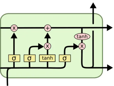
Even though RNN has the ability to handle the variant length input, RNN has a vital weak-ness in that the gradient of the early time step is prone to vanish (tend to 0) or explode (in-finite) when back-propagating. To address this issue, Long-short Term Memory (LSTM) architecture was introduced by Hochreiter and Schmidhuber (1997). A popular illustrative diagram of a LSTM unit is shown in Figure 4.1. Intuitively, a LSTM unit has an input gate, an output gate and a forget gate for controlling the flow of information, and a memory cell responsible for remembering the history. LSTM is able to partially overcome the gradient exploding or vanishing problem, however, with a long sentence input, it could still fall into

(26)

Figure 4.1: Demonstration of LSTM cell architecture

the same issue again. The mathematical equations of LSTM with a forget gate are

ft=σg(Wfxt+Ufht−1+bf) it=σg(Wixt+Uiht−1+bi) ot=σg(Woxt+Uoht−1+bo) ct=ft◦ct−1+it◦σc(Wcxt+Ucht−1+bc) ht=ot◦σh(ct) (4.6)

wheref is the forget gate, ois the output gate,iis the input gate, cis the memory cell, h is the hidden state,Wf, Wi, Wo, Wc are weights for the input vector, and Uf, Ui, Uo, Uc are

weights for the hidden state, and the index tindicates the time step.

A bidirectional LSTM is a simple but effective extension to LSTM. The idea is to not just feed the input sequence forwardly, but also backwardly hence two representation ←h−t

and −→ht at one-time step. Figure 4.1 illustrates the structure of a BiLSTM. BiLSTM has

been proven to be useful in many sequence prediction works, and we use this architecture as well in the implementation of our base model for our experiments.

4.5

Multi-task Learning

Multi-task learning (MTL) (Caruana, 1997) learns multiple heterogeneous tasks in parallel with a shared representation so that what is learned for one task can be shared for another

(27)

lobert and Weston, 2008; Luong et al., 2015). While some combinations may not provide any benefit in MTL (Bingel and Søgaard, 2017) and the improvements might be simply due to training on more data. However, MTL can be effective even when using large pre-trained models (Liu et al., 2019).

Unlike most other work in multi-task learning with neural models, we do not use dif-ferent annotated datasets for each task. Similar to the approach to combining difdif-ferent representations for phrase structure parsing in (Vilares et al., 2019) we also construct mul-tiple tasks from exactly the same training data set. Our approach is also distinct in that we take advantage of the structure of the supertags by deconstructing the tree structure implicit in each supertag.

4.6

Word Embedding and Glove

Words are easily understandable by human beings but impossible for a computer. Word embedding refers to methods that map a word to its numerical vector representation in a lower dimension space. The invention of Word2Vec (Mikolov et al., 2013) led the trend of word embeddings. In this thesis, we use the pre-trained Global vectors for word represen-tation (GloVe; Pennington et al., 2014) in the embedding layer to our model.

GloVe can encode the semantic similarity between a pair of words in word embedding space. With GloVe, we can tell if two words share similar meanings by measuring the distance between their embedding vectors. For example, the distance between the embedding vectors of "dog" and "puppy" is much smaller than the distance between the vectors of "dog" and "basketball". In order to achieve this goal, the first step of GloVe is to build a co-occurrence matrix X with the corpus, where Xij is the number of times that a word i

and its context word j co-exist in a context window. A decreasing weighting function is applied so that two words that are far away from each other contribute toXless than those are close. The estimation of the relationship between co-occurrence matrix X and word embedding vector is formulated as Equation 4.7

W_iTW˜j +bi+ ˜bj = log(Xij) (4.7)

whereWi and bi are the word vector and bias for word i, ˜Wj and ˜bj are the contextword

vector and bias for wordj.

A weighted mean square loss function is used for training as Equation 4.8

J =

V X

i,j=1

f(Xij)(WiTW˜j+bi+ ˜bj −log(Xij))2 (4.8)

The goal is to reduce the difference between the co-occurrence times of two words and the dot product of their word vectors.f is a non-decreasing weighting function that weighs

(28)

more on the frequent pairs but prevents them from being overweighed compared to rare pairs by setting a threshold.

4.7

Character Embedding and Character CNN

Similar to word embedding, characters can be projected into a numerical vector as well. Character embeddings are usually combined together with word embedding as inputs, pro-viding additional lexical features. The motivation behind the character embedding is that characters in a word capture morphological information and provide clues to the grammat-ical properties such as part-of-speech. For example, a word ending with "ly" is very likely to be an adverb in English. While word embedding extracts semantic relationships between words, character embedding aims at finding the morphological evidence (Ling et al., 2015). After converting every character of a word into a character embedding vector, we obtain a sequence of character embedding vectors. Generally, we need to encode the sequence of character embedding vectors into a single fixed-length vector and concatenate it with the word embedding as a final input vector to the neural network. Since it is a variant length sequence encoding problem, encoding with LSTM is often used (Lample et al., 2016).

Another alternative method is to use the Character Convolutional Neural Network (CNN). For a word consisting ofLcharacters and the sequence of character embeddingsc1, c2, ..., cL,

the convolutional layer applies a matrix-vector operation to each window of size k for the character embedding sequence. The concatenation zi of the character embeddings around

theith character of window size ofkis denoted as:

zi = (ci−(k−1)/2, ..., ci−(k+1)/2) (4.9)

The convolutional layer then computes thej-th element of r, the final character-level em-bedding of the word, as follows:

rj = max

1<i<L[W zi+b]j (4.10)

The character embedding matrix, and matricesW andbare parameters to be learned. After obtaining the vectorr, we then concatenate r with the word embedding vector w as input to our models.

4.8

Conclusion

In this chapter, we review the basics of neural networks including perceptron, FNN, RNN, LSTM. We compare other multi-task learning methods with our multi-task framework and also introduce key components such as pre-trained word embeddings, character embeddings

(29)

and character CNN of our base model. The detail of our multi-task framework is explained in the next chapter.

(30)

Chapter 5

Deconstructing Supertags

As discussed in Chapter 2, we hope to utilize the structural information of supertags to assist in the prediction of supertags. We train the previous state-of-the-art supertagging model and analyze the errors made by that model. An interesting finding is that the predicted supertag is often similar to the gold supertag but has small differences in terms of some structural features. We examine the most frequently confused pairs and abstract five key features of the supertag structure that the confused pairs are different at. We define the label set of each feature that we found and we formalize them as five auxiliary tasks: HEAD, ROOT, TYPE, SKETCH, and SPINE. We give a comprehensive introduction to these tasks in Section 5.1.

Another observation we made is that top-3 softmax probabilities given by the single supertagging model are fairly close. If we manage to enhance the probability of supertag prediction by taking account of the auxiliary task prediction results, we can choose the one with the highest ensembled probability as our new prediction.

Our multi-task framework is two-fold: during the training stage, we train the base model on each auxiliary task as well as the supertagging task independently; at inference time, we ensemble the prediction probability for the supertag and each of auxiliary labels. Unlike other popular ensemble methods, our multi-task framework is based on the features of the output, rather than the input.

5.1

Auxiliary Task

5.1.1 Head

The head node of a supertag tree is the leaf node that is anchored to the associated token. Recall that the supertag is also called the super part of speech tag. The label at the HEAD node is equivalent to the part-of-speech (POS) tag of this lexical item. This property explains the relationship between the supertag and the POS tag: knowing the supertag automatically gives us the POS tag of the word. Even though a word has a unique POS, there might be

(31)

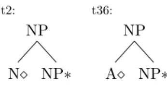
NP NP∗ N t2: NP NP∗ A t36:

Figure 5.1: The grammar of supertag t2 and t36

Thus, the prediction of the HEAD node label is basically the same as solving the task of POS tagging.

Many supertags have almost identical structures but only differ in the head node. For example, the baseline supertagger wrongly predicts the supertag t36 as t2 in the dev set 194 times. The structure of t2 and t36 can be found in Figure 5.1.

t2 is headed by a noun head N and t36 is headed by an adjective A. The overall structure (or SKETCH) and the label of other nodes are all the same. Understandably, the model is confused between these two supertags since they are often used in scenarios that even a human could not immediately distinguish. An instance of sentence that contains supertag t2 and t36 is: “More than a few CEOs say the red-carpet treatment tempts them to return to a heartland city for future meetings.” and the sequence of supertag matches to this sentence is t73 t4 t1 t36 t3 t28 t1 t36 t3 t28 t29 t31 t81 t44 t1 t2 t3 t13 t36 t3 t26. The words “few”, “red-carpet” and “future” are assigned with t36, while the word "heartland" is assigned with t2. The phrases in which those words reside are “few CEOs”, “red-carpet treatment”, “heartland city” and “future world”. Without the context, the word “future” can be a noun or an adjective. Here the word “future” is labeled as an adjective because of the lack of a determiner, but we can still tell from this instance how similar t2 and t36 are being assigned.

Ideally, if we can have an omniscient HEAD (POS) tagger, of which the prediction accuracy is 100%, we can immediately correct these misclassified supertags. Till now, a trivial BiLSTM HEAD (POS) tagger can easily achieve an accuracy of 97% for the Penn Treebank dataset. The base model we used in this thesis can achieve similar accuracy. We define a function HEAD (t) to get the head node (marked by a diamond) of supertag t. There are 29 distinct HEAD labels extracted from the supertag set.

5.1.2 Root

The ROOT task is another task that predicts the label of a certain node of the supertag tree. The root bridges multiple subtrees of the supertag tree and implies the dependency relationship between these subtrees, particularly for the auxiliary tree. An auxiliary tree can be only adjoined to a non-substitution node with the same label as its root. In other words, the label of the root node is also the label of the foot node.

(32)

NP N t3: FRAG NP N t207:

Figure 5.2: The grammar of supertag t3 and t207. Both of them are initial trees.

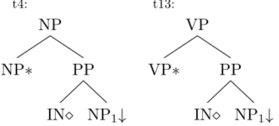
NP PP NP1↓ IN NP∗ t4: VP PP NP1↓ IN VP∗ t13:

Figure 5.3: The grammar of supertag t4 and t13. Both of them are auxiliary trees.

t3 and t207 is a pair of initial trees that are commonly confused by the baseline model. The grammar of t3 and t207 is presented in Figure 5.2. These two share the same HEAD node label (N) and are slightly different in the overall shape, but the biggest difference is the root node label, where t3 has NP as root and t207 has FRAG.

In the case of auxiliary trees, a great example is t4 and t13. There are 78 t4 being predicted as t13, and 72 t13 being predicted as t4 by the baseline model. The grammar of supertag t4 and t13 can be found in Figure 5.3.

t4 modifies an NP node while t13 modifies a VP node. They have overall same shape (SKETCH), head node label (the node with diamond) and substitution node label (the node with down arrow). This is a case of preposition attachment ambiguity.

We define a function ROOT (t) to get the root node of supertagt. We extract 48 distinct ROOT labels from the supertag set.

5.1.3 Type

Follow the thinking above, we observe another pattern that the baseline model frequently mixes up, which is the tree TYPE of supertag. According to the definition in Section 3.1, an elementary tree can be classified into two types: initial tree and auxiliary tree depending on the recursive structure.

Consider the type of trees t2 and t3. A comparison between the grammar of t2 and t3 can be found in Figure 5.4. t2 is an initial tree while t3 is an auxiliary tree, that results in a slight difference in the overall shapes. Other than that, they have the same root node (NP)

(33)

NP N t3: NP NP∗ N t2:

Figure 5.4: The grammar of supertag t3 and t2. t2 is an initial tree and t3 is an auxiliary tree. NP NP∗ " t5: NP " NP∗ t6:

Figure 5.5: The grammar of supertag t5 and t6. t5 is adjoined from the right side since the foot node is in the right sub-tree to the root while t6 is the opposite.

and head node (N). There are 44 times where the baseline supertagger predicts t2 as t3 and 6 times where the supertagger predicts t3 as t2.

We experiment with our multi-task framework with the task of predicting if a supertag is an initial tree or an auxiliary tree. However, the effect of such a task is not obvious. We further define the TYPE task by considering where the auxiliary tree is adjoined, depending on where the foot node of an auxiliary tree locates at. An example of a left-auxiliary tree and the right-auxiliary tree is shown in Figure 5.5. The foot node (NP with a start notation) of t5 resides in the right sub-tree to the root, so we consider it as aright auxiliarytree. t6 is the opposite, and we label it as a left auxiliarytree. By doing so, we end up with three labels of TYPE task: I (initial tree), L (left auxiliary tree) and R (right auxiliary tree).

Unfortunately, our research shows that there still is no improvement after this extension. A further enhancement to this task is to take account of the root node label collectively with the left or right adjoining direction. We generate the label in the form ofT reeT ype+ RootN odeLabel. TheT reeT ypeincludes three types: initial left and right. We reuse the set of root node labels from Section 5.1.2. For example, the type of t5 isRight+N P and the type of t6 isLef t+N P, shown in Figure 5.5. The type of t3 in Figure 5.4 isInitial+N P. The type of t13 in Figure 5.3 is Lef t+V P. We define a function TYPE (t) to obtain the type of each supertag. There are 67 distinct types.

5.1.4 Sketch

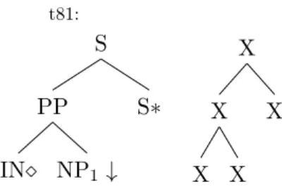
In many cases, the overall shape of the supertag is useful for disambiguation, disregarding the node labels. Intuitively, the tree structure should tell us the most information about the uniqueness of each supertag tree. The following example keeps the tree structure of the supertag but removes the node labels:

(34)

S S∗ PP NP₁ ↓ IN t81: X X X X X

Figure 5.6: The grammar of supertag t81 and its SKETCH.

S S∗ PP NP₁ ↓ IN S PP IN

Figure 5.7: The grammar of supertag t132 and its SPINE.

Two supertags have the same SKETCH as long as they have the same shape, regardless of the node label, the node attribute and tree types. For example, t5 and t6 in Figure 5.5 are considered to have the same SKETCH while t3 and t207 are not. We define a function SKETCH (t) that returns the sketch. There are 602 distinct supertag sketches.

5.1.5 Spine

The spine of a supertag is the path from the root node to the head node (marked by). The following example (Figure 5.7) keeps only the path from the root to the head and produces a spine supertag. Unlike the formation of SKETCH, we take the node label along the path into account but we still do not care about nodes that are not in the path. For example, the path of t132 from the root (S) to head (IN) is S - PP - IN. After serialization, the order of each node is important. If a supertag has the path S - IN - PP, then their SPINEs are considered as different. We use a function SPINE (t) to return the spine of supertag t. As expected, the number of distinct supertag spines is large, and there are 1372 different ones. Even though the number of SPINEs is almost as large as supertags, the SPINE task is slightly easier than the supertagging task itself.

The SPINE connects the root node and the head node, explicitly expressing the depen-dency relationship between the anchored word and its surroundings. Another nice property of the supertag’s tree nature is that the path from the root to a certain leaf is unique for one tree. It means that each supertag only corresponds to one SPINE label, allowing us to produce the ground truth label for this task.

(35)

5.2

Base Model

The basic structure of the tagging model used in our multi-task framework is called the base model. The base model is a general tagging model that satisfies two conditions:

• it takes an sequence of tokens as inputs.

• it outputs a sequence of predicted tags.

Theoretically, our multi-task framework can be applied to any sequence prediction model that satisfies the two conditions and the base model should expect to gain performance improvement. The base model is not limited to only neural network models but includes non-neural models as well. In this thesis, we experiment with different Bi-LSTM based models, and a base model example is shown in Figure 5.8.

5.3

Multi-task Framework

Unlike many other works in multi-task learning with neural models, the output labels of each auxiliary task are not from additional sources. We can construct the alternate label set of each auxiliary task through the definition in Section 5.1. Given a supertag and its gram-mar, we can deconstruct the supertag and know its corresponding ROOT, HEAD, TYPE, SKETCH, and SPINE label. These auxiliary tasks are easier in terms of the prediction accuracy than the supertagging task, and these new output labels are linguistically related to the original supertag.

A common criticism of a fair comparison between the multi-task and single-task learn-ing is that the multi-task settlearn-ing simply uses more labeled data instances (typically with different data sources). In our case, because we re-use the same training set for multi-task learning, we have made sure our experimental settings exactly match the previous best state-of-the-art method for supertagging (Kasai et al., 2018) and we use the same pre-trained word embeddings to ensure a fair comparison.

Since we have designed five auxiliary tasks, we train six different neural sequence predic-tion modelsindependently on the supertagging task, root node prediction (ROOT), head node prediction (HEAD), tree type prediction (TYPE), tree sketch prediction (SKETCH) and tree spine prediction (SPINE) tasks. For each task, we use the state-of-the-art baseline supertagging model as defined in Section 6.2.1. The only change is that the output size for the softmax is changed to reflect the number of output labels in each task. We obtain much higher accuracy for each of the tasks compared to the supertagging task. For example, on the dev set we obtain the following accuracies: ROOT = 97.04%, HEAD = 93.37%, TYPE = 93.14%, SKETCH = 93.74% and SPINE = 91.00%.

When doing the prediction, we combine the multiple tasks to create a decoder for the supertagging task. We run each best-trained model on every task and obtain a probability

(36)

Figure 5.8: A GloVe+CNN+BiLSTM base model example. The arrow indicates the direction of the output from previous layer passing as input to the next layer.

(37)

distribution over the label set of each task. We first run the baseline supertagger to obtain the distribution PSTAG and using this distribution we select the top-K output supertags

for each word in each sentence. We test with different values of K and we show that even K=3 gives 97% accuracy for the supertagging task. We also compute the output softmax distributions for each auxiliary task, PHEAD, PROOT, PTYPE, PSKETCH, PSPINE. Each of

these probabilities is defined as a sequence prediction task over the auxiliary tasks using the functions defined in Section 5.1.

PHEAD(t) = P(HEAD(t))

PROOT(t) = P(ROOT(t))

PTYPE(t) = P(TYPE(t))

PSKETCH(t) = P(SKETCH(t))

PSPINE(t) = P(SPINE(t))

Now we not only obtain the probability of each supertag but also know the probability of the supertag’s corresponding auxiliary task label. Instead of choosing the supertag with maximum softmax probability from the supertagging model, we can combine the probabil-ities from the different tasks. An intuitive but effective way of ensemble the probability is shown as follows:

t∗_i =arg max_t_i∈Sα1PSTAG(ti) +α2PHEAD(ti)

+α3PROOT(ti) +α4PTYPE(ti)

+α5PSKETCH(ti) +α6PSPINE(ti)

(5.1)

S is the top-K set of supertags for each word in the input sequence. The hyperparame-tersαj can be tuned. However we found in our experiments that the results were not very

sensitive to the values, and the uniform distribution over all the tasks performed the best. The model and decoding step for our multi-task model is shown in Fig. 5.9. The example il-lustrates the supertag prediction process of the input “John”. The modules named “BiLSTM for STAG” are the best-trained model for each auxiliary task. We first run the supertagging model to obtain a distribution over the supertag set. Then we look at the top-K prediction given by the supertagging model. If we choose t2, according to its grammar, we know the associated TYPE label of t2 is Left + NP, ROOT label of t2 is NN, HEAD label of t2 is NP, SKETCH label of t2 is SK4 and SPINE label of t2 is SP2. Also, we run the models and get probability distributions for each auxiliary task. We check the PHEAD(t2)

by looking at the probability of P(N P) = 0.12 and similarly for other tasks. For t2, the “probability” after ensemble equals 0.65 + 0.42 + 0.34 + 0.12 + 0.12 + 0.21 = 1.86. We do the same computation for all top-K supertags, and pick the one with the largest ensembled probability as our final prediction.

(38)

(39)

5.4

Conclusion

In this chapter, we discuss the auxiliary tasks as part of the deconstruction process. We describe the structure of the base model and introduce our multi-task framework. In the next chapter, we describe the experiment setup and results and also analyze the errors before and after applying our multi-task framework.

(40)

Chapter 6

Experimental Results and Analysis

In this chapter, we introduce the dataset that we used for the experiment. We describe the detailed structure and hyper-parameters for the base model, and we describe the training details for getting the state-of-the-art result. We also provide the settings of our multi-task framework. Additionally, we examine the contribution of each auxiliary multi-task of the multitask framework and compare the prediction results with and without applying our multitask framework.

6.1

Dataset

The set of supertags used in this thesis is from Bangalore et al. (2009), which they extracted from the Penn Treebank (Marcus et al., 1993) following the approach of Chen and Shanker (2001). The Penn Treebank is one of the most popular parsed and annotated text corpus, that includes one million words of 1989 Wall Street Journal material. Their extraction procedure results in a supertag set of 4,727 supertags (you can find the grammar file at https://mica.lis-lab.fr/d6.clean2.f.str). For a fair comparison, we use the same settings as in the previous work, which uses Sections 01-22 as the training set, Section 00 as the dev set, and Section 23 as the test set. The training, dev, and test sets comprise 39832, 1921, and 2415 sentences; 950028, 46451, 56683 tokens, respectively.

We perform our auxiliary label extraction based on the supertag set and grammar mentioned above. We extract 69 auxiliary tree TYPEs, 40 distinct types of ROOT node and 30 different types of the HEAD node, 602 tree SKETCHes, and 1372 tree SPINEs.

6.2

Experiment Setup

6.2.1 Baseline Supertagging Model

For our baseline supertagging model, we use the state-of-the-art model that currently has the highest accuracy on the Penn treebank dataset (Kasai et al., 2018). Kasai et al. (2018) integrates a character CNN for modeling morphological features and adds highway

(41)

connec-tions to alleviate the gradient vanishing problems for a deeper LSTM model. The output layer was a standard multi-layer perceptron that had a softmax output over the set of su-pertags. In addition, Kasai et al. (2018) combines supertagging with graph-based parsing and shows the improvement compared to the single supertagging model.

The main metric that we examine in this thesis is the supertagging accuracy. We com-pare the prediction accuracy before and after the baseline model applies our multi-task framework. The baseline model (Kasai et al., 2018) is jointly trained with a graph-based parsing model and has the current highest accuracy on the Penn treebank (90.81%). Three main components stand out in the baseline model: the input layer, the bidirectional LSTM component, and the output layer which computes a softmax over the set of supertags. The input to the model is a sequence of words and the output is a sequence of supertags, one per word, which makes it a standard tagging aka sequence prediction task.

Input Layer

The input is a sentence and every word in the sentence is converted to a word embedding vector by the word embedding layer. Following Kasai et al. (2018), we use two components in the word embedding:

• a 30-dimensional character level embedding vector computed using a char-CNN which captures the morphological information (Ling et al., 2015; Lample et al., 2016; Kasai et al., 2018). Each character is encoded as a 30-dimensional vector, and then we apply 30 convolutional filters with a window size of 5. This produces a 30-dimensional character embedding. The character embedding is randomly initialized.

• a word embedding initialized using GloVe (Pennington et al., 2014), of which dimen-sions are 100/200/300. If the word does not appear in GloVe, we initialized the word embedding with a random vector.

In the beginning and ending position of each sentence, a start of sentence token and an end of sentence token is added, but they are not included in the computation of loss and accuracy.

Unlike Kasai et al. (2018), we do not use predicted part of speech (POS) tags as part of the input sequence. We notice that the improvement was negligible in contrast to the overhead of training and running the POS prediction.

BiLSTM Layer

The core of this base model is a bidirectional recurrent neural network, in particular a Long Short-Term Memory neural network Graves and Schmidhuber (2005). For the hyperparam-eters, we use the settings in Kasai et al. (2018) in order to ensure a fair comparison.

(42)

Unlike Kasai et al. (2018) we do not use highway connections in our model. We did experiment with the addition of highway connections, but no improvement in accuracy over the BiLSTM-only model is observed. We decide to take out this structure.

The bidirectional representation has a dimension of 1024, as it is a combination of the representation from both directions having 512 units each. Dropout layers (Gal and Ghahramani, 2016; Srivastava et al., 2014) are inserted between the input and BiLSTM layer, between BiLSTM layers, and between recurrent time steps. The dropout rate used was 0.5. We experiment with the number of BiLSTM layers ranging from 2 to 3. In Kasai et al. (2018), they demonstrate the effect of having more than 3 layers and explain the reasons why more than 3 layers do not bring any additional benefits.

Output Layer

We concatenate hidden vectors from both directions of the last layer of the BiLSTM and pass it into a multilayer perceptron (MLP). In practice, a single layer perceptron performs just as well in this task. The number of input neurons of the single-layer perceptron equals 1024 (2×512) and the output vector size equals the number of labels for each specific task: 4727 for the main supertagging task.

Training

We train different base models independently on the supertagging, root node prediction (ROOT), head node prediction (HEAD), tree type prediction (TYPE), tree sketch predic-tion (SKETCH) and tree spine predicpredic-tion (SPINE) tasks. The base model we used is defined in Section 6.2.1. The only difference among the base models is the output size for softmax, which is changed to reflect the number of labels for each task. The prediction accuracies on auxiliary tasks using the base model are higher than the supertagging accuracy. For example, on the dev set we obtain the following accuracies: ROOT = 93.37%, HEAD = 97.04%, TYPE = 93.14%, SKETCH = 93.74% and SPINE = 91.00%.

The training also includes training the word embeddings (which is initialized using a pre-trained embedding) and the character embeddings for the character-level CNNs. The optimization goal is the negative log-likelihood of the predicted sequences of output labels. The negative log-likelihood minimizes the sum of predicted log-probabilities for the ground-truth label of each token in a sentence:

N LL(y) =− X

1≤t≤n

logP rt(yt) (6.1)

where the n is the number of tokens in a sentence, and P rt is the predicted probability

distribution over possible labels oft-th token, and ytis the ground label of t-th token.

(43)

Model Multi-task Dev Test BiLSTM3+HW+CNN+POS+GloVe100 (Kasai et al., 2018) - 90.45 90.81

BiLSTM2+GloVe100 No 89.11 90.26 Yes 89.67 90.62 BiLSTM2+CNN+GloVe100 No 89.45 90.15 Yes 90.12 90.80 BiLSTM3+GloVe100 No 89.41 90.42 Yes 90.02 90.93 BiLSTM3+CNN+GloVe100 No 89.83 90.73 Yes 90.41 91.26 BiLSTM3+CNN+GloVe200 No 89.94 90.73 Yes 90.55 91.37 BiLSTM3+CNN+GloVe300 No 89.91 90.74 Yes 90.45 91.31 Shared BiLSTM layer (BiLSTM3+CNN+Glove200) No 90.11 90.83 Yes 90.11 90.83

Table 6.1: Supertagging task results. The prediction accuracies are reported under the dev and test columns. The number following BiLSTM represents the number of BiLSTM layers; CNN refers to the word embedding model using character-level CNN; the number imme-diately after GloVe represents the dimension of the word embedding. All the differences in accuracy are significant before and after applying our multi-task framework. We trained the model that achieves the best accuracy (BiLSTM3+CNN+GloVe200) 5 times, the average accuracy is 91.32% and the variance is 0.0012. HW in Kasai et al. (2018) refers to highway connections, and POS refers to the use of predicted part-of-speech tags as inputs. HW and POS are not used in our model.

model is evaluated on the dev set, if the accuracy on dev set has not been improved for five consecutive epochs, training stops. The maximum number of epochs is 70. After obtaining the best model trained with`= 0.001, we further fine-tune the best model using`= 0.0001 for at most 10 more epochs. By conducting this step, we have seen 0.1% to 0.2% accuracy improvement varying from task to task.

After obtaining the best-trained model on each of the multiple tasks we combine the multiple tasks to create a decoder for the supertagging task.

6.3

Results

For our experiments, we implemented all of the models we discussed above in PyTorch (Paszke et al., 2017). We have various hyperparameters and Table 6.1 shows the results obtained from the different model configurations which were described in Section 6.2.1. Following the parameter setups in the previous work (Kasai et al., 2018), we experiment with pre-trained GloVe word embeddings of three different sizes: 100, 200 and 300. We obtain a new state-of-the-art result of 91.39% which is significantly better than the 90.81% result

(44)

Top-K Dev Test Top-1 89.94 90.73 Top-2 90.50 91.33 Top-3 90.55 91.37 Top-5 90.58 91.38 Top-10 90.58 91.39 Top-20 90.58 91.39

Table 6.2: Change in accuracy as K is increased when choosing Top-K supertags for rescor-ing. The model used is BiLSTM+CNN+GloVe200.

which combines supertagging with the parsing task and so is using more labeled training information used by our supertagger models. With our multi-task approach, we observe the significant improvements compared to a single supertagging base model between 0.4% to 0.65%.

6.3.1 Top-K Choice

The set of Top-K supertags from the baseline supertagging model is another factor that will affect the result. From our experiment, we discover that about 97% gold supertags are in the Top-3 predictions that a baseline supertagger makes. Table 6.2 that increasing K helps up to a point. After K=10 there is no further improvement. Increasing the size of candidate set further on that is pointless as the fact that over 99.5% gold supertags are within the Top-10 predictions.

6.3.2 Task Contribution

Table 6.3 shows the result of task ablation for each task. We experiment with various combinations of auxiliary tasks that lead to different accuracy results, but we can see that adding a new task always improves the results. The best result is obtained by using all five auxiliary tasks.

For each single task contribution, the HEAD and ROOT tasks contribute the least as expected, as they only predict the label of a certain node in the supertag tree. Particularly, the HEAD task is equivalent to the Part-of-speech tagging, and the improvement received by ensembling the HEAD task is consistent with the performance gain that has been seen in other people’s work for the supertagging task.

The TYPE, SKETCH and SPINE tasks encode richer structural information and there-fore are expected to play a better job in differentiating similar supertags. Our experimental results have verified our hypothesis as integrating each of these tasks improve the supertag-ging result more than the HEAD and ROOT task.

(45)

Multi-task setting Dev Test None 89.94 90.73 HEAD 90.00 90.79 ROOT 90.06 90.91 TYPE 90.15 91.07 SKETCH 90.25 90.99 SPINE 90.22 91.08 HEAD+ROOT 90.15 90.94 TYPE+HEAD+ROOT 90.27 91.10 TYPE+HEAD+ROOT+SKETCH 90.48 91.27 TYPE+HEAD+ROOT+SKETCH+SPINE 90.55 91.37

Table 6.3: Result of different multi-task combinations. The base model is BiL-STM+CNN+GloVe200.

and test set, the results are 90.35% and 91.13% respectively. Losing the supertagger, the prediction accuracy is still higher than a single supertagging model due to the high relevance between the auxiliary tasks and the supertagging task. The supertagging task itself can be considered as a strong auxiliary task that helps boost the performance of the multi-task framework.

6.3.3 Significance Test

We compute a significance score on the accuracy of our best model BiLSTM3 + CNN + GloVe200 with and without multi-task learning. On the dev set, using McNemar’s signifi-cance test we find that the multi-task model is significantly better than the baseline model with a p-value of 0.0062; on the test set, the p-value is 0.0064.

We evaluate