Fault-tolerant relay deployment for k node-disjoint paths in wireless sensor networks

UCC Library and UCC researchers have made this item openly available.

Please

let us know

how this has helped you. Thanks!

Title Fault-tolerant relay deployment for k node-disjoint paths in wireless sensor networks

Author(s) Sitanayah, Lanny; Brown, Kenneth N.; Sreenan, Cormac J. Publication date 2011-10

Original citation Sitanayah, L., Brown, K. N. and Sreenan, C. J. (2011) 'Fault-tolerant relay deployment for k node-disjoint paths in wireless sensor networks', 2011 IFIP Wireless Days (WD), Niagara Falls, ON, Canada, 10-12 October, (6 pp). doi: 10.1109/WD.2011.6098176

Type of publication Conference item Link to publisher's

version http://dx.doi.org/10.1109/WD.2011.6098176Access to the full text of the published version may require a subscription.

Rights © 2011 IEEE. Personal use of this material is permitted. Permission from IEEE must be obtained for all other uses, in any current or future media, including reprinting/republishing this material for advertising or promotional purposes, creating new collective works, for resale or redistribution to servers or lists, or reuse of any copyrighted component of this work in other works.

Item downloaded

from http://hdl.handle.net/10468/8964

Downloaded on 2020-06-06T00:47:46Z

Fault-Tolerant Relay Deployment for

k

Node-Disjoint Paths in Wireless Sensor Networks

Lanny Sitanayah

Mobile & Internet Systems Laboratory Department of Computer Science

University College Cork, Ireland Email: [email protected]

Kenneth N. Brown

Department of Computer Science University College Cork, Ireland

Email: [email protected]

Cormac J. Sreenan

Mobile & Internet Systems Laboratory Department of Computer Science

University College Cork, Ireland Email: [email protected]

Abstract—Ensuring that wireless sensor networks (WSNs) are robust to failures requires that the physical network topology will offer alternative routes to the sinks. This requires sensor network deployments to be planned with an objective of ensuring some measure of robustness in the topology, so that when failures occur that routing protocols can continue to offer reliable delivery. Our contribution is a solution that enables fault-tolerant WSN deployment planning by judicious use of a minimum number of additional relay nodes. A WSN is robust if at least one route to a sink is available for each remaining sensor node after the failure of up to k−1 nodes. In this paper, we define the problem for increasing WSN reliability by deploying a number of additional relay nodes to ensure that each sensor node in the initial design hasknode-disjoint paths to the sinks. We present GRASP-ARP, a centralised offline algorithm to be run during the initial topology design to solve this problem. We have implemented this algorithm and demonstrated in simulation that it improves the efficiency of relay node placement for k node-disjoint paths compared to the most closely related published algorithms.

Index Terms—wireless sensor networks; network deployment planning; relay placement; node-disjoint paths.

I. INTRODUCTION

In wireless sensor networks (WSNs), sensor nodes transmit their data wirelessly over a multi-hop network to sink nodes, where data is either processed or transmitted on through a high-speed connection. These networks are subject to failures: the wireless devices are often unreliable, they have limited battery life, transmissions may be blocked by changes in the environment, and the devices may be damaged, e.g. by weather, wildlife or human intervention. For dealing with failures, techniques for reliable routing in WSNs have been proposed and are well-understood, but to be effective these depend on a physical network topology that ensures alternative routes to the sink are available. This requires sensor network deployment to be planned with an objective of ensuring some measure of robustness in the topology, so when failures occur that routing protocols can continue to offer reliable delivery. Our contribution is a solution that enables fault-tolerant WSN deployment planning by judicious use of additional relays.

One key objective in the topology design of a WSN is to ensure some measure of robustness. In particular, one standard criterion is to ensure routes to the sink are available for all

remaining sensor nodes after the failure of up tok−1 nodes. This can be achieved by ensuring that every node in the initial design has k node-disjoint paths to the sinks: i.e. at least k paths that share no intermediate nodes. Node-disjoint paths are required to provide multi-path routing capability for some protocols [1]. Since there are sometimes data latency require-ments, there may be a limit to the path length from sensor to sink. To ensure that the sensors have sufficient paths, it may be necessary to add a number of additional relays, which do not sense, but only forward data from other nodes. Installing additional relays comes at a cost that includes not just the hardware purchase but more significantly the installation and ongoing maintenance, thus motivating solutions that minimise the number of additional relays.

The problem we address in this paper is that of finding a minimal set of relays which ensuresknode-disjoint paths for each sensor. We define the single-tiered, constrained partial fault-tolerant relay placement problem for k node-disjoint paths with length constraints for WSNs with data sinks, which we call the additional relay problem (ARP). We make no assumptions on the geographical or physical properties of the area in which the WSN is to be deployed, but we assume a limited set of possible locations for the relays, and a fully-specified connectivity graph. We propose GRASP-ARP, a local search algorithm based on GRASP [2], to be run as a centralised offline algorithm during the initial topology design, i.e. prior to network deployment and operation. Our algorithm requires repeated counting of the number of node-disjoint paths for each node, for which we use a dynamic program-ming procedure. We compare GRASP-ARP against the closest approach from the literature, and we demonstrate empirically that it finds solutions requiring 25% fewer additional relays for small values ofk. We also show that it scales better, finding solutions in reasonable time for problems with hundreds of nodes. This represents a quantifiable improvement, making it possible to compute cost-effective WSN designs that offer an assured level of reliable delivery.

The rest of the paper is organised as follows. We survey the related work in Section II, present the additional relay problem and GRASP-ARP in Section III and IV, respectively. Sec-tion V presents simulaSec-tion results and SecSec-tion VI concludes.

TABLE I

EXISTING RELAY PLACEMENT ALGORITHMS

Algorithms k Routing Deployment Fault-Locations Tolerance

Haoet al.[3] 2 2-tiered constrained partial Bredinet al.[4] ≥1 1-tiered unconstrained full Puet al.[5] ≥1 1-tiered unconstrained partial Kashyapet al.[6] ≥2 2-tiered un/constrained partial Hanet al.[7] ≥1 1-tiered unconstrained full/partial Zhanget al.[8] 2 1/2-tiered unconstrained partial Misraet al.[9] 1, 2 1-tiered constrained partial

II. BACKGROUND ANDRELATEDWORK

A WSN can be modeled as a graph G= (V, E), where V is a set of nodes andE is a set of edges. Each edge connects two nodes that are within transmission range of each other1, and the two nodes are said to be adjacent. A pathof length t between two nodes v and w is a sequence of nodes v=

v0, v1, . . . , vt=w, such thatvi andvi+1 are adjacent for each

i. A path from a node v to a set of nodes W is simply a path from v to any nodew∈W. Two nodes areconnectedif there is a path between them. A graph is connected if every pair of nodes is connected. A cutsetis a set C⊂V such that

(V−C, E↓V−C)is disconnected (whereE↓X means a set of

edges restricted to those that connect nodes inX). A graph is k-connectedif it has no cutset of size less thank. Two paths P andQfromvtowarenode-disjointif they have no nodes in common except forv andw.

The problem of placing relay nodes for increased reliability has long been acknowledged as a significant problem, and we summarise the existing algorithms for WSNs in Table I. In single-tiered networks, all nodes may forward packets from other nodes, while intwo-tierednetworks, sensor nodes trans-mit their own data directly to a cluster head. In connectivity problems, the aim is to ensure the network is connected (or k= 1), while insurvivable problems, the aim is to ensure k -connectivity for k >1. In unconstrained problems, the relay nodes can be placed anywhere, while inconstrainedproblems, they are limited to a set of candidate locations. Partial fault-tolerance requires k-connectivity between every sensor node, whilefull fault-tolerancerequiresk-connectivity between both sensor and relay nodes. We choose to focus on single-tiered networks as this is most common in the research literature and for published WSN deployments. Furthermore we assume the constrained approach for possible relay locations, which we believe is more reasonable for real-world deployments. Finally we assume partial fault-tolerance, reflecting the fact that relays are for connectivity only and do not have a sensing role.

All of the algorithms cited try to achieve k-connectivity, and are designed for WSNs without designated sinks. Unlike our algorithm, the published algorithms do not place any constraints on the path lengths. The closest problem definition to ours is Misraet al.’s [9]. However, it can only establish up to 2-connected networks due to the use of an existing algorithm

1_{For simplicity we assume bi-directional links, but this could be easily}

relaxed by specifying a more complex connectivity graph.

to compute a low weight bi-connected subgraph. Other work with similar objectives to ours include Bredinet al.[4], Puet al.[5] and Hanet al.[7], although they are for unconstrained deployment locations. Bredin et al.’s [4] considers full fault-tolerant relay node placement. This was then modified by Puet al. [5] for partial fault-tolerance after noting that there is no need to ensure multiple paths for the relays. The simulation results in Hanet al.’s work [7] show that Bredinet al.’s [4] is more efficient for partial fault-tolerance, while Hanet al.’s [7] is more efficient for full fault-tolerance in terms of the number of additional relays. Therefore, among all existing algorithms, we infer that the most relevant one for our work is Pu et al.’s [5], except that it assumes unconstrained relay locations. Offline algorithms to discover k shortest node-disjoint paths in existing networks are well studied in the literature. Torrieri [1] calculates a set of short node-disjoint paths in polynomial time. Bhandari [10] proposeskruns of a modified Dijkstra algorithm, each of which requires O(|V|2_{), to find}

k shortest node-disjoint paths between a source and a sink. There is a close relation betweenk-connectivity and maximum flow problems. Maximum flow algorithms, such as Ford-Fulkerson [11], are used to find link-disjoint paths [12], and thus need to be extended with a node-splitting technique as used by Bhandari [10]. Link-disjoint paths share no links, but are less robust than node-disjoint paths, and so we restrict our discussion to the latter.

The greedy randomized adaptive search procedure (GRASP) [2] is a metaheuristic intended to capture the good features of pure greedy algorithms and of random construction procedures. It is an iterative process, which consists of two phases: a construction phase and a local search phase. Martins et al. [13] use GRASP to solve the Steiner tree problem in graphs (SPG). SPG is similar to the relay placement problem, in that it must select from a set of candidate nodes in order to connect a number of designated terminals, although its aim is to find a minimal spanning tree rather than a forest with node-disjoint paths.

III. ADDITIONALRELAYPLACEMENT

We consider WSNs where the nodes are partitioned into sinks, sensors and relays, and so in the graph representation V=S∪N∪R. We define a WSN to be(k, l)-sink-connected if and only if for every sensor nodev∈N, there are k node-disjoint paths fromv toS of length≤l.

We can now define theadditional relay placement problem: given a graphG= (S∪N∪A, E), whereAis a set of candidate positions for relay nodes, find a minimal subset R⊆A such that H= (S∪N∪R, E↓S∪N∪R)is (k, l)-sink-connected.

For our algorithm, we introduce some secondary definitions. kvis the number of node-disjoint paths a sensor currently has.

X⊆N is the set of sensors withkx< k,∀x∈X.Y⊆N is the

set of sensors withky≥k,∀y∈Y, and such thatyis on a path

of a sensor x∈X to a sink or a node with at least k node-disjoint paths.Z⊆N is a set of sensors withkz≥k,∀z∈Z,

such thatz does not appear on a path of a sensor x∈X to a sink or a node withknode-disjoint paths.

IV. GRASP-ARP A. Construction Phase

The first step in any GRASP algorithm is to construct an initial solution. We generate a graph G0 _{= (V}0_{, E}0_{), where}

V0 = {S∪X∪Z} and E0 = {(v, w), v ∈ X, w ∈ {S ∪ Z} | ∃srp(v, w)}. srp(v, w) denotes the shortest relay path from v to w in the original graph G in terms of the cost c, where all intermediate nodes in the path are candidate relays. The link’s cost c0(v, w) =srp(v, w) is associated with each link (v, w)∈E0. After that, we find a minimum forest F of G0 such that for eachv∈X, we selectk−kv least cost links

tow∈ {S∪Z}. Then, we replace the links inF by the links in the shortest relay paths in the original graph Gand save this set of pathsP. We add randomisation to the initial solution by building a restricted candidate list with all links (v, w)∈E0 such that c0(v, w)≤c0_min+α(c0max−c0min), where0≤α≤1.

c0_minandc0maxdenote the least and the largest costs among all

unselected links, respectively. Then, k−kv links are selected

at random from the restricted candidate list. B. Node-based Local Search

The next stage in a GRASP algorithm is to explore the neighbourhood of the initial solution, looking for lower cost solutions. Let R be the set of relays in the current forestF andRused(P)is the number of relays used in the current set

of paths P. We explore the neighbourhood of the solution by either adding a new relayr∈ {A\R}intoRor by eliminating a relayt∈RfromR. In each iteration, elimination moves are evaluated only if there are no improving insertion moves. C. Algorithm Description

The pseudocode for GRASP-ARP is given in Algorithm 1. It takes as input the original graph G= (V, E), the set S of sinks, the setAof candidate relays, the set X of sensors with kx< k, the setZ of sensors withkz≥k but do not appear on

any discovered paths, the restricted candidate list parameterα, and the number of iterations. GraphG0= (V0, E0)is computed in line 2. The procedure is repeated max iterations times. In each iteration, a greedy randomised solution for a minimum forest F of G0 is constructed in line 4. Let R be the set of relays in the current forest F, P be the set of paths, and Rused(P)be the number of relays used inP.

The local search starts with the initialisation in line 8. The loop from line 9 to 14 searches for the best insertion move. In line 10, we count the number of node-disjoint paths kx from

each sensorx∈X, defined by the insertion of noderinto the current set of relay nodes. Let Pnew be its new set of paths.

In line 11, we check if this new solution Pnew improves the

current best solution. Solution updates are made in line 12. When all insertion moves have been evaluated, we check in line 15 if an improving solution has been found and update the solution in line 16. Then, the local search continues. If no improving solution is found from the insertion moves, the elimination moves are evaluated. These moves are similar to the insertion moves, except they are defined by the elimination of nodet from the current set of relay nodes.

GRASP-ARP(G, S, A, X, Z, α, max iterations)

1 best value← ∞;

2 ComputeG0= (V0, E0)andc0(v, w),∀(v, w)∈E0; 3 fori←1tomax iterationsdo

/* Construction phase */ 4 FindF ofG0= (V0, E0)withRandP as the result; 5 do

6 do

7 insertion←false;elimination←false;

/* Insertion moves */ 8 best set←R;best number←Rused(P);

9 forallr∈ {A\R}do

10 Countkx,∀x∈X fromF+r, result inPnew;

11 ifRused(Pnew)< best numberthen

12 best set←R∪{r};

best number←Rused(Pnew);

13 end if;

14 end for;

15 ifbest number < Rused(P)then

16 R←R∪{r};F←F+r

;P←Pnew;

Rused(P)←Rused(Pnew);

17 insertion←true;

18 end if;

19 whileinsertion;

/* Elimination moves */ 20 best set←R;best number←Rused(P);

21 forallt∈R do

22 Countkx,∀x∈X fromF−t, result inPnew;

23 ifRused(Pnew)< best numberthen

24 best set←R\{t};

best number←Rused(Pnew);

25 end if;

26 end for;

27 ifbest number < Rused(P)then

28 R←R\{t};F←F−t

;P←Pnew;

Rused(P)←Rused(Pnew);

29 elimination←true;

30 end if;

31 whileelimination;

/* Best solution update */ 32 ifRused(P)< best valuethen

33 R∗←R;P∗←P;best value←Rused(P);

34 end if; 35 end for; 36 returnR∗,P∗;

Algorithm 1: GRASP-ARP

If at the end of the local search we found a better solution compared to the best solution, updates are made in line 33. The best set R* of relay nodes and the best set P* of paths are returned in line 36.

D. Counting Node-Disjoint Paths

In lines 10 and 22 of Algorithm 1, we count the number of node-disjoint paths from a sensor node to the sinks. We introduce Counting-Paths, a heuristic algorithm that counts the number of node-disjoint paths from each sensor and finds the shortest node-disjoint paths to the sinks. The idea behind Counting-Paths is to use the Ford-Fulkerson [11] maximum flow algorithm, but this only discovers link-disjoint paths. However, by utilising the node-splitting technique as used by Bhandari [10], we can find node-disjoint paths. The time

complexity of the Ford-Fulkerson algorithm for a pair of source and sink is O(|E|k), wherek is the number of node-disjoint paths. We refer to [14] for simulation results that validate the efficiency of Counting-Paths compared to [10] and [1].

The dynamic programming implementation of Counting-Paths is motivated by the fact that multi-hop WSNs are often characterised by many-to-one (convergecast) traffic patterns. If the network has n source nodes, running Counting-Paths n times increases the worst time complexity to O(|V||E|k). However, if we do not need to know the complete routes during the deployment process, it is not necessary for us to discover the actual paths, but only the number of node-disjoint paths that satisfies the length restriction and the neighbours that haveknode-disjoint paths. This local information is used by nodes to forward their data to the nearest neighbours and the neighbours will have their own decisions to forward them further. Below, we prove the result that justifies our dynamic programming approach.

Lemma 4.1: Letv be a node which has node-disjoint paths to a subsetW ofknodes none of which have a cutset of size < k. Thenv has no cutset of size< k.

Proof: Suppose v does have a cutset, C, of size < k. A set of size < kcan break at mostk−1of the paths from vto W. Let w∈W be any of the nodes whose paths fromv are not broken byC, and sovis still connected tow. Butwmust be connect toS, since whas no cutset of size< k. Therefore v is still connected to S. Therefore C is not a cutset for v. Contradiction.

As a corollary, if a node v has node-disjoint paths to k nodes, each of which has k node-disjoint paths to the sink, thenv must also have knode-disjoint paths to the sink.

For WSNs with multiple sinks, a well-known approach is by adding asupersink as an imaginary node that has connection to the original sinks. By doing this, we reduce the problem of multiple sinks to the problem of single sink.

E. Acceleration Scheme

We follow the acceleration scheme for the node-based local search as in [13] by using faster implementation of the insertion moves (line 8-18). The idea is to keep a candidate list with promising insertion moves, which is periodically updated. The candidate list containing the k best improving insertion moves is generated in the first iteration. The list is kept in an increasing order of the associated move values. In each following iteration, instead of reevaluating all insertion moves, we only evaluate moves from nodes in the candidate list. Each time a node is evaluated, it is removed from the list. When the list becomes empty, a new full iteration is performed, all insertion moves are evaluated, and the candidate list is rebuilt.

V. SIMULATION ANDRESULTS

All algorithms were evaluated on a custom simulator written in C++. We do not use standard network simulators because we are not evaluating network protocols and operations, but rather the performance of algorithms that are used in planning

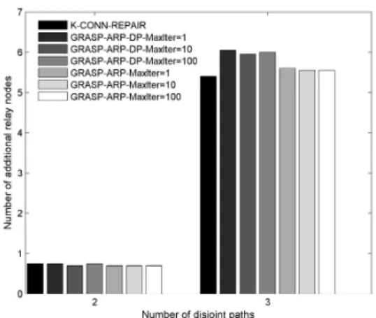
Fig. 1. Number of additional relay nodes needed for the multiple sources -single corner sink in 25-node networks

TABLE II

RELAY PLACEMENT ALGORITHMS’RUN TIME FOR THE MULTIPLE SOURCES-SINGLE CORNER SINK IN25-NODE NETWORKS

Algorithms _kRun time (sec)_{= 2 k= 3}

K-CONN-REPAIR 8.1711 23.5087 GRASP-ARP-DP-MaxIter=1 1.3539 61.7501 GRASP-ARP-DP-MaxIter=10 3.9977 200.3548 GRASP-ARP-DP-MaxIter=100 26.7742 1573.4410 GRASP-ARP-MaxIter=1 1.3032 91.3281 GRASP-ARP-MaxIter=10 4.5867 244.6632 GRASP-ARP-MaxIter=100 36.8587 1814.2370

a network. Our simulation results are based on the mean value of 20 randomly generated network deployments, enough to achieve a 95% confidence interval. The network consists of up to 225 sensor nodes deployed within randomly perturbed grids, where a sensor node is placed in a unit grid of 8m×8m and the coordinates are slightly perturbed. Candidate relays are also distributed in a grid area, where a candidate occupies a unit grid of 4m×4m. Both sensor nodes and relay nodes use the same transmission range, i.e. 10 metres.

We compared GRASP-ARP to the partial k-connectivity repair algorithm (K-CONN-REPAIR for short) proposed by Pu et al. [5]. We followed the algorithm detailed in [5] and made two necessary modifications to work in constrained deployment locations, where relay nodes can only be placed in specific candidate locations. The original K-CONN-REPAIR deploys relay nodes along a straight line between two sensor nodes. Therefore, our first modification is to place relay nodes in candidate locations along the shortest relay path between two sensor nodes. When all relay nodes are deployed, our second modification tries to remove relay nodes one by one by still preserving the k-connectivity. We use a maximum network flow based checking algorithm [15], [16] to check the connectivity. In the simulation, we compared the performance of GRASP-ARP against K-CONN-REPAIR in terms of the number of additional relay nodes needed and the run time.

Fig. 2. Number of additional relay nodes needed for the multiple sources -single centre sink in 25-node networks

TABLE III

RELAY PLACEMENT ALGORITHMS’RUN TIME FOR THE MULTIPLE SOURCES-SINGLE CENTRE SINK IN25-NODE NETWORKS

Algorithms Run time (sec)_{k= 2 k= 3}

K-CONN-REPAIR 8.1711 23.5087 GRASP-ARP-DP-MaxIter=1 1.2009 18.6055 GRASP-ARP-DP-MaxIter=10 3.2695 56.4545 GRASP-ARP-DP-MaxIter=100 29.1741 396.7828 GRASP-ARP-MaxIter=1 1.3203 27.6423 GRASP-ARP-MaxIter=10 4.4375 94.7696 GRASP-ARP-MaxIter=100 42.3155 755.2196

A. Multiple Sources - Single Sink Problem

We choose the sink at the top-left or in the centre of the network, while all sensor nodes are the source nodes. Our simulation uses 25-node topologies and 100 candidate relays. We also set the maximum path length lmax equals to 10

for topologies which consist of 25 sensor nodes. GRASP-ARP uses the dynamic programming implementation (DP) and the basic Counting-Paths algorithm to find the k node-disjoint paths. Figure 1 shows the number of additional relay nodes needed for k= 2 and k= 3 for the case where the sink location is at the top-left of the network, while Figure 2 shows the results for the case where the sink is in the centre. Our GRASP-ARP finds nearly the same number of additional relay nodes compared toK-CONN-REPAIR when the position of the sink is in the centre of the network because it has higher connectivity. These two figures also show that the effect of randomness in GRASP does not guarantee that a higher number of maximum iteration (MaxIter) in the local search produces better results. Table II and III shows the algorithms’ run time, where for small networks, GRASP-ARP takes longer compared to K-CONN-REPAIR especially for k= 3. This happens because GRASP-ARP repeatedly executes Counting-Paths during the local search phase.

B. Multiple Sources - Multiple Sinks Problem

We have four sinks deployed at the top-left, top-right, bottom-left and bottom-right of the network. We use 49-node

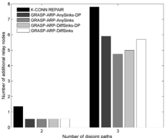
Fig. 3. Number of additional relay nodes needed for the multiple sources -multiple sinks in 49-node networks

TABLE IV

RELAY PLACEMENT ALGORITHMS’RUN TIME FOR THE MULTIPLE SOURCES-MULTIPLE SINKS IN49-NODE NETWORKS

Algorithms Run time (sec)_{k= 2 k= 3}

K-CONN-REPAIR 283.5649 665.4548 GRASP-ARP-AnySinks-DP 30.1625 274.1320 GRASP-ARP-AnySinks 38.0461 387.7298 GRASP-ARP-DiffSinks-DP 23.8539 336.0117 GRASP-ARP-DiffSinks 42.2258 426.7554

topologies with 196 candidate relays and set lmax equals to

15. In multiple sinks problem, there are two cases where the node-disjoint paths terminate at:different sinksandany sinks. The different sinks problem is where theknode-disjoint paths must terminate at k different sinks. The any sinks problem is the case where the k node-disjoint paths may terminate at any sinks. Figure 3 and Table IV show the simulation results, where we usemax iteration= 10 for GRASP-ARP. In this scenario, GRASP-ARP outperforms K-CONN-REPAIR in both the number of additional relay nodes needed and the run time because GRASP-ARP only findsk node-disjoint paths to the dedicated sinks, while K-CONN-REPAIR must run an expensive connectivity checking algorithm in each iteration to provide k-connectivity for an entire network.

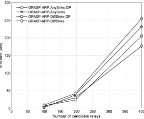
We also vary the number of candidate relays in the networks to show whether it has an impact on the run time efficiency of GRASP-ARP. As depicted in Figure 4 for the 49-node networks, the run time increases significantly when the number of candidate relays increases.

K-CONN-REPAIR is too costly to be implemented in a larger network as it needs to check the connectivity between every pair of nodes. Our GRASP-ARP, on the other hand, is able to scale larger networks. We present the run time for 100 and 225-node topologies in Table V. The results presented here are fork= 2and use 400 candidate relays, where 100 and 225-node networks need 0.7 and 1.45 additional relay nodes in average, respectively. More simulation results are available in [14].

Fig. 4. Algorithms’ run time in increasing number of candidate relays for the multiple sources - multiple sinks in 49-node networks

TABLE V

RELAY PLACEMENT ALGORITHMS’RUN TIME FOR THE MULTIPLE SOURCES-MULTIPLE SINKS IN100AND225-NODE NETWORKS

Algorithms Run time (sec) 100-node 225-node

GRASP-ARP-AnySinks-DP 269.2118 834.9906 GRASP-ARP-AnySinks 307.9353 1358.7140 GRASP-ARP-DiffSinks-DP 261.9937 1027.2200 GRASP-ARP-DiffSinks 305.1702 1245.4740

VI. CONCLUSION ANDFUTUREWORK

Ensuring that wireless sensor networks are robust to fail-ures requires that the physical network topology will offer alternative routes to the sink. This requires sensor network deployment to be planned with an objective of ensuring some measure of robustness in the topology, so that when failures do occur that routing protocols can continue to offer reliable delivery. Our contribution is a solution that enables fault-tolerant WSN deployment planning by judicious use of additional relay nodes. In this paper, we define the problem for increasing WSN reliability by deploying a number of additional relay nodes to ensure that each sensor node in the initial design has k node-disjoint paths to the sinks. We present GRASP-ARP, a centralised offline algorithm to be run during the initial topology design to solve this problem. We also adapt a version of the closest approach from the literature for comparison. Our simulation results show that our solution requires fewer relay nodes for larger problems than the competitor, and that different variants of our algorithm are significantly faster, allowing us to tackle larger problems.

We are currently evaluating network protocols and opera-tions using the designed topologies in the network simulator ns-2. While this paper focuses on additional relay node ployment, our future work will include additional sensor de-ployment, as well as finding locations to deploy sinks in a hop-constrained network that can optimise the network resiliency. We will also consider the networks capacity requirement in the algorithm design.

ACKNOWLEDGMENT

This research is fully funded by the NEMBES project, supported by the Irish Higher Education Authority PRTLI-IV research program.

REFERENCES

[1] D. Torrieri, “Algorithms for Finding an Optimal Set of Short Disjoint Paths in a Communication Network,”IEEE Transactions on Communi-cations, vol. 40, no. 11, pp. 1698–1702, 1992.

[2] T. Feo and M. Resende, “Greedy Randomized Adaptive Search Proce-dures,”Journal of Global Optimization, vol. 6, pp. 109–133, 1995. [3] B. Hao, J. Tang, and G. Xue, “Fault-Tolerant Relay Node Placement in

Wireless Sensor Networks: Formulation and Approximation,” inProc. Workshop High Performance Switching and Routing (HPSR’04), 2004, pp. 246–250.

[4] J. Bredin, E. Demaine, M. Hajiaghayi, and D. Rus, “Deploying Sensor Networks with Guaranteed Capacity and Fault Tolerance,” in Proc. 6th ACM Int’l Symp. Mobile Ad Hoc Networking and Computing (MobiHoc’05), 2005, pp. 309–319.

[5] J. Pu, Z. Xiong, and X. Lu, “Fault-Tolerant Deployment with k -connectivity and Partial k-connectivity in Sensor Networks,”Wireless Communications and Mobile Computing, vol. 9, no. 7, pp. 909–919, 2008.

[6] A. Kashyap, S. Khuller, and M. Shayman, “Relay Placement for Fault Tolerance in Wireless Networks in Higher Dimensions,”Computational Geometry, 2010.

[7] X. Han, X. Cao, E. Lloyd, and C. Shen, “Fault-tolerant Relay Node Placement in Heterogeneous Wireless Sensor Networks,” IEEE Trans. Mobile Computing, vol. 9, no. 5, pp. 643–656, 2010.

[8] W. Zhang, G. Xue, and S. Misra, “Fault-Tolerant Relay Node Placement in Wireless Sensor Networks: Problems and Algorithms,” inProc. 26th Ann. IEEE Conf. Computer Communications (INFOCOM’07), 2007, pp. 1649–1657.

[9] S. Misra, S. Hong, G. Xue, and J. Tang, “Constrained Relay Node Placement in Wireless Sensor Networks to Meet Connectivity and Survivability Requirements,” inProc. 27th Ann. IEEE Conf. Computer Communications (INFOCOM’08), 2008, pp. 281–285.

[10] R. Bhandari, “Optimal Physical Diversity Algorithms and Survivable Networks,” inProc. 2nd IEEE Symp. Computers and Communications (ISCC’97), 1997, pp. 433–441.

[11] L. Ford and D. Fulkerson,Flows in Networks. Princeton, University Press, 1962.

[12] J. Kleinberg and E. Tardos,Algorithm Design. Addison-Wesley, 2011. [13] S. Martins, P. Pardalos, M. Resende, and C. Ribeiro, “Greedy Random-ized Adaptive Search Procedures for the Steiner Problem in Graphs,” in

Randomization Methods in Algorithmic Design, ser. DIMACS Series on Discrete Mathematics and Theoretical Computer Science. American Mathematical Society, 1999, vol. 43, pp. 133–145.

[14] L. Sitanayah, K. Brown, and C. Sreenan, “Relay Node Placement for k Node-Disjoint Paths in Constrained Wireless Sensor Network Deployment Planning,” Dept. of Computer Science, University College Cork, Tech. Rep. UCC-CS-2011-07-17, Jul. 2011.

[15] C. Papadimitriou and K. Steiglitz,Combinatorial Optimization: Algo-rithms and Complexity. Englewood Cliffs, NJ: Prentice Hall, 1982. [16] R. Ravi and D. Williamson, “An Approximation Algorithm for

Minimum-Cost Vertex-Connectivity Problems,”Algorithmica, vol. 18, no. 1, pp. 21–43, 1997.