When and Why Are They Beneficial?
Christiane Lemke
A thesis submitted in partial fulfilment of the requirements of Bournemouth University for the degree of Doctor of Philosophy
January 2010
This copy of the thesis has been supplied on condition that anyone who consults it is understood to recognise that its copyright rests with its author and due acknow-ledgement must always be made of the use of any material contained in, or derived from, this thesis.
Time series forecasting has a long track record in many application areas. In forecas-ting research, it has been illustrated that finding an individual algorithm that works best for all possible scenarios is hopeless. Therefore, instead of striving to design a single superior algorithm, current research efforts have shifted towards gaining a deeper understanding of the reasons a forecasting method may perform well in some conditions whilst it may fail in others. This thesis provides a number of contribu-tions to this matter. Traditional empirical evaluacontribu-tions are discussed from a novel point of view, questioning the benefit of using sophisticated forecasting methods without domain knowledge. An own empirical study focusing on relevant off-the-shelf forecasting and forecast combination methods underlines the competitiveness of relatively simple methods in practical applications. Furthermore, meta-features of time series are extracted to automatically find and exploit a link between application specific data characteristics and forecasting performance using meta-learning. Fi-nally, the approach of extending the set of input forecasts by diversifying functional approaches, parameter sets and data aggregation level used for learning is discussed, relating characteristics of the resulting forecasts to different error decompositions for both individual methods and combinations. Advanced combination structures are investigated in order to take advantage of the knowledge on the forecast generation processes.
Forecasting is a crucial factor in airline revenue management; forecasting of the anticipated booking, cancellation and no-show numbers has a direct impact on gene-ral planning of routes and schedules, capacity control for fareclasses and overbooking limits. In a collaboration with Lufthansa Systems in Berlin, experiments in the the-sis are conducted on an airline data set with the objective of improving the current net booking forecast by modifying one of its components, the cancellation forecast. To also compare results achieved of the methods investigated here with the current state-of-the-art in forecasting research, some experiments also use data sets of two recent forecasting competitions, thus being able to provide a link between academic research and industrial practice.
Copyright statement ii
Abstract iii
List of Tables vii
List of Figures ix
Acknowledgements x
Author’s declaration xi
List of Abbreviations and Symbols xii
1 Introduction 1
1.1 Background and motivation . . . 2
1.2 Aims and objectives . . . 3
1.3 Methodology and organisation of the thesis . . . 4
1.4 Original contributions . . . 5
1.5 List of publications . . . 5
2 Airline revenue management and forecasting 7 2.1 Airline revenue management . . . 7
2.1.1 Background . . . 7
2.1.2 History . . . 9
2.1.3 The role of forecasting . . . 10
2.1.4 Lufthansa Systems forecasting basics . . . 10
2.1.5 Lufthansa Systems cancellation forecasting . . . 13
2.2 Time series forecasting . . . 17
2.2.1 Exponential smoothing . . . 17
2.2.2 ARIMA models . . . 18
2.2.3 State-space models . . . 19
2.2.4 Regime switching . . . 19
2.2.5 Artificial neural networks . . . 20
2.3 Forecast combinations . . . 21
2.3.1 Nonparametric methods . . . 22
2.3.2 Variance-covariance based methods . . . 22
2.3.3 Regression . . . 23
2.3.4 Nonlinear combinations . . . 24
2.3.5 Adaptivity . . . 27
2.3.6 Combining or not combining? . . . 28
2.4 Chapter summary and future work . . . 29
3 Do we need experts for time series forecasting? 31 3.1 Choosing a forecasting approach . . . 31
3.1.1 Empirical studies . . . 31
3.1.2 Evidence on using combinations of forecasts . . . 33
3.1.3 Conclusions . . . 34
3.2.1 Data sets . . . 35 3.2.2 Methodology . . . 36 3.2.3 Results (single-step-ahead) . . . 41 3.2.4 Results (multi-step-ahead) . . . 41 3.2.5 Outcomes . . . 44 3.3 Chapter summary . . . 46
4 Forecast combination for airline data 47 4.1 Data set and methodology . . . 47
4.2 Individual forecasting methods . . . 49
4.3 Combinations . . . 52
4.4 Conclusions . . . 53
5 Meta-learning 55 5.1 Background . . . 55
5.2 Methodology for empirical studies . . . 57
5.2.1 Exploratory analysis . . . 58
5.2.2 Comparing meta-learning approaches . . . 58
5.3 Meta-learning for competition data . . . 60
5.3.1 Time series features . . . 60
5.3.2 Exploratory analysis - decision trees . . . 65
5.3.3 Comparing meta-learning approaches . . . 67
5.3.4 Ranking in the NN5 competition . . . 69
5.4 Meta-learning for the airline application . . . 69
5.4.1 Exploratory analysis - the data . . . 70
5.4.2 Global meta-learning . . . 73
5.4.3 Local meta-learning . . . 74
5.5 Chapter summary . . . 75
6 Diversification strategies for the airline application 78 6.1 Background and motivation . . . 78
6.1.1 The ambiguity decomposition . . . 79
6.1.2 Bias/variance/covariance . . . 80
6.1.3 Motivation for diversification . . . 81
6.2 Generating forecasts by diversification procedures . . . 82
6.2.1 Decomposing data . . . 82
6.2.2 Diversifying functional approaches . . . 83
6.2.3 Diversifying parameters . . . 83
6.2.4 Diversifying training data . . . 84
6.2.5 Summary . . . 85
6.3 Application-specific dynamics of the error components . . . 85
6.3.1 The interaction with the booking forecast . . . 85
6.3.2 Aggregating . . . 86
6.4 Flat combinations of diversified forecasts . . . 86
6.4.1 Diversifying level of learning . . . 86
6.4.2 Diversifying the smoothing parameter . . . 89
6.5 Advanced combination techniques . . . 91
6.5.1 Pooling and multilevel structures . . . 91
6.5.2 Evolving multilevel structures . . . 93
6.5.4 Results . . . 95
6.5.5 Analysis of generated structures . . . 98
6.6 Chapter summary . . . 101
7 Conclusions and future work 103 7.1 Summary of the chapters . . . 103
7.2 Findings and conclusions . . . 104
7.3 Original contributions . . . 105
7.4 Future work . . . 106
A Description of the software 107 A.1 Preprocessing . . . 107
A.1.1 ABS TO RATE and RATE TO ABS . . . 107
A.1.2 CONSTRAIN RATE . . . 108
A.1.3 UNCONSTRAINING CANC . . . 108
A.2 Data analysis . . . 108
A.2.1 DEFAULT PROB . . . 108
A.2.2 DATA ANALYSE . . . 109
A.2.3 FEATURES . . . 109
A.3 History building . . . 109
A.3.1 HB SMCANC . . . 109 A.3.2 HB REGRCANC . . . 110 A.3.3 HB PROBCANC . . . 110 A.4 Forecasting . . . 111 A.4.1 FC CANC . . . 111 A.4.2 FC PROBCANC . . . 111 A.4.3 FC META . . . 112
B Airline data experiments 113
2.1 Days to departure for each data collection point (DCP). . . 11
2.2 Simplified example of a cancellation probability reference curve. . . . 16
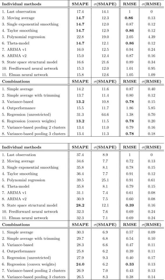
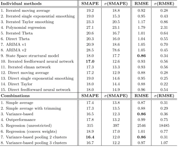
3.1 Forecast performances and standard deviation on NN3 data (top) and NN5 data (bottom), single-step-ahead . . . 42
3.2 Forecast performances and standard deviation on NN3 data (SMAPE), multi-step-ahead . . . 43
3.3 Forecast performances and standard deviation on NN5 data, multi-step-ahead . . . 44
4.1 Mean absolute deviation of reference net booking forecast and per-centage of relative improvement of four individual forecasting algo-rithms for each DCP. Left: high aggregation level, right: low aggre-gation level. . . 50
4.2 Mean absolute deviation of reference cancellation forecast and per-centage of relative improvement of four individual forecasting algo-rithms for each DCP. Left: high aggregation level, right: low aggre-gation level. . . 51
4.3 Flat forecast combination: percentage of relative performance im-provement compared to reference forecast (lsb), high level . . . 52
4.4 Flat forecast combination: percentage of relative performance im-provement compared to reference forecast (lsb), low level . . . 53
5.1 Time series model selection - overview of literature . . . 57
5.2 Summary of features - general statistics . . . 62
5.3 Summary of features - frequency domain . . . 62
5.4 Summary of features - autocorrelations . . . 63
5.5 Summary of features - diversity . . . 64
5.6 Label sets for the meta-learning classification problem . . . 68
5.7 SMAPE error measures applying three classic meta-learning techniques 68 5.8 SMAPE error measures applying the meta-learning ranking algorithm 69 5.9 Performances applying different meta-learning techniques, competi-tion condicompeti-tions . . . 69
5.10 Airline data features summary statistics . . . 71
5.11 Correlation coefficients of airline data features and net booking errors 72 5.12 Global meta-learning: percentage of relative performance improve-ment compared to reference forecast, high level . . . 73
5.13 Global meta-learning: percentage of relative performance improve-ment compared to reference forecast, low level . . . 74
5.14 Local meta-learning: percentage of relative performance improvement compared to reference forecast, high level . . . 75
5.15 Local meta-learning: percentage of relative performance improvement compared to reference forecast, low level . . . 76
6.1 Level diversification: percentage of relative performance improvement compared to reference forecast, top: high level, bottom: low level . . 88 6.2 Parameter diversification: percentage of relative performance
6.3 Percentage of relative net booking forecast improvement of combina-tion structures compared to the reference forecast. Top: parameter and level diversified forecasts, bottom: parameter diversified fore-casts, left: high aggregation level, right: low aggregation level. . . 96 6.4 Percentage of relative net booking forecast improvement of
combi-nation structures compared to the reference forecast using the im-proved booking forecast. Top: parameter and level diversified fore-casts, bottom: parameter diversified forefore-casts, left: high aggregation level, right: low aggregation level. . . 97 6.5 Mapping of forecast representations in the figures to the actual
fore-cast generation . . . 98 6.6 Percentage of times a particular combination method is present in the
final evolved structure in ev1 and ev4 . . . 100 6.7 Percentage of times an individual forecast is present in the final
struc-ture in ev1 . . . 100 6.8 Percentage of times a particular aggregation dimension is selected for
2.1 Interaction of forecasting with optimisation and past booking numbers 10 2.2 Example of reference curves, bookings (left) and cancellation rate
(right), values given for each of the 23 DCPs prior to departure. . . 12
2.3 Reference curve and confidence limits . . . 14
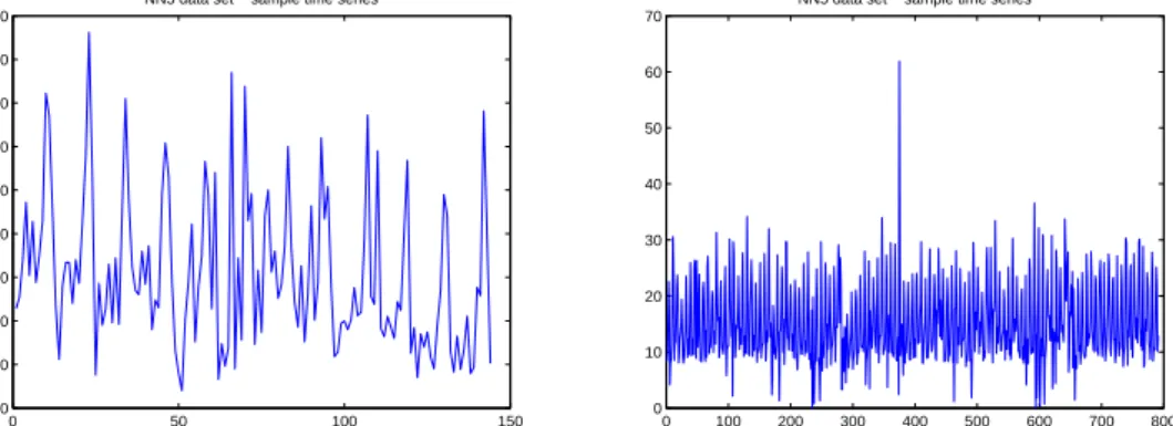
3.1 Examples of time series, left: NN3 competition, right: NN5 competition. 36 3.2 Histogram showing number of series for which a method performed best, left: NN3 competition, right: NN5 competition. . . 45
3.3 Histogram showing number of series for which a combination method performed best (SMAPE), left: NN3 competition, right: NN5 com-petition. . . 45
4.1 Steps and components of the cancellation forecasting procedure. . . 48
4.2 Example of the relation between booking, cancellation and net book-ing errors, left: a cancellation forecast with a higher error leadbook-ing to a better net booking forecast because it compensates the booking error, right: a cancellation forecast with a lower error leading to worse net booking forecast because compensation does not have the same extent. 51 5.1 Meta-learning overview . . . 58
5.2 Decision tree one - which individual method? . . . 66
5.3 Decision tree two - which combination method? . . . 66
5.4 Decision tree three - which method? . . . 67
5.5 Average performance in relation to number of clusters . . . 68
5.6 Decision tree - best method for airline net booking forecast . . . 72
6.1 Decomposition of data in the airline application . . . 83
6.2 Example of different aggregation levels of airline data . . . 85
6.3 Reference curves learnt on high level and low level and actual data averaged per calendar week. Left: scenario in which the low level curve corresponds to data much better, right: scenario where higher level information can be beneficial towards the end . . . 87
6.4 Average cancellation forecast errors, with the different curves corre-sponding to three different parameters used, smoothing factor (left) and confidence limit width (right). . . 89
6.5 Example of a combination structure generated by variance-based pool-ing . . . 92
6.6 Illustration of a combination structure generated by dimension-specific pooling . . . 93
6.7 Sample combination structure generated by the ev1 algorithm . . . . 99
To Bogdan: Thank you for being a great supervisor. For enabling me to get to know life in academia in all of its facets and providing interesting perspectives for the future. For motivating me and believing in me when I needed it. Your help, time and dedication are greatly appreciated.
To Silvia: Thank you for constant encouragement and your enthusiasm regarding the airline application of this work. For providing me a practical perspective and not letting me get lost in exclusively academic thoughts.
To my parents, sister and grandparents: Thank you for your unconditional love and support, as well as putting up with my ideas, which might have seemed crazy at times. I will probably keep them coming.
To my fellow PhD students: Thank you for making my time at Bournemouth Uni-versity a very pleasant one, it was great getting to know and working with you. To my friends in the UK: Vegard, thank you for going the better part of the PhD journey with me. For helping me overcome the little chicken inside of me at various occasions and for bearing with me when I banned PhD and work talk from con-versations. Janko, thank you for your support during the crazy final PhD stages. I keep being amazed by how much we think alike and how you manage to make me feel happy. Kasia, I am so glad we met. Thank you for all the basketball, the conversations we had and for believing in me all the time. Isla, thank you for being genuine and bubbly and for getting me away from my computer to do fun stuff like climbing and kitesurfing.
To my friends “from home”: Jana, thank you for being the strongest link to my life in Germany. Our telephone chats in good and bad times are one of my weekly highlights. Julia, thank you for your contagious restlessness and for the fun times we have whenever we meet. Ulli, thank you for being an inspiration with your un-usually honest and emotional personality. Ralf, thank you for being so direct and our refreshingly blunt conversations. Lars, thank you for showing me the world of poetry slams and the beautifully melancholic hours we spend playing the guitar. I would also like to thank Bournemouth University and Lufthansa Systems Berlin for the support and for providing a productive and enjoyable research and work environment.
The work contained in this thesis is the result of my own investigations and has not been accepted nor concurrently submitted in candidature for any other award. Conference and journal publications related to this work are referenced. This thesis has been conducted in a collaboration with Lufthansa Systems Berlin GmbH and continues work of a previous project that resulted in the thesis of Riedel (2007).
ARIMA Autoregressive integrated moving average ARR Adjust ratio of ratios
DCP Data collection point
DOW Day of the week
DT Decision tree
F Fareclass
GMDH Group method of data handling LSB Lufthansa Systems Berlin GmbH
MSE Mean squared error
NN Neural networks
NN3/NN5 Neural network forecasting competitions 2006/2008 O&D Origin and destination pair
ODO Origin-destination opportunity
POS Point of sale
RMSE Square root of the mean squared error S Seasonal component of a time series
SETAR Self-exciting threshold autoregressive models SMAPE Symmetric mean absolute percentage error STAR Smooth transition autoregressive models
SVM Support vector machine
T Trend component of a time series
α, β, γ Smoothing parameters for smoothing based approaches
ˆ
y Vector of time series forecasts
ω Combination weight vector
e Unity vector
Forecast error
ˆ
y Time series forecast
ˆ
yc Combined time series forecast
ω Weights for linear forecast combination
φ Dampening factor
P
Covariance matrix
b Bookings
cr Cancellation rate
ref Reference curve in the airline application
f Feature
l Level of a time series
r Growth rate of a time series
t Trend of a time series
1
Introduction
Going beyond the well-known daily weather forecast, forecasts can be found in a wide variety of scenarios. Forecasting stock prices and exchange rates is common practice in finance as, for example, investigated in Gyorfi et al. (2006) and Kodogiannis & Lolis (2002). Forecasting variables like gross national product or unemployment is crucial for macroeconomics, for a recent example see Marcellino et al. (2006). As demonstrated in Weatherford & Kimes (2003) and Koutroumanidis et al. (2009), companies of all sizes use forecasts to predict demand for their products to support planning and decision-making. The lead time for decisions can vary significantly depending on the application; electrical load applications as described in Hippert et al. (2005) may require forecasts every few seconds while a few days are usually sufficient for transportation and production schedules as, for example, investigated in Cox Jr & Popken (2002). In the case of long-term investments based on macroe-conomic data as used by Stock & Watson (2002), lead time can even amount to several years.
In general, forecasting describes a broad research area concerned with estimation of future events or conditions. According to Makridakis et al. (1998), forecasting approaches can be roughly divided into qualitative and quantitative models. Qua-litative models assume sufficient knowledge of an underlying process and are often experts’ judgements. Experts usually base their opinion on different sources of in-formation, their intuition and subjective beliefs that cannot be easily quantified. The focus of this thesis however lies on quantitative forecasting, which mainly in-volves automatic prediction of numerical data. The data examined here consists of univariate sequences of data points, so called time series, that are investigated for regularities and patterns in their past to extract knowledge that can help to predict the future. In addition to looking at data sets publicly available from forecasting competitions, data has been provided by Lufthansa Systems Berlin GmbH (LSB), allowing an investigation of forecasting approaches in the industrial setting of the airline industry.
This chapter will give background information and motivations for this work. It will start to set the scene for the airline-specific part of the thesis by describing the importance of forecasting in the context of airline revenue management. It will continue to introduce the area of time series forecasting in general, including a brief look at forecast combinations and meta-learning, which are major topics in this thesis. The definition of aims and objectives as well as a description of the organisation of the thesis follow in the next sections. An overview of the original contributions and a list of publications conclude the chapter.
1.1 Background and motivation
A considerable part of the work presented in this thesis has been carried out in collaboration with Lufthansa Systems Berlin GmbH, a company providing revenue management software for airline carriers. The products the airline industry offers are seats on a plane which, contrary to the perception on first sight, do not only differ in being in the physically separated first or second class. Pak & Piersma (2002) rather describe it as a complex system of fareclasses that differ in various conditions, like refund availabilities, cancellation options or stopover arrangements. Customers can roughly be separated in two groups according to Zeni (2001): business and leisure passengers. While business passengers usually seek to make travel arrangements shortly before departure with little flexibility, leisure passengers tend to book their tickets well in advance while being more flexible with dates and booking conditions. In addition, business passengers are usually willing to pay a higher price for their tickets, thus contributing to more revenue than a leisure customer. The key to efficient capacity control is the determination of the point in time when it is beneficial to restrict bookings in a lower-fare class to leave space for later booking high-fare customers. This is of both economical and ecological interest, producing a higher revenue for a high demand flight and fewer unoccupied seats in a low demand one. Accurate forecasting of anticipated booking, cancellation and no-show numbers is vital for revenue management. If the demand forecast of high-fare passengers is too high, seats go empty that could have been sold to low-fare passengers. On the other hand, if it is too low, passengers willing to pay a higher fare have to be turned away. Revenue management and forecasting do however not only support the decisions that have to be made on a daily basis, but also provide key information for strategic long-term decisions such as which itineraries to offer or how to change the size of the maintained fleet, see Zaki (2000).
Historic booking and cancellation numbers constitute time series, which might include valuable information for forecasting the future. Time series forecasting has been a very active area of research since the 1950’s, and a variety of forecasting approaches have been introduced in the scientific literature and were used in many practical applications. Available forecasting algorithms can be roughly divided into a few groups: simple approaches are often surprisingly robust and popular, for example those based on exponential smoothing. Statisticians and econometricians tend to rely on complex ARIMA models and their derivatives, while the machine learning community mainly looks at neural networks. A review can be found in Gooijer & Hyndman (2006).
A few years after the first publications in the area of time series forecasting, research on combinations of forecasts became popular as well, with the seminal pa-per having been published by Bates & Granger (1969). It divided the community into researchers who believe that combinations are a great approach to decrease the risk of selecting the wrong individual model and better approximating a real world time series, and others who think that if a combination outperforms indi-vidual methods, it is only an indication of an indiindi-vidual method requiring better specification. However, especially in machine learning, combinations of methods have proven successful. As summarised in the review of Timmermann (2006), the choice of combination methods is extensive. Very simple methods average available individual forecasts with or without a certain degree of trimming, others take past
performance into account in different ways for calculating linear weights. Nonlinear forecast combination methods do exist, but literature seems comparatively sparse.
During the years, more focus has been put on the question of when a particular forecasting method works well. Promising work has been published on linking cha-racteristics of time series to the performance of a forecasting algorithm, first mostly in the context of rule based systems as, for example, in Adya et al. (2001). More recently, the term “meta-learning” was adopted from the machine learning commu-nity, accommodating a wider range of learning methods as described in Prudencio & Ludermir (2004a) and Wang et al. (2009).
In a previous collaboration project resulting in the thesis of Riedel (2007), diver-sification procedures to extend the number of available individual forecasts similar to the ones introduced in Granger & Jeon (2004) have been investigated and applied to demand forecasting for airline data. The success of the work led to the belief that higher overall forecast accuracy can also be achieved by modifying the cancellation forecast, which is another important component in airline revenue management fore-casting and which will be investigated in this thesis. Aims and objectives of this thesis in general and for the airline application in particular are described in the next section.
1.2 Aims and objectives
The main aim of the thesis is contributing to a better understanding of forecast model selection and combination approaches. On a general level, the following questions will be investigated:
• To what extent are expert contributions beneficial in empirical forecasting applications? Can adequate performance be achieved by combining simple individual predictors?
• How can a pool of individual methods be extended, and what characteristics are necessary to increase combination accuracy?
• Can situations in which a particular method works well be automatically iden-tified and domain knowledge exploited for improved forecasting performance? A major practical goal of this thesis is the improvement of the net booking forecast in the airline revenue management application of Lufthansa Systems by looking at modifications for one of its components, the cancellation forecast. To achieve this, several objectives are pursued:
• The design and implementation of a new forecast based on cancellation prob-abilities, enhancing the diversity of the individual forecasts available for com-bination.
• Investigation of the benefit of forecast combination for airline data and the ex-tent of possible improvements while meeting application-specific requirements like time restrictions and coping with noisy data.
• Automatically generating and exploiting domain knowledge for method selec-tion and more effective combinaselec-tion of individual predictors.
• Evaluation of diversification procedures for generating additional individual forecasts, by considering different functional approaches, different parametri-sations and different aggregation levels of the data used for learning.
To achieve these contributions, relevant literature will be reviewed and discussed before conducting and analysing empirical investigations. Two different kinds of data sets will be used for increased value of the results: publicly available data sets obtained from forecasting competitions will allow comparison of the results given in this thesis to results obtained by experts in the field of time series forecasting and facilitate replication. The application of the investigated approaches to real-world airline data will give insights to the applicability of latest research results to an industry, in which accurate time series forecasting has a big impact on generated revenue.
1.3 Methodology and organisation of the thesis
Background knowledge in three different areas are relevant for this thesis: airline revenue management, time series forecasting and forecast combination. The intro-ductory information will be extended in Chapter 2, providing a literature review and discussion of most important contributions and algorithms for each of the areas.
Chapter 3 investigates the question of how well off-the-shelf time series fore-casting methods perform in empirical studies with the goal to assess the benefit of applying complex forecasting algorithms that usually have to be identified and fitted by experts. In the same context, the benefit of combinations of these simple fore-casts, promising to provide a convenient way out of the dilemma of having to find and parametrise a suitable method for each forecasting problem is evaluated. After reviewing evidence from other empirical studies, an experiment designed for this specific point of view is presented and analysed, using publicly available datasets from forecasting competitions to allow comparison with contributions of different experts in the field. Chapter 4 then looks at forecasting methods currently used in the airline application and compares results obtained to those from the previous chapter.
Having provided the background and first empirical results of time series forecas-ting and combination approaches, the focus of this thesis shifts from investigaforecas-ting
which methods work best towhy some methods work well, and in which situations. Chapter 5 considers the forecasting problem from a higher level point of view. It investigates the automatic generation of domain knowledge to guide method selec-tion and combinaselec-tion in the forecasting process, which can be summarised with the term of “meta-learning”. Following an extensive review of work done in this parti-cular area, different machine learning approaches are tested in an empirical study to evaluate possible performance improvements on all the data sets available.
Chapter 6 provides a thorough investigation of opportunities to increase forecast accuracy in the airline application. It looks at characteristics of individual forecasts that are necessary to contribute to an improved combination result, investigating the concept of diversity in the context of pools of time series forecasts. The benefits of functional, parameter and data aggregation level diversification is empirically evaluated and analysed using the airline data set.
Chapter 7 concludes by summarising results and findings and evaluating how the analysis of diversity and meta-learning has contributed to the understanding of forecast combination in general. An outlook on future work ends the thesis.
1.4 Original contributions
A comprehensive treatment of time series forecasting in airline revenue management is given in Chapters 4 and 6 and parts of Chapters 2 and 5, a treatment which has not been yet available in comparable detail. Data used for related empirical studies was kindly provided by Lufthansa Systems, and with airline revenue management applications being an extremely successful practical application area for time series forecasting algorithms, the thesis provides unique insights to the practical relevance of forecasting methods in this area. It complements the thesis of Riedel (2007), which resulted from the same collaboration in a previous project. A new algorithm for the prediction of airline cancellation rates is presented in Chapter 2.
A new perspective on empirical studies and the necessity of expert contribu-tions in practical forecasting applicacontribu-tions is given in Chapter 3, parts of which were published in Lemke & Gabrys (2007), Lemke & Gabrys (2008a) and Ruta et al. (2009).
The meta-learning discussion and empirical study in Chapter 5 is one of the most extensive works in this area to date, extending the features and method pool in comparison to previous work and reviewing a wider range of algorithms. Noteworthy is the use of diversity measures as inputs to the meta-learning algorithms, an original extension to meta-learning in a time series context. Some results have been published in Lemke & Gabrys (2009). The concept of meta-learning is furthermore applied to airline data for the first time.
Diversity is a concept that has its origin in the machine learning community and has not yet to the same extent been applied to time series forecast combina-tion. Chapter 6 looks at the benefit of generating additional individual forecasts by diversifying procedures with the goal to improve the overall accuracy of a forecast combination. Parameter and functional diversifications are most common in the li-terature, this thesis additionally considers individual forecasts generated by building models on different data aggregation levels. Results on a smaller data set have been published in Lemke et al. (2009).
Overall, this thesis does not aim at adding just another method to the already large pool of available forecast and forecast combination approaches, thus increa-sing confusion of which method to chose in which situation. It is rather aimed at providing a deeper understanding of the dynamics of a combination of individual forecasts and of the value of domain knowledge and its automatic generation, which will contribute to knowledge on forecasting in general and facilitate improvements of forecast accuracy.
1.5 List of publications
A list of the publications resulting from this thesis in chronological order is provided below:
• Lemke, C. & Gabrys, B. (2007), Review of nature-inspired forecast combina-tion techniques, in ‘NiSIS 2007 Symposium’
• Lemke, C. & Gabrys, B. (2008a), Do we need experts for time series forecas-ting?, in ‘Proceedings of the 16th European Symposium on Artificial Neural Networks’, pp. 253-258
• Lemke, C. & Gabrys, B. (2008b), On the benefit of using time series features for choosing a forecasting method, in ‘Proceedings of the European Symposium on Time Series Prediction’, pp. 1-10
• Lemke, C. & Gabrys, B. (2009), ‘Meta-learning for time series forecasting and forecast combination’, accepted to a special issue of Neurocomputing
• Lemke, C., Riedel, S. & Gabrys, B. (2009), Dynamic combination of forecasts generated by diversification procedures applied to forecasting of airline can-cellations, in ‘Proceedings of the IEEE Symposium Series on Computational Intelligence’, pp. 85-91
• Ruta, D., Gabrys, B. & Lemke, C. (2009), ‘A generic multilevel architecture for time series prediction’, accepted to IEEE Transactions on Knowledge and Data Engineering
2
Airline revenue management and forecasting
The introduction presented forecasting as an important topic in both research and industrial applications. However, the state-the art in industry and research of-ten differ quite significantly for several reasons: sometimes research findings are purely academical and cannot easily be applied in real-world applications; or the requirement for robust and reliable systems in industry causes a certain reluctance to implement latest research outcomes. Furthermore, there is never a guarantee that approaches working well or badly on scientific data sets will perform similarly on data sets in industrial applications, especially since industrial data sets are usually hard to come by in the public domain for reasons of commercial sensitivity. This chapter provides an overview of the state-of-the art in forecasting algorithms from both a scientific perspective as well as from the point of view of the industry partner of this work.
Following an introduction to revenue management, the first section of this chap-ter highlights the importance of forecasting in the airline industry in particular and introduces forecasting algorithms used at Lufthansa Systems Berlin GmbH (LSB). The next sections take a step away from the specific application and provide a look at time series forecasting and forecast combination in general. A presentation of the most important algorithms is followed by an outlook on future work.
2.1 Airline revenue management
Revenue management has become a mainstream business practice with a growing importance in academic and industrial research and an increasing number of users in many key industries according to Talluri & van Ryzin (2005). Its goal is to maximise profits generated from limited perishable resources by optimising demand-related decisions, thus selling the right product to the right customer at the right time for the right price. Perishable resources can be as diverse as food, hotel rooms or train tickets.
This section extends the introductory information given on revenue management. Its significance particularly for the airline industry is emphasised in a brief historical overview showing that airlines were the first and remain one of most successful users of these systems till today. A look at the role of forecasting in revenue management then provides the connection to the presentation of forecasting methods currently used.
2.1.1 Background
The basic concept of revenue management is very old. However, Talluri & van Ryzin (2005) mention two factors that have considerably boosted its potential in
the last 50 years: scientific advances that facilitate more accurate models of real-world conditions and advances in information technology, that allow use of very complex algorithms on a very detailed level if necessary. This made way for modern automated revenue management on a very high scale and complexity. Revenue management is concerned with four major components: pricing, capacity control, overbooking and forecasting:
Pricing investigates the time-varying calculation of prices for a product. Usually, there is not only one product for one group of customers, but a portfolio of products targeting different customer groups. According to McGill & van Ryzin (1999), pri-cing is generally the most important and natural factor affecting customer demand behaviour and can be used to manipulate demand in the short run. For example, sufficiently raising the price of one product class will result in sales of this product approaching zero. A review of research done in the area of dynamic pricing policies in the context of revenue management can be found in Bitran & Caldentey (2003). Capacity control manages the allocation of capacities within the bundle of pro-ducts. It commonly distinguishes single-resource problems, where the goal is to optimally allocate capacities for a single resource to different classes of demand, and multiple-resource problems, where customers require a combination of resources, for example in a stay in a hotel lasting several days. If one product in the pro-duct bundle is not available, the sales of the whole bundle is affected, creating the need of jointly managing resources. Talluri & van Ryzin (2005) state that although multiple-resource problems are much more common in the industrial practice of reve-nue management, they are still often solved as a number of single-resource problems, treating the resources independently and ignoring network effects that might occur. Usual means for capacity control are limits, specifying how many products from a product class may be sold at most, or protection levels, reserving an amount of capacity for a particular class.
Overbooking is the oldest practice in revenue management and can only be ap-plied in reservation-based systems. Its goal is to compensate for cancellations and no-shows by accepting more reservations than the capacity allows, hoping that the number of customers actually claiming the service or product will be within the capacity. An obvious danger in this respect is the chance of more customers turning up than anticipated, which means that additional revenue generated by overbooking is to be traded off against the risk and compensation of having to deny a service or product. According to Talluri & van Ryzin (2005), overbooking seems to be regarded as a quite mature research area and receives less attention in more recent revenue management research than capacity control or pricing, however, some examples of recent research are summarised in Chiang et al. (2007).
Forecasting quantities such as demand, cancellations, capacity limits and price sensitivity has a critical influence on the performance of a revenue management sys-tem. The other three revenue management areas all depend on accurate forecasts. Talluri & van Ryzin (2005) state that forecasting is a “high-profile task” of reve-nue management, requiring the majority of the development, implementation and maintenance effort. As a guideline, Poelt (1998) estimated that 20% reduction of forecast error in a revenue management system can translate into a 1% increase in
generated revenue. Although it is of course difficult to generalise this number, the importance of forecasting is generally recognised.
Examples of industries in which revenue management is successfully applied are:
• Hospitality industry (for example in hotels, restaurants and at conferences)
• Transportation industry (for example airlines, rental cars, cargo and freight)
• Subscription services (for example internet services)
• Miscellaneous industries (for example retail and manufacturing)
This work investigates forecasting and its application to airline revenue management, a history of which will be summarised in the next section before proceeding to investigate the problem of forecasting in more detail.
2.1.2 History
Airline companies were the first branch of industry applying revenue management according to Talluri & van Ryzin (2005). In the beginning of the 1970’s, some air-lines started offering restricted discount fares, for example for early bookings. This potentially reduced the number of empty seats on a flight, but introduced a central problem of airline revenue management: how many seats should be protected in the full fareclass so that no passenger willing to pay the full fare has to be turned away? McGill & van Ryzin (1999) state that no simple rule like reserving a fixed percentage could be applied as booking and cancellation behaviour varied considerably across the different flights, days of the week and other factors. Littlewood (1972) intro-duced a first simple formalism for a single-resource two-class problem, also called Littlewood’s rule: bookings in a discount fareclass should be accepted as long as the resulting revenue value exceeds the revenue value of future expected bookings.
The potential influence of revenue management was boosted in the late 1970’s, following a trend towards global airline liberalisation, which was for example illus-trated by the 1978 Airline Deregulation Act in the United States, removing govern-ment control over fares, routes and services from commercial aviation.
Early airline revenue management was based on single-resource seat inventory control, meaning that only the capacity of one scheduled leg of a flight was con-sidered at a time. Talluri & van Ryzin (2005) state that even though approaches to computing optimal booking limits do exist, it is mainly the heuristic approaches that are of great practical importance today, Belobaba (1987) providing an early, but still very popular example. A great number of itineraries however involve con-necting flights, which can be booked as one entity at most larger airlines. Capacity control measures on one leg of the flight can thus have unforeseen effects on other flights in the respective itinerary. Modern revenue management systems therefore moved on to multiple-resource systems, which are also called origin-destination sys-tems in the airline industry, considering multiple stops and accounting for network effects. A number of methods have been developed to address the needs of these multiple-resource systems; a review can be found in Chiang et al. (2007).
2.1.3 The role of forecasting
The importance of forecasting for general revenue management has been emphasised in Section 2.1.1. Airline revenue management is no exception to the general rule, on the contrary, forecasting is particularly critical in this area because forecasts directly influence booking limits that determine airline revenue. General revenue management forecasting may include demand forecasting, capacity forecasting and price forecasting, each of which has its specific requirements. The airline-specific part of this work investigates ways to improve the net booking forecast, which is the number of bookings remaining at departure reduced by the cancellations that occurred, by increasing the accuracy of the cancellation forecast.
Booking and cancellation forecasting and its interaction with optimisation as used by Lufthansa Systems are depicted in Figure 2.1. Normally, this revenue man-agement cycle starts with the collection of relevant historic data. A history building process then estimates models and parameters that are necessary for forecasting. Forecasting generates numbers that guide optimisation decisions, like allocations, discounts and overbooking limits. These controls influence the actual booking num-bers by closing and opening fareclasses. Once a flight has departed, past observations are again used to build and adjust models for the forecasting in the adaptive history building process.
Figure 2.1: Interaction of forecasting with optimisation and past booking numbers Talluri & van Ryzin (2005) mention that revenue management is mainly a profes-sional practice, which unfortunately makes a lot of available knowledge inaccessi-ble to the general research community. McGill & van Ryzin (1999) support that, adding that airlines are particularly reluctant to share knowledge of their forecasting methodologies due to commercial sensitivity. They also state that most forecas-ting systems employed by airlines depend on relatively simple moving average and smoothing techniques. Knowledge on critical market changes or anticipated struc-tural breaks have to be realised by manual intervention to the system. Forecasting practice at Lufthansa Systems generally corresponds with these statements and will be described in the remainder of this section.
2.1.4 Lufthansa Systems forecasting basics
Forecasting at LSB involves several steps of preprocessing, postprocessing and ac-tual calculations. Two forecast components are needed for a final booking forecast: the demand forecast and the cancellations forecast. After looking at the data, re-ference curves and preprocessing algorithms, this section describes current demand forecasting at LSB. The aim of this work however is the improvement of cancellation forecasting, which is why this area will be covered in an extra section.
2.1.4.1 Data and issues
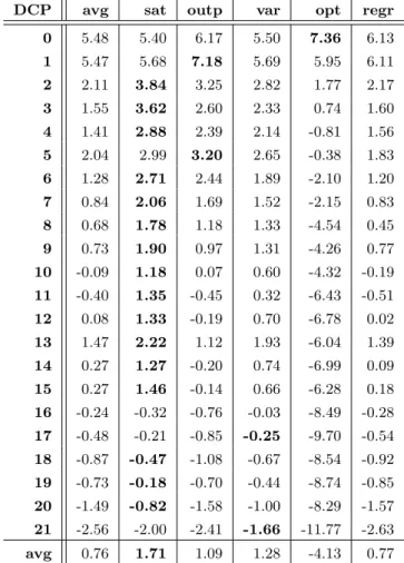
At LSB, data is collected and forecasts are calculated at 23 data collection points (DCPs) atwith fixed distances prior to the departure date of a flight. The number of days to departure assigned to each of the DCPs is shown in table 2.1. At each of these points, booking and cancellation numbers are recorded.
DCP 0 1 2 3 4 5 6 7 8 9 10 11
days to departure 350 182 140 126 98 70 56 49 42 35 28 21
DCP 12 13 14 15 16 17 18 19 20 21 22
days to departure 14 12 10 8 6 5 4 3 2 1 0
Table 2.1: Days to departure for each data collection point (DCP). Booking and cancellation data are furthermore collected for different dimensions:
• ODO - the origin-destination opportunity. One ODO holds past and present data of flights on the same routing with similar departure times, thus creating a stable history pool for a flight that is unaffected by flight number changes or minor time adjustments to the schedule.
• F - the fareclass (booking class). LSB distinguishes 20 fareclasses differing in price and booking conditions.
• DOW - the day of the week. Data is collected separately for each day of the week.
• POS - the point of sale. This indicates where a ticked was sold, it can be either the ’country of origin’, the ’country of destination’, or ’other’.
For capacity control, forecasts are generated on the finest possible level (for each ODO, F, DOW and POS combination), but are frequently aggregated to higher levels, for example for visualisation purposes or to support management decisions. The historical numbers for demand and cancellations are treated as univariate time series.
The airline industry environment comes with a few application-specific characte-ristics that have to be taken into account in the forecasting process: the fine level at which the forecasts are calculated causes a so called ‘small number problem’, which occurs due to the fact that for some combinations of ODO, F, DOW and POS, there might be only very few bookings, or no bookings at all. This means that small changes in the values lead to wide variances, so that the data is likely to be unstable and it becomes hard to build a model.
The fine level data is furthermore very noisy and susceptible to structural breaks, which are more or less abrupt changes in customer behaviour caused by seasonal ef-fects, events or other unforeseen circumstances. A constantly changing environment requires the forecasts to have adaptation capabilities. In many cases, choices made when building a model (for example parameter values, predictive model or aggre-gation level used) can lead to deteriorating performance as time passes and the decisions become suboptimal very quickly. In the live application, strong time re-strictions are another important factor, as a large number of forecasts needs to be generated in a limited amount of time.
This structure and quality of the existing data leads to the situation that in prac-tice, only a few methods could be identified to produce fairly accurate forecasts for the LSB application investigated here. A number of LSB internal and commissioned studies on this topic have shown that simple and robust time series forecasting mod-els such as simple average, different versions of exponential smoothing or regression models, which will be explained in more detail later, perform significantly better than a number of well known more sophisticated methods. This is not an obser-vation specific to LSB, as a survey involving several other industries performed by Jain (2008) reveals. In the survey, most of the participants report using either sim-ple trend/simsim-ple average models (57%) or models based on exponential smoothing (29%). The reason lies in the ability of the simple methods to make adequate fore-casts even on limited historical data by reducing the danger of overfitting on the training data, because the number of parameters to be estimated is small.
The next section describes algorithms currently used along with alternative ap-proaches implemented for the experiments presented at the end of this chapter. 2.1.4.2 Reference curves
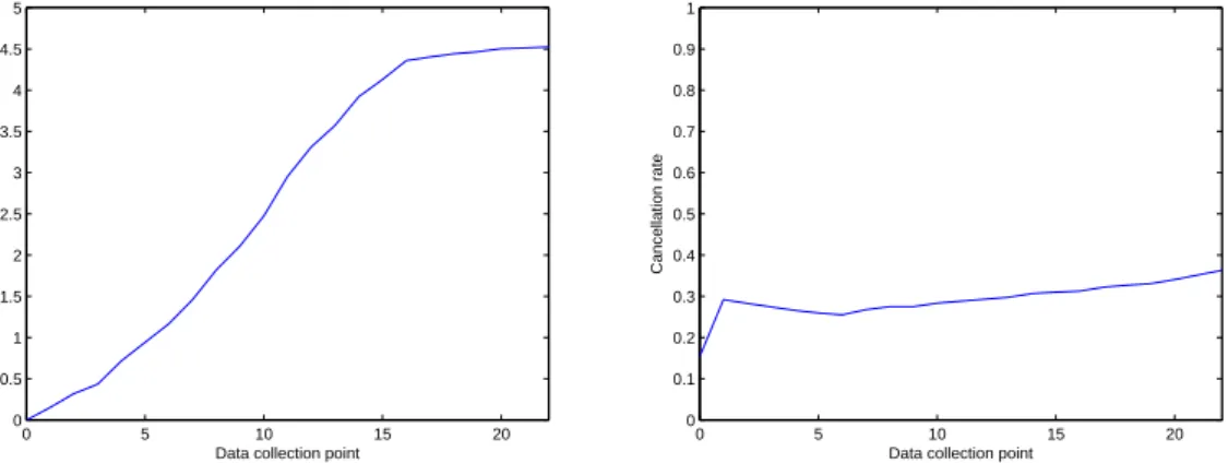
In general, forecasting at LSB makes use of reference curves for modelling the typical booking and cancellation behaviour of customers. They are learnt on the finest possible level for each DCP and are periodically updated with actual bookings and cancellation rates. Figure 2.2 shows examples of aggregated booking and cancellation reference curves. Cancellation information is usually represented as cancellation rates by dividing cancellation numbers by bookings.
0 5 10 15 20 0 0.5 1 1.5 2 2.5 3 3.5 4 4.5 5
Data collection point
Number of bookings 0 5 10 15 20 0 0.1 0.2 0.3 0.4 0.5 0.6 0.7 0.8 0.9 1
Data collection point
Cancellation rate
Figure 2.2: Example of reference curves, bookings (left) and cancellation rate (right), values given for each of the 23 DCPs prior to departure.
Reference curves are periodically updated in a history building step. If a new flight is introduced, an initial reference curve is generated using similar flights. The ba-sic calculation uses an exponential smoothing approach to calculate the new value refnew(dcp), taking into account both the previous value of the reference curve at the same DCP refold(dcp) and the current observation cr(dcp), weighted by a smoothing factor α, which controls how much the curve adapts to newly available data. This is described in Equation 2.1.
One of the problems arising in this context is the update of early parts of the cancellation rate reference curves, which only happens rarely: as long as booking numbers are zero and no rate can be obtained, the value of the old reference curve stays unchanged. To overcome this issue, changes in the reference curve at later data collections points are to a certain extent also used for updating the previous ones.
2.1.4.3 Unconstraining
As mentioned in the introduction, fareclasses are closed and opened during the op-timisation process. This influences booking numbers, as bookings are not registered for a closed fareclass even though the demand may exist. Accepted bookings and cancellations are thusconstrained, however, “unconstrained” numbers are needed for forecasting. Unconstraining is the process of eliminating the influence of capacity control from the data by approximating complete demand and cancellations. For bookings, unconstraining uses the reference curve in a simple additive manner to estimate demand that occurs during the time a fareclass is closed. For cancellations, a rate is calculated as a weighted sum of the actual cancellation rate applied to the actual bookings and the reference rate applied to the approximated rejected book-ings. Consequently, for fareclasses that have at some point been closed before flight departure, the data used for evaluation and forecasting purposes is not real data, but an approximation.
2.1.4.4 Booking forecast
The central question of booking forecasting is how many people would make a book-ing if it was accepted. An important concept for forecastbook-ing the bookbook-ing time series is decomposition. It is based on the assumption that time series are aggregates of a number of components, which can be modelled independently as separate time series. This approach is widely used in airline revenue management applications. In the most popular version, a time series is decomposed into a basic level, a trend and a seasonal component. The splitting of a series according to different factors allows separate treatment of each of the sub-series, with model and parameter choices being simpler and more adequate to the specific characteristics of a component.
At LSB, two major components are distinguished for bookings: theattractiveness
represents a stable base component, subject only to general long term influences like demographic and economic conditions or time slot of the flight. Other influences only have a short term effect, some of which cannot be predicted using historic data, for example if they occur due to special events like a football world champi-onship. However, other short term influences like seasonal behaviour can very well be modelled by examining the past. A previous project by Riedel (2007) provides a more detailed look at demand forecasting, with the focus on improving seasona-lity predictions as a big impact factor for final forecast accuracy. Overall accuracy improvements of 11% have been achieved.
2.1.5 Lufthansa Systems cancellation forecasting
Accurate cancellation predictions are vital for obtaining an accurate final net book-ing forecast, which is given by the difference of the bookbook-ing and cancellation fore-casts. In general, calculations concerning cancellations are carried out using can-cellation rates, i.e. the number of cancan-cellations divided by the number of bookings,
which has been shown to lead to more stable results in comparison to dealing with absolute cancellation numbers. This section first introduces the important concept of confidence limits for cancellation rates before moving on to the description of three traditional, rate-based algorithms.
2.1.5.1 Confidence limits
The small number issue described earlier introduces the problem of instability of cancellation rates. If, for example, only one booking exists in a specific fareclass, cancellation rates can be as extreme as zero or one, depending on whether or not the booking is cancelled. To prevent unstable cancellation rates especially at early data collection points where booking numbers are usually low, confidence limits1 are introduced and used to constrain the currently observed cancellation rate for both history building and forecasting to a certain range around the reference curve. Figure 2.3 shows the concept: an upper limit restricts cancellation rates that are much higher than the reference curve, a lower limit does the same for cancellation rates that are too low in comparison to the historically learnt behaviour. For the calculation, the following guidelines apply:
The confidence limits get wider (less restrictive) with
• an increasing number of bookings, as more bookings lead to a more stable cancellation rate,
• an increasing DCP, as data from DCPs closer to departure is more trustworthy and
• decreasing difference between expected bookings and already accepted book-ings. 0 5 10 15 20 0 0.1 0.2 0.3 0.4 0.5 0.6 0.7 0.8 0.9 1
Data collection point
Cancellation rate
reference curve confidence limits
Figure 2.3: Reference curve and confidence limits
2.1.5.2 Forecasting based on cancellation rate reference curves
Based on the current cancellation rate crt and reference curve reft,t being the time
index, two approaches exist for calculating the forecast. An additive approach is employed when
1Confidence limits are not to be confused with confidence intervals, which have a completely
• crt<reftand reft is ascending or
• crt>reftand reft is descending
and a multiplicative approach is used in case
• crt>reftand reft is ascending or
• crt<reftand reft is descending.
The additive approach following Equation 2.2 enforces a bigger adjustment by just adding or subtracting the appropriate values of the reference curve, while the multi-plicative approach ensures that the results are not below zero or above one by more gentle adjustments given in Equations 2.3 and 2.4, with indext+hbeing the current timet plus the forecasting horizonh.
ˆ crt+h = crt+ (reft+h−reft) (2.2) ˆ crt+h = 1− 1−reft+h 1−reft ·(1−crt) for crt>reft (2.3) ˆ crt+h = reft+h reft ·crt for crt<reft (2.4)
Default cancellation rates that are used to initialise reference curves are generated from similar flights and have been provided by LSB. Three ways of updating them are currently implemented:
• A model based on single exponential smoothing, where a new forecast is gene-rated by adjusting the previous one by the error it produced. Reference curves are updated using Equation 2.1.
• A model based on Brown’s double exponential smoothing according to Brown et al. (1961). The updated value reft is calculated using the equations below,
with L being the value (level) of the series, T the trend component and α
again the constant smoothing factor. reft = Lt+Tt
Lt = α·crt+ (1−α)·(Lt−1+Tt−1) (2.5)
Tt = α·(Lt−Lt−1) + (1−α)·(Tt−1)
• A regression model that uses a regression line fitted to past observations of the same DCP. The new value for the reference curve is calculated by extrapolating the regression line into the future, a value for the trend curve is obtained from its slope.
Similar to the current algorithm used for the booking forecast, the current cancella-tion forecast is a mixture of some of these algorithms, with details being confidential. The forecasts of the currently used method will however be used as a baseline for comparison in the empirical experiments and will furthermore be referred to as the LSB cancellation forecast.
2.1.5.3 Probability forecast
In meetings with LSB, it was brought up that another cancellation forecast based on probabilities might be able to produce accurate results while still being simple and robust. As a reaction, a fourth forecast has been implemented in the scope of this work to add a functionally different approach to the method pool. The central question here is: for a booking at a certain DCP, what is the probability that the booking is cancelled at following DCPs if it has not been cancelled before?
The algorithm is based on the assumption that bookings occurring at different DCPs will have different probabilities of being cancelled prior to departure of the flight. It was, for example, previously observed, that bookings from early DCPs tend to be cancelled more often than the bookings from later ones. Similarly to the previously introduced approaches, reference curves are generated in the history building step. In the probability reference curve, each booking is assigned to a DCP, and the probability that it will be cancelled on a later DCP is given. A simplified example in form of a table is shown in Table 2.2. It says, for example, that a booking made at DCP0 will be cancelled at DCP1 with a probability of 0.15, if it has not been cancelled before. A booking from DCP2 obviously does not have probabilities for cancellation at DCP0 and 1, as it only occurred at a later DCP.
P(Canc. at DCP0) P(Canc. at DCP1) P(Canc. at DCP2)
Booking at DCP0 0.1 0.15 0.1
Booking at DCP1 - 0.2 0.1
Booking at DCP2 - - 0.15
Table 2.2: Simplified example of a cancellation probability reference curve. Apart from a few special cases where booking numbers are extremely small, it is not possible to tell which occurring cancellation belongs to which booking. This is why the previously generated probabilitiesP(j, t), giving the probability that a booking from DCPj will be cancelled at DCP t,j ≤t, are used to distribute cancellations to previous bookings as demonstrated in Equations 2.6 and 2.7. Assume a number of cancellationsct occur at DCPt. All remaining bookingsbi at the previous DCPs
0 ≤ i ≤ t are then adjusted according to Equation 2.6 in case that the number of cancellations is greater than the sum of the product of relevant bookings and probabilities (Pt
j=0bjPj,t > ct) and according to Equation 2.7 otherwise.
bnewi = bi−λ(bi·Pi,t), λ= ct Pt j=0bjPj,t (2.6) bnewi = bi−bi(1−λ(1−Pi,t)), λ= Pt j=0bj −ct Pt j=0bj(1−Pj,t) (2.7) The cancellation probability that is eventually used for updating the probability reference curves is then obtained by dividing the new value of remaining bookings
bnewi by the old valuebiand subtracting it from 1. Initial probability reference curves
are generated in a history building period, where cancellations are evenly distributed on previous bookings.
The forecasting process then consists of two steps: for each DCP, the current cancellations are first distributed to past bookings with the same algorithms as
used in the history building. Secondly, the booking reference curve estimates the development of the bookings for the future DCPs. Applying the probabilities from the reference curves and summing up the remaining bookings creates the final net booking forecast.
In summary, it can be said that demand and cancellation forecasting methods used at LSB have been heavily tuned to account for application-specific characteris-tics and requirements. The basis of the presented algorithms are simple averages and exponential smoothing approaches. However, many more methods have been inves-tigated in the scientific literature, which will be reviewed in the remaining sections of this chapter.
2.2 Time series forecasting
This section looks at forecasting from a more general point of view and investigates traditional time series forecasting to provide the basis for the remainder of the thesis, aiming at organising and highlighting the most important methods and results of half a century’s research done in this area.
The most basic time series forecasting method is called the naive forecast and sets the forecast to the last time series observation. Another simple method is the moving average, where the forecast is the arithmetic mean of the most recent values of the time series, discarding old and potentially inapplicable observations. Beyond these, the first more sophisticated methods date back to the 1950’s and 1960’s, with new approaches and extensions constantly being investigated until today. This sec-tion provides a literature review of the most important and popular approaches to time series forecasting. The choice of publications to cite has been difficult, as a vast majority of contributions are smaller case studies applied to a specific appli-cation area, which mostly provide results that contradict each other. As individual forecasting algorithms are not the primary focus of this thesis, the literature review will be confined to five big groups of forecasting algorithms, discussing the seminal contributions, publications on genuinely new forecasting algorithms and extensive review papers. Only a selection of the approaches mentioned here are actually im-plemented for the empirical studies in this thesis, which is why equations and more detailed descriptions of only these will be given along with the methodology of the experiments in Section 3.2.2.
2.2.1 Exponential smoothing
Exponential smoothing methods apply weights that decay exponentially with time and thus also rely on the assumption that more recent observations are likely to be more important for a forecast than those lying further in the past. Smoothing methods originated in the 1950’s and 1960’s, with the methods of Brown, Holt and Winter still being of considerable importance today as summarised and referenced in Makridakis et al. (1998). The seemingly only originally new smoothing method since the classic approaches was introduced by Taylor (2003), who suggested using a damped multiplicative trend; details are given in Section 3.2.2.1. A taxonomy of exponential smoothing methods has first been presented by Pegels (1969), distin-guishing between nine models with different seasonal effects and trends, which can be additive, multiplicative or non-existent. Gardner (1985) extended this classification by including damped trends, increasing the number of models to twelve.
Abraham & Ledolter (1986) showed that some exponential smoothing methods arise as special cases of ARIMA models. Apart from this, these methods have been lacking a sound statistical foundation for a long time, which prevented a uniform approach to calculation of prediction intervals, likelihood and model selection cri-teria. Hence, many publications were concerned with investigating the stochastical framework of the exponential smoothing methods. The most thorough and recent work in this context has been published by Hyndman et al. (2002), who fitted all of the twelve models of Gardner (1985) into a state space framework, giving state space equations for each of them using both an additive and a multiplicative error approach. They furthermore fit a model selection strategy to the framework in order to allow for automatic forecasting.
A recent variation drawing some attention is the Theta-model proposed by As-simakopoulos & Nikolopoulos (2000). It decomposes seasonally adjusted series into short and long term components by applying a coefficient θ to the second order differences of the time series, thus modifying its curvature as described in Section 3.2.2.1. Hyndman & Billah (2003) show that this method is equivalent to single exponential smoothing with drift.
Extensive state-of-the art reports on exponential smoothing can be found in Gardner (1985) and Gardner (2006), citing over 100 and 200 relevant papers, re-spectively.
Exponential smoothing methods have a reputation of performing remarkably well for their simplicity as summarised in Gooijer & Hyndman (2006). In an exten-sive competition conducted by Makridakis & Hibon (2000), the authors recommend Taylor’s exponential smoothing method with dampened trend as a method that is very easy to implement and gives robust performance. Chatfield et al. (2001) ar-gue that the robust nature of these models is due to the fact that they are the best choice for a large class of problems. Hyndman (2001) picks up on that and adds that more complex models are subject to performance instabilities caused by a more complex model selection and parameter estimation process, which exponential smoothing models do not suffer from to this extent.
2.2.2 ARIMA models
One of the most influential publications in the area of time series forecasting is Box & Jenkins (1970), having an extraordinary impact on forecasting theory and practice until today. The authors introduced the group of autoregressive integrated moving average (ARIMA) models, which can simulate the behaviour of diverse types of time series. An ARIMA model consists of an autoregressive and a moving average part whose orders have to be estimated and involves a certain degree of differencing; general equations are given in Section 3.2.2.2.
Selection of an appropriate model can be done judgementally. A strategy mainly based on examining (partial) autocorrelation values can be found in Makridakis et al. (1998). Alternatives have been suggested, for example using information criteria like Akaike’s information criterion (AIC)2 introduced in Akaike (1973) and Bayes information criterion (BIC)3 introduced in Raftery (1986). More recent publications mostly apply ARIMA models in a hybrid approach, for example in combination
2AIC= 2k−2·ln(L), withkbeing the number of parameters in the model andLthe maximized
value of the likelihood function for the estimated model. 3
BIC =−2·ln(L) +k·ln(n), wherek andL are the same as for the AIC andn denotes the
with neural networks as in Zhang (2004) and Koutroumanidis et al. (2009) or as an individual method as part of a more general combination approach as in Anastasakis & Mort (2009).
The performance and benefits of ARIMA models has been fiercely discussed in the aftermath of the M3-competition, whose results have been published in Makri-dakis & Hibon (2000). In this publication, the organisers criticise the approach of building statistically complex models like the ARIMA model, disregarding all empi-rical evidence that simpler ones predict the future just as well or even better in real life situations, for example provided by their competition. Makridakis et al. (1998) furthermore add that the only advantage a sophisticated model has compared to a simple one is the ability to better fit historical data, which is no guarantee for a better out-of-sample performance. Results of the M3 competition are discussed from a more general point of view in the next chapter.
2.2.3 State-space models
State space models provide a framework that can accommodate any linear time series model. The seminal work in this area was published by Kalman (1960), giving a recursive procedure for computing forecasts known as the Kalman filter. Originally mainly used in control and engineering applications, its usage for time series forecasting only started in the 1980’s according to Gooijer & Hyndman (2006). Generally, two equations are part of a state space model: the observation and the state equation. While the state equation models the dependency of the current to the previous state, the observation equation provides the observed variables as a function of the state variables. A state-space model was implemented for the empirical experiments of this thesis as described in Section 3.2.2.3.
Gooijer & Hyndman (2006) mention that publications from practitioners con-cerning the use of the state space framework for time series forecasting applications are surprisingly rare, even though some books do exist, for example Durbin & Koop-man (2001). Two significant contributions can however be mentioned: Harvey (2006) provides a comprehensive review and introduction to treating “structural models”, i.e. time series given in terms of components such as trends and season, with the help of the state space concept. As already cited above, Hyndman et al. (2002) fit exponential smoothing methods into state space framework, providing them with a statistical foundation.
Comparing the performance of state-space models is not straightforward by look-ing at available literature, as they do not seem to appear in the major forecastlook-ing competitions. Since a large number of models have state-space formulations, the performance will naturally vary according to the model used. However, the benefits related to their statistical theory, e.g. well-defined strategies for model selection, likelihood estimation and prediction interval calculation are bound to make them attractive for forecasting researchers and practitioners.
2.2.4 Regime switching
Regime switching models are a class of model-driven forecasting methods originally introduced by Tong (1990). Most of them belong to the class of so-called self-exciting threshold autoregressive models (SETAR) and their variants, where a number of regimes consists of one autoregressive model each. The order and coefficients of the autoregressions vary for each regime. Which set of equations to apply for a
forecasting situation is then determined by trying to identify the regime or state the system is likely to be in, which is normally done by looking at past values of the time series, hence the term “self-exciting”. Some SETAR models have been compared in Clements & Smith (1997).
As abruptly changing regimes are not always desirable, smooth switching of regimes is promoted in smooth transition autoregressive (STAR) models, where switching can, for example, be done with a logistic function. A publication by van Dijk & Franses (2000) gives a survey of developments in this area at this time. More recent work was published in Fok et al. (2005), where a STAR model is complemented with a meta-model linking parameters of the logistic switching functions to state characteristics and other regressors.
Empirical evaluation of regime switching models has mainly been conducted in comparison to neural networks and linear models and produced mixed results. In Stock & Watson (2001), STAR models generally performed worse than neural networks and did not outperform linear models either. Ter¨asvirta et al. (2004) however question results of this study, stating that nonlinear forecasting methods should only be considered at all if the data shows nonlinear characteristics. A re-examination of the performances of linear, STAR and neural network appr