Improving the performance of causality analysis techniques for automated fault diagnosis in mineral processing plants

(1)

Brian Siegfried Lindner

Dissertation presented for the degree of

Doctor of Philosophy (Extractive Metallurgical Engineering)

in the Faculty of Engineering at Stellenbosch University

Supervisor: Dr. Lidia Auret

(2)

Declaration

By submitting this dissertation electronically, I declare that the entirety of the work contained therein is my own, original work, that I am the sole author thereof (save to the extent explicitly otherwise stated), that reproduction and publication thereof by Stellenbosch University will not infringe any third party rights and that I have not previously in its entirety or in part submitted it for obtaining any qualification.

Date: April 2019

(3)

(4)

Plagiarism declaration

1. Plagiarism is the use of ideas, material and other intellectual property of anothers work and to present is as my own.

2. I agree that plagiarism is a punishable offence because it constitutes theft. 3. I also understand that direct translations are plagiarism.

4. Accordingly all quotations and contributions from any source whatsoever (including the in-ternet) have been cited fully. I understand that the reproduction of text without quotation marks (even when the source is cited) is plagiarism.

5. I declare that the work contained in this dissertation, except where otherwise stated, is my original work and that I have not previously (in its entirety or in part) submitted it for grading in this dissertation or another document.

Initialsand surname: B.S.Lindner Date: April 2019

(5)

(6)

Abstract

Modern mineral processing companies are driven towards improving productivity by leveraging existing processes optimally. This can be achieved by improving diagnosis of faults that degrade process performance to provide insightful and actionable information to process engineers. In mineral processing plants, units and variables are connected to each other through material flow, energy flow, and information flow. Faults propagate through a process along these intercon-nections, and can be traced back along their propagation paths to their root causes. Techniques have been developed for extracting these causal connections from historical process data. These techniques have proven successful for fault diagnosis in chemical processes. However, they have not been widely accepted by industry due to lack of automation of the techniques, complicated implementation, and complicated interpretation.

This dissertation investigated the limitations of the causality analysis procedures currently avail-able to process engineers as fault diagnosis tools and developed improvements on them. Improve-ments were developed and tested using a combination of simulated case studies and real world case studies of operational faults occurring in a mineral processing plant.

Objective I: was to investigate the factors that affect performance of causality analysis tech-niques. The use of transfer entropy for fault diagnosis in a minerals processing concentrator plant was demonstrated. The desired performance criteria of causality analysis techniques were then defined in terms of: general applicability; automatability; interpretability; accuracy; precision; and computational complexity. The impact of process conditions on the performance of Granger causality and transfer entropy were then investigated. An analysis of variance (ANOVA) was performed to investigate the impact of process dynamics, fault dynamics, and the parameters on the accuracy of transfer entropy.

Objective II:was todesign a systematic workflow for application of causality analysis for fault diagnosis. The ANOVA was used to develop a novel relationship between the optimal transfer entropy parameters and the process and fault dynamics. This relationship was then placed within a systematic workflow developed for the application of transfer entropy for oscillation diagnosis, addressing the need for clear procedures and guidelines for data selection and param-eter selection. The workflow was applied to an oscillation diagnosis case study from a minerals concentrator plant, and shown to provide a systematic approach to accurately determining the fault propagation path.

Objective III: was to design a tool to aid the decision of which causality analysis method to select. A comparative analysis of Granger causality and transfer entropy for fault diagnosis based on the performance criteria defined was performed. The comparison showed that transfer entropy was more precise, generalisable, and visually interpretable. Granger causality was more automatable, less computationally expensive, and easier to interpret. Guidelines were developed from these comparisons to aid users in deciding when to use Granger causality or transfer entropy.

(7)

Objective IV: was to present tools for interpretation of causal maps for root cause analysis. Methods for construction of causal maps from the results of the causality analysis calculation were presented, and methods for interpretation of causal maps. The usefulness of these tech-niques for diagnosis of real world case studies was demonstrated.

(8)

Uittreksel

Mineraalprosesseringsmaatskappye plaas hul fokus op die verhoging van produktiwiteit deur bestaande prosesse te optimeer. Dit word bereik deur op ‘n meer doeltreffende manier foute op te spoor wat prosesprestasie hinder en sodanig insiggewende inligting aan prosesingenieurs oor te dra.

Proseseenhede en veranderlikes word verbind aan mekaar in ‘n mineraalproseseringsaanleg deur die vloei van material, energie en inligting. Foute word deur ‘n proses voortgesit deur die verbintenis van die proseseenhede aan mekaar, en die kernoorsaak van ‘n fout kan opgespoor word deur terug te werk deur prosesverbintenisse. Tegnieke is ontwikkel om oorsaaklike verbintenisse te onttrek vanuit historiese prosesdata. Hierdie tegnieke word as suksesvol geag vir foutdiagnose in chemiese prosesse. Hulle is egter nie in die mineraalprosesseringsbedryf aanvaar nie weens die tekort aan die moontlikheid van outomasie, die ingewikkelde implementasie daarvan, asook ingewikkelde interpretasie.

Hierdie verhandeling ondersoek die beperkinge van beskikbare oorsaaklikheidsanalisemetodes as foutdiagnosegereedskap vir prosesingenieurs en ontwikkel verbeteringe op die metodes. Verbe-terings is ontwikkel en getoets deur ‘n kombinasie van gesimuleerde gevallestudies en werklike gevallestudies van ‘n mineraalprosesseringsaanleg.

Doel I:was om faktore teondersoek wat die prestasie van oorsaaklikheidsanalises affekteer. Die gebruik van oordragsentropie vir foutdiagnose in ‘n mineraalprosesserings konsentrasie-eenheid is gedemonstreer. Die gewenste prestasiekriteria van oorsaaklikheidsanalises is toe gedefinieer in terme van: algemene toepaslikheid; outomiseerheid; interpreteerbaarheid; akkuraatheid; pre-sisie; en berekeningkompleksiteit. Die impak van prosestoestande op die prestasie van Granger oorsaaklikheid en oordragsentropie is toe ondersoek. ‘n ANOVA variansieanalise is toe uit-gevoer om die impak van prosesdinamika, foutdinamika, en geselekteerde parameters op die akkuraatheid van oordragsentropie te ondersoek.

Doel II: was om ‘n systematiese werksvloei te ontwerp vir die toepassing van oorsaaklikheid-sanalises op foutdiagnose. Die ANOVA was gebruik om ‘n nuwe verhouding te ontwikkel tussen die optimale oordragsentropieparameters en die proses- en foutdinamika. Hierdie verhouding is toe in ‘n sistematiese werksvloei geplaas ontwikkel vir die toepassing van oordragsentropie vir ossillasiediagnose, wat die nodigheid vir duidelike prosedures en riglyne vir data- en parame-terseleksie addresseer het. Die werkvloei is toegepas op ‘n ossilasiediagnose gevallestudie van ‘n mineralekonsentrasieaanleg, en is gewys om ‘n systematiese benadering te verskaf om die foutvoortplantingspad akkuraat vas te stel.

Doel III: was om gereedskap te ontwerp om te help besluit tussen oorsaaklikheidsanaliseme-todes. ‘n Vergelykende analise van Granger oorsaaklikheid en oordragsentropie vir foutdiag-nose gebaseer op gedefinieerde prestasiekriteria is uitgevoer. Die vergelyking het getoon dat oordragsentropie meer presies, veralgemeenbaar en visueel interpreteerbaar is. Granger

(9)

saaklikheid is meer outomeerbaar, minder berekeningsintensief en makliker om te interpreteer. Riglyne is ontwikkel vanuit hierdie vergelykings om verbruikers te help kies tussen Granger oorsaaklikheid en oordragsentropie.

Doel IV: was om gereedskap voor te stel vir die interpretasie van oorsaaklikheidskaarte vir kernoorsaakanalises. Metodes om oorsaaklikheidskaarte op te stel vanuit die resultate van oor-saaklikheidsanaliseberekeninge is voorgestel, asook metodes vir die interpretasie van oorsaak-likheidskaarte. Die nut van hierdie tegnieke vir die diagnosering van werklike gevallestudies is gedemonstreer.

(10)

Acknowledgements

The author wishes to acknowledge the following people and institutions for their various contributions towards the completion of this work:

• The supervisors of this project, Dr. Lidia Auret and Prof. Margret Bauer, for their support, guidance, feedback, and advice for this project.

• Anglo American Platinum Limited, for their extensive support of this project. This sup-port included funding, access to data, and access to process expertise from process engi-neers.

• Dr. J.W.D Groenewald at Anglo American Platinum Limited, for support and guidance during this project, for contributing useful industrial perspective to the project, and for contributing as co-author on two of the papers published on this research.

• ABB Corporate Research Centre in Ladenburg, Germany, for facilitating a research ex-change visit.

• Dr. Moncef Chioua at ABB Corporate Research in Ladenburg, Germany, for his useful guidance and insights for this project, and for contributing as co-author on one of the papers published on this research.

• Stone Three Digital, and my colleagues there for support during my project, and for allowing me the freedom to complete the project part time.

• My girlfriend, Patsy, for her continuous support during this project. • My family for support and encouragement during this project.

(11)

(12)

Glossary

Adjacency matrix Matrix representation of a graph. Square matrix whose rows and columns correspond to nodes, and binary entries represent the edges.

Causality Links between elements in a process, so that a change in one element cause a change in another, and the direction of the influence is known.

Causality map Graph with nodes representing measured variables, and edges representing causal connections between them.

Connectivity Links between elements in a process, so that changes in either variable influence the other.

Cross correlation Causality measure base on lagging two time series to find the time lag at which the correlation between them is at a maximum

Convergent cross-mapping Causality measure based on the mutual prediction ability of em-bedding manifolds

Depth-first search Algorithm for graph traversal. Works by beginning at a start node, and discovering adjacent nodes sequentially until the algorithm encounters a node where all the adjacent nodes have already been visited. At this point, the search backtracks along the discovered path to the closest previously discovered node without a discovered neighbour. This is implemented recursively until all nodes reachable from the start node have been visited.

Diffeomorphism Isormorphism of smooth manifolds.

Edge Connection between nodes in a graph. Also called arc In causality maps it indicates a causal connection between two measured variables.

Fault Abnormal event occurring in a process that causes measured variables or KPIs to deviate from desired values, possibly causing performance or safety degradation.

Fault detection Procedure for determining whether a fault is present in a process or not.

Fault diagnosis Combination of fault detection and identification.

Fault identification Procedure for determining the type, magnitude and location of a fault.

Granger causality Causality measure based on autoregressive models. Quantifies the predic-tion improvement of a variable when including past values of another variable.

Graph A mathematical model of pairwise relationships between elements. Consists of nodes representing the elements, and edges representing the relationship between the elements.

(19)

Hazard and operability analysis Risk analysis performed typically during process design phase to identify all potential safety and performance degradation risks.

Inflow Number of edges entering a node.

Isomorphism Mapping that can be reversed using the inverse of the mapping.

k-Nearest Neighbours In this dissertation this refers to a causality measure based on predic-tion of a variable based on its nearest neighbours.

Node Element in a graph. Also called vertex. In a causality map it represents measured variables.

Outflow Number of edges exiting a node.

Partial directed coherence Causality measure based on frequency-domain autoregressive mod-els.

Process monitoring Strategy for analysing process behaviour to determine performance.

Process recovery Corrective action taken to return a process to its desired state after devia-tion from this state has been diagnosed.

Process topology The way in which constituent parts of the model are interconnected. May be described in terms of connectivity or causality of the variables in the process.

Reachability Ability to negotiate from one node to another within a graph

Root cause analysis Procedure for isolating the location of a fault.

Smearing effect The effect of a fault spreading throughout a process and affecting numerous variables and units.

Strongly connected component A subgraph of of a graph, G, where all the nodes in the subgraph are mutually reachable.

Subgraph A subgraph of a graph,G, is a graph made of a subset of the nodes and edges ofG.

Transfer entropy Information theoretic causality analysis approach. Quantifies the reduction in uncertainty of one variable given past values of another variable.

Transitive reduction The transitive reduction of a graph G, is another graph, Greduction,

with the same number of nodes, but the fewest edges, so that Greduction has the same

reachability as G.

(20)

List of Reserved Symbols

Symbols in this dissertation conform to the following font conventions:

A Symbol denoting a variable (Upper case letter)

a symbol denoting a scalar (Lower case letter)

a Symbol denoting a vector (Bold lower case letter)

A Symbol denoting a matrix (Bold upper case letter)

Symbol Meaning

αk Random phases added for AAFT

A Coefficient matrix for full AR model

B Regression coefficient for reduced AR model

Di(x) Predictability factor for k-nearest neighbours di,j Distance between two embedded vectors,iand j

E Prediction error matrix for autoregressive model

Prediction error in autoregressive model

Fxi→xj Granger causality from variablexi to variablexj

H(yi+h|yi(K)) Shannon entropy for y conditioned on past values of itself H(yi+h|y_i(K),x(_iL)) Shannon entropy for y conditioned on past values of xand y h Prediction horizon for transfer entropy

η(x|y) Dependence measure for k-nearest neighbours

ηx→y Causality measure for k-nearest neighbours

ι Imaginary unit

K Embedding dimension for output variableY in transfer entropy calculation

k Model order for Granger causality calculation

κ Number of nearest neighbours

L Embedding dimension for input variableX in transfer entropy calculation

M Number of variables

M Embedded matrix (manifold)

µ Mean

NS Number of samples

p(.) Probability density function

p(.|.) Conditional probability density function ˆ

πij(ω) partial directed coherence between variablei and variablej, at frequency, ω

ρ Cross-correlation function

¯

r(t) iAAFT surrogate time series ¯

R(ω) Frequency domain representation of ¯r(t)

σ Standard deviation

¯

s(t) AAFT surrogate time series

Sx→y Significance threshold for transfer entropy fromx toy

(21)

TS Sampling time

Tx→y Transfer entropy from variablex to variabley τ Time interval for transfer entropy

τp Residence time of process

x(_iL) Embedded vector for variablex, at time step i, with embedding dimension, L yi+h Value of variabley at time step i+h

(22)

List of Abbreviations

AAFT: Amplitude Adjusted Fourier Transform

AIC: Akaike Information Criterion

AML: Automation Markup Language

APC: Advanced Process Control

ANOVA: ANalysis Of VAriance

AR: AutoRegressive

CCM: Convergent Cross Mapping

CSTR: Continuous Stirred Tank Reactor

CV: Controlled Variable

DTE: Direct Transfer Entropy

DTF: Directed Transfer Function

FFT: Fast Fourier Transform

HAZOP: HAZard and OPerability

iAAFT: iterative Amplitude Adjusted Fourier Transform

KPI: Key Performance Indicator

KDE: Kernel Density Estimation

LSD: Least Significant Difference

MV: Manipulated Variable

NOC: Normal Operating Conditions

PCA: Principal Component Analysis

PDC: Partial Directed Coherence

PDF: Probability Density Function

PID: Proportional Integral Derivative

P&ID: Piping & Instrumentation Diagram

(23)

PGM: Platinum Group Metal

PV: Process Variable

RCA: Root Cause Analysis

SDG: Signed DiGraph

SDNTE: Symbolic Dynamic-based Normalised Transfer Entropy

SCC: Strongly Connected Component

VAR: Vector AutoRegressive

XML: eXtensible Markup Language

(24)

List of Figures

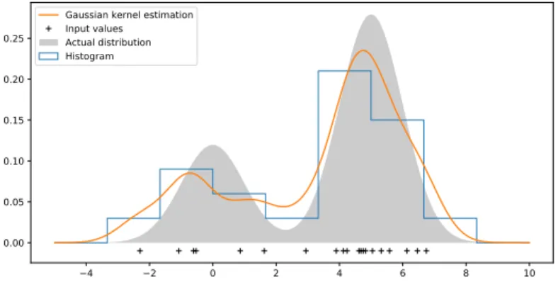
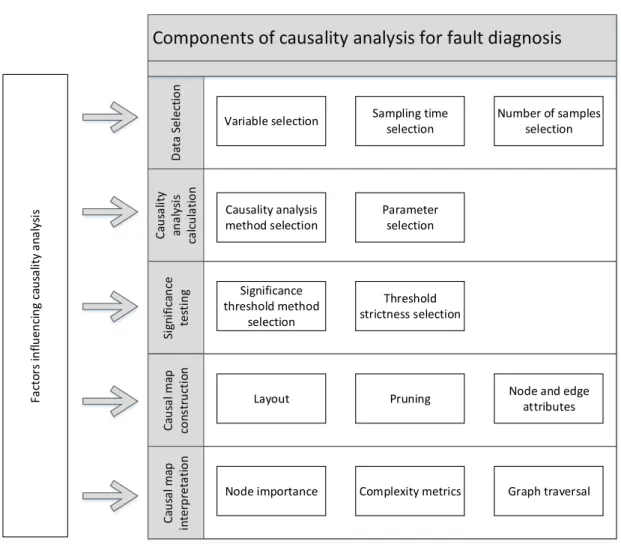
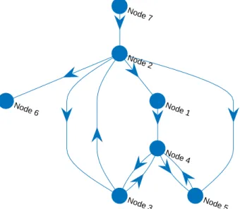
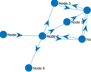
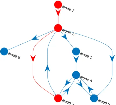
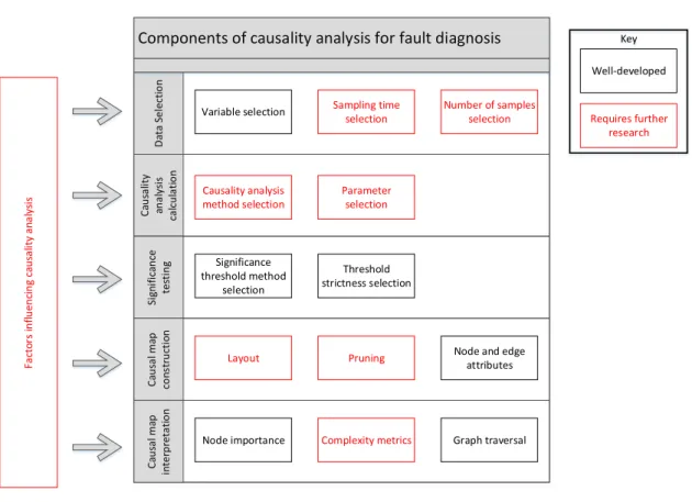
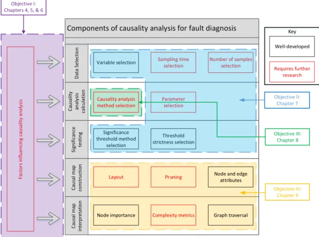
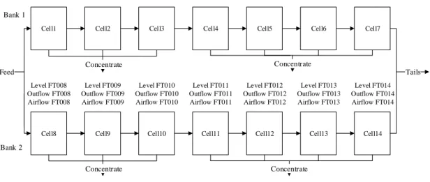
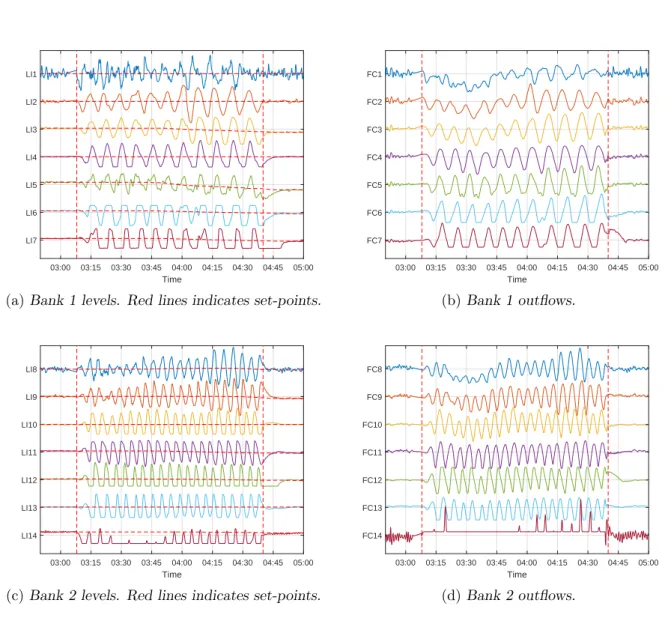
2.1 Process monitoring overview . . . 7 2.2 Simple causal map example . . . 9 2.3 Process monitoring loop . . . 13 2.4 Causal map with indirect connections . . . 22 2.5 Density estimation comparisons . . . 24 2.6 Gaussian kernel density estimation example . . . 25 2.7 Literature summary by industry . . . 34 2.8 Literature summary by method . . . 35 2.9 Overview of components of causality analysis . . . 36 2.10 Example of layered layout of causality maps . . . 45 2.11 Example of circle layout of causality maps . . . 46 2.12 Example of force layout of causality maps . . . 46 2.13 Causal map with indirect connections . . . 47 2.14 Transitive reduction illustration . . . 48 2.15 Transitive reduction illustration with cycles . . . 49 2.16 Straightforward causality map example . . . 49 2.17 Causality map demonstrating maximum flow attriute . . . 49 2.18 Example of shortest path found betweenN ode7 and N ode3 . . . 51 2.19 Overview of chapters addressing components of causality analysis . . . 52 3.1 Overview of chapters addressing components of causality analysis . . . 56 4.1 Transfer entropy basic methodology . . . 60 4.2 Causal map example . . . 61 4.3 Flotation circuit flow diagram . . . 62 4.4 Flotation case study oscillatory time series . . . 63 4.5 Flotation case study transfer entropy propagation paths . . . 65 4.6 Cyclone pressure disturbance . . . 68

(25)

5.1 Example of a cyclical graph . . . 75 5.2 Illustration of sensor and process noise . . . 76 5.3 Causal map for control loop . . . 77 5.4 Causal map with confounding connections . . . 78 5.5 Time frame for Granger causality and transfer entropy . . . 80 6.1 Diagram of simulated tank with heat exchange system . . . 82 6.2 Response of T1 to perturbations T1in. . . 84

6.3 Expected response of causality measures to perturbations . . . 85 6.4 Impact of oscillatory perturbations on Granger Causality and transfer entropy . 88 6.5 Impact of step perturbations on Granger causality and transfer entropy . . . 90 7.1 Workflow for application of transfer entropy for oscillation diagnosis . . . 94 7.2 Transfer entropy response to number of samples . . . 98 7.3 Transfer entropy response to sampling time . . . 99 7.4 Transfer entropy response to process dynamics . . . 100 7.5 Linear relationship between optimal time interval (τmax) and oscillation period (P)101

7.6 Linear relationship between oscillation period (P) and time delay (TD), and

op-timal time interval (τmax) . . . 102

7.7 Linear relationship between P and distance between τ peaks . . . 102 7.8 Flotation circuit flow diagram . . . 103 7.9 Flotation circuuit oscillatory time series . . . 104 7.10 Power spectra showing oscillation frequency . . . 105 7.11 Flotation case study transfer entropy parametrisation propagation path . . . 108 7.12 Flotation case study cyclone pressure . . . 109 8.1 Computational time required to calculate transfer entropy significance for one

pair of variables as a function of number of samples. System used: 32 GB RAM, 3.33 GHz processor. The computational time was found to be well approximated by CP Utime= 34×N0.5 . . . 116

8.2 Diagram of simulated two tank process. Two tanks in series with heat exchangers. Tank levels are controller by the flow of cold water into the tank, tank temper-atures are controlled by the steam flow rate through the heating coils. Random noise was added to the signals. . . 119 8.3 Oscillations in signals in two tank process. . . 120 8.4 Distributions of true connection rates and relative true connection rates for Granger

causality and transfer entropy in the simulated two-tank process. . . 120 8.5 Granger causality and transfer entropy results from repeated simulated

experi-ments compared to true propagation path. Results shown from minimum, median, and maximum true connection rates. . . 121

(26)

8.6 Decision flow for application of Granger causality or transfer entropy for fault diagnosis. . . 123 8.7 Simplified process flow diagram showing the primary milling circuit, the rougher

flotation section and the secondary milling section. . . 125 8.8 Trends for all variables showing oscillation at period of 69 minutes. This includes

variables from primary milling circuit, rougher flotation circuit, and secondary milling circuit. . . 126 8.9 Transfer entropy propagation paths for oscillations in the primary milling,

flota-tion, and secondary milling circuits. Values displayed on edges and edge width represent the transfer entropy value calculated. Colours on nodes indicated the section of the plant where the variables are located. . . 127 8.10 Time series plots of sump variables at start of oscillation. . . 128 8.11 Granger causality propagation paths for oscillations in the primary milling,

flota-tion, and secondary milling circuits. . . 129 9.1 Different layours for causality maps . . . 136 9.2 Transitive reduction for the primary milling oscillation . . . 138 9.3 Causality map for plant wide oscillation visualising connection strength using

edge width . . . 139 9.4 Causality map for both banks in flotation circuit . . . 141 9.5 Propagation paths for oscillations in the flotation circuit . . . 142 9.6 Causality map coloured according to plant sections . . . 143 9.7 Flotation circuit oscillations treating CVs and MVs separately . . . 145 9.8 Causality map for primary mill oscillation with maxflow highlighted . . . 146 9.9 Shortest path from SU1LevelP V toSU5Density. . . 148 9.10 All nodes reachable fromSU1LevelP V, found using the depth-first search . . . . 149 9.11 Procedure for interpretation of causal maps for fault diagnosis . . . 150 10.1 Overview of chapters addressing components of causality analysis . . . 154 A.1 ANOVA results for different levels of each factor . . . 169

(27)

(28)

List of Tables

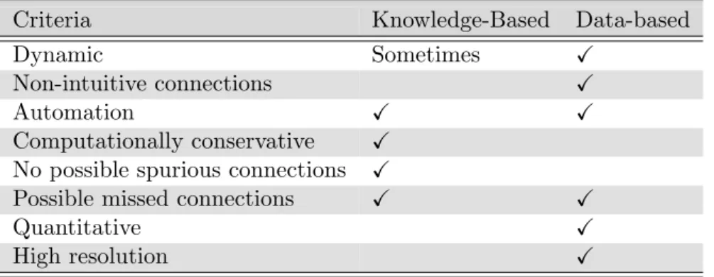
2.1 Comparing characteristics of knowledge and data-based causality . . . 31 2.2 Causality analysis literature summary . . . 31 2.2 Causality analysis literature summary . . . 32 2.2 Causality analysis literature summary . . . 33 2.3 Summary of decisions and parameter selection methods used for transfer entropy

in literature . . . 39 4.1 Flotation case study nonlinearity index results . . . 67 4.2 Flotation case study oscillation start times . . . 67 6.1 Tank simulation model parameters . . . 83 6.3 Ranges of perturbations used for sensitivity analysis . . . 84 6.4 Means and standard deviations of Granger causality and transfer entropies shown

in Figure 6.4. . . 86 7.1 Guidelines for transfer entropy parametrisation . . . 101 7.3 Time delay between level variables . . . 106 7.4 Time delay between outflow variables . . . 106 7.5 τ between level variables . . . 107 7.6 τ between outflow variables . . . 107 7.7 Flotation case study oscillation start times . . . 109 8.1 Means and standard deviations of true connection rates and relative true

connec-tion rate shown in Figure 8.4. . . 118 9.1 Maxflow for nodes in primary mill oscillation causal map . . . 147 A.1 ANOVA design . . . 167 A.2 ANOVA results . . . 168

(29)

(30)

CHAPTER 1

Introduction

Contents

1.1 Background . . . 1 1.2 Informal problem description . . . 2 1.3 Dissertation aim . . . 2 1.4 Dissertation objectives . . . 2

1.5 Significance and novel contributions of this dissertation . . . 2

1.6 Publications . . . 3

1.6.1 Conference papers . . . 3 1.6.2 Journal publications . . . 4

1.7 Dissertation organisation . . . 4

This dissertation investigates the use of causality analysis for fault diagnosis in mineral processes.

1.1 Background

Modern mineral processing companies are driven towards improving productivity. Rather than initiating large capital expenditure projects, mineral processing companies are interested in leveraging existing processes optimally. One of the ways to optimise process productivity is to improve process monitoring. In Deloitte’s article titled ‘The Future of Mining in Africa’ [Deloitte, 2018], the major challenges that need to be addressed in the industry involve improving visibility on actions to be taken to improve the a process:

‘Mining processes lack visibility to real time, accurate information. This hinders the ability to track resource performance and increase equipment uptime. More complete, timely, and insightful information and leading indicators enables leadership and frontline teams to intervene more proactively. Incorporating smart workflows that highlight process deviations will trigger the desired response mechanisms and support the required behavioural change.’

Process monitoring that provides insightful and actionable information is therefore paramount to improving process productivity. Accurate fault diagnosis can be used to investigate process changes and determine the required corrective action.

(31)

In mineral processing plants, units and variables are connected to each other through material flow, energy flow and information flow. Knowledge of this interconnection of the process can be a useful tool for process engineers. One of the uses for this information is fault diagnosis. Faults propagate through a process along these interconnections, possibly causing performance or safety degradation. With knowledge of the connections a fault may be traced back to its root cause along these propagation paths. This information can then be used to determine what corrective action needs to be taken.

Causality analysis techniques can be used for fault diagnosis. These techniques infer causal con-nections between measured variables from historical process data. This dissertation investigates and improves on existing causality analysis techniques for fault diagnosis.

1.2 Informal problem description

Techniques have been developed for extracting causality information from historical process data. The variations of causality analysis include: transfer entropy [Duanet al., 2013]; Granger causal-ity [Yuan & Qin, 2014]; cross-correlation [Bauer & Thornhill, 2008]; partial directed coherence [Landman et al., 2014]; convergent cross-mapping [Luoet al., 2017]; and k-nearest neighbours [Stockmann et al., 2012]. Numerous authors have demonstrated successful fault diagnosis using these techniques. However, data-based causality analysis has not been widely accepted by in-dustry as a solution for automated fault diagnosis. The reason for inin-dustry’s reluctant adoption can be ascribed to: the complex implementation procedures of the techniques; the sensitivity of their performance to process conditions; and the difficult interpretation of the results of the causality analysis. These shortcomings need to be addressed to make these techniques accessible to industry practitioners.

1.3 Dissertation aim

The aim of this dissertation is to improve performance of data based causality analysis methods for fault diagnosis by developing systematic procedures and clear guidelines fo application of the techniques and interpretation of their results. Improvements will be developed and evalu-ated using a combination of simulevalu-ated case studies and real world case studies from a mineral processing plant.

1.4 Dissertation objectives

The following objectives will be pursued in this dissertation:

Objective I. Toinvestigate the factors that affect performance of causality analysis techniques.

Objective II. To design a systematic workflow for application of causality analysis for fault diagnosis.

Objective III. Todesign a tool to aid the decision of which causality analysis method to select.

(32)

1.5 Significance and novel contributions of this dissertation

The improvements to causality analysis based fault diagnosis to be developed in this dissertation aim to make the tools more accessible for engineers in the processing industries. This improved accessibility will allow engineers to diagnose faults in a process rapidly, and implement corrective action. According to Reis & Gins [2017], reducing the time taken for diagnosis of the faults after they have been detected presents a significant potential improvement in the time taken from when a fault occurs to when it is corrected. This means that the detrimental impact of the fault will be limited to a shorter time. This means that processes can become more efficient, extracting more value from the raw materials, and utilising less energy for processing. The safety of the processes will also be improved, since some faults pose a potential degradation in safety, as well as performance.

The novel contributions of this project are:

1. Application of causality analysis is complicated, with multiple decision-making steps that could affect the results. In the literature of causality analysis for fault diagnosis, no systematic framework addressing these numerous, complicated steps has been presented. Chapter 7 provides a systematic workflow incorporating these steps.

2. The accuracy of causality analysis techniques is sensitive to data selection and parameter selection. Chapter 7 provides an analysis of variance on the impact that process and fault dynamics and calculation parameters have on transfer entropy. These results are used to provide guidelines for the above-mentioned workflow. This approach of parametrisation of causality analysis techniques based on process dynamics is novel, and is shown to be effective.

3. The comprehensive comparative analysis of Granger causality and transfer entropy based on all desired performance criteria for causality analysis techniques presented in Chapter 8 is novel. This comparison was used to provide useful guidelines for selection of which causality analysis technique to use and how to interpret the results.

4. Construction and interpretation of causality maps is an important step for root cause anal-ysis using these methods that has been neglected in fault diagnosis literature, with most authors providing ad-hoc interpretations of results. Chapter 9 provides novel guidelines for construction and interpretation of causality maps based on existing techniques.

1.6 Publications

Sections of this dissertation have been submitted for publication in peer-reviewed conference proceedings, and in peer-reviewed journals.

1.6.1 Conference papers

The following papers based on this work were published in peer-reviewed conference proceedings: 1. Lindner B, Auret L & Bauer M, 2017a, Investigating the Impact of Perturbations in Chem-ical Processes on Data-Based Causality Analysis. Part 1: Defining Desired Performance of Causality Analysis Techniques, IFAC-PapersOnLine, 50(1), pp. 3269-3274.[Lindneret al., 2017a]

(33)

2. Lindner B, Auret L & Bauer M, 2017b, Investigating the Impact of Perturbations in Chemical Processes on Data-Based Causality Analysis. Part 2: Testing Granger Causality and Transfer Entropy, IFAC-PapersOnLine, 50(1), pp. 3275-3280.[Lindneret al., 2017b] 3. Lindner B, Chioua M, Groenewald J, Auret L & Bauer M, 2018b, Diagnosis of Os cillations

in an Industrial Mineral Process Using Transfer Entropy and Nonlinearity Index, IFAC-PapersOnLine, 51(24), pp. 1409-1416.[Lindneret al., 2018b]

1.6.2 Journal publications

The following papers based on this work have been submitted for publication in peer-reviewed journals:

1. Lindner B, Auret L & Bauer M, 2018, A systematic workflow for oscillation diagnosis using transfer entropy, Manuscript accepted by IEEE Transactions on Control Systems Technology. [Lindner et al., 2018a]

2. Lindner B, Auret L, Bauer M & Groenewald JWD, Comparative analysis of Granger causality and transfer entropy to present a decision flow for the application of oscillation diagnosis. Manuscript accepted pending revision. Journal of Process Control.

1.7 Dissertation organisation

This dissertation is organised as follows: Chapter 2 presents the relevant background on causal-ity analysis in the context of fault diagnosis; Chapter 3 present an overview of the research methodology followed to address the objectives of the dissertation; Chapter 4 presents an exam-ple of causality analysis used to isolate the root cause in an industrial case study to demonstrate the effectivity of the techniques; Chapter 5 discusses the desired performance of causality anal-ysis techniques; Chapter 6 investigates the impact of process conditions on the performance of Granger causality and transfer; Chapter 7 develops a systematic workflow for application of causality analysis techniques, including a novel procedure for optimal parametrisation based on fault and process dynamics; Chapter 8 presents a comparative analysis of Granger causality and transfer entropy for fault diagnosis based on the performance criteria defined, to provide guide-lines for the decision of which causality analysis technique to use; Chapter 9 presents algorithmic and visual techniques for interpreting causality analysis results; and finally, Chapter 10 presents the conclusions of the study and future recommendations based on the conclusions.

(34)

CHAPTER 2

Critical literature review: Causality analysis

for fault diagnosis

Contents

2.1 Chapter introduction . . . 6 2.2 Chapter objectives . . . 6

2.3 Connectivity and causality in processes . . . 8

2.4 Representing causality and connectivity . . . 9

2.5 Uses for causality and connectivity analysis for process engineers . . . 9

2.5.1 Topology modelling and system identification . . . 10 2.5.2 Process monitoring . . . 10 2.5.3 Consequential alarm identification . . . 11 2.5.4 Risk analysis . . . 11 2.5.5 Control structure design . . . 12

2.6 Causality analysis in the context of fault diagnosis . . . 12

2.6.1 Fault detection . . . 13 2.6.2 Fault identification . . . 14 2.6.3 Process recovery . . . 15

2.7 Resources for causality and connectivity information . . . 15

2.8 Capturing connectivity from process knowledge . . . 16

2.8.1 Connectivity from first principles and empirical mathematical models . 16 2.8.2 Manual construction of connectivity maps from human knowledge . . . 16 2.8.3 Extraction of topology from process schematics . . . 17

2.9 Capturing causality from historical process data . . . 17

2.9.1 Granger causality . . . 18 2.9.2 Transfer entropy . . . 19 2.9.3 Cross-correlation . . . 24 2.9.4 Partial directed coherence . . . 26 2.9.5 Convergent cross-mapping . . . 27 2.9.6 k-Nearest neighbours . . . 28

2.10 Combining knowledge and data-based connectivity and causality . . . 29

2.11 Summary of causality analysis literature . . . 31

2.11.1 Applications by industry . . . 33 2.11.2 Application by technique . . . 34

(35)

2.11.3 Applications by fault type . . . 35

2.12 Critical literature review of components of causality analysis based fault diagnosis 36

2.12.1 Data selection . . . 37 2.12.2 Causality analysis calculation . . . 37 2.12.3 Significance testing . . . 42 2.12.4 Causal map construction . . . 44 2.12.5 Causal map interpretation . . . 48

2.13 Components of causality analysis based fault diagnosis that require improvement 52 2.14 Chapter conclusions . . . 53

2.1 Chapter introduction

Modern technological advances have presented the mineral processing industry with opportu-nities for improving process monitoring. Improved monitoring can be leveraged to improve efficiency, safety, quality, and throughput of a process. Advances in data storage, sensing tech-nology, computational techtech-nology, and analytics, associated with the Big Data and Industry 4.0 movements, have been instrumental in providing the means for this improvement [Reis & Gins, 2017].

Figure 2.1 illustrates the flow of information for operational performance monitoring. The pro-cess can consist of multiple operations, including: propro-cessing steps; automatic control; and optimisation strategies. Within this process, multiple sensors are employed to measure pro-cess variables. For example, measurements may include temperatures, flow rates, and pressures. These measurements can be combined into a dataset that can be analysed to monitor the perfor-mance of the process operations. Poor perforperfor-mance may be characterised by unstable controlled variables, sub-optimal key performance indicators, or unwanted variation in key operational measurements. The results of this performance analysis can then be used to signal alarms or generate performance reports to alert plant engineers of the performance state of the process. Process monitoring can have different objectives. Process data can be analysed to identify areas for optimisation and improvement of the process to meet targets from a control, production, or safety perspective. Process data can also be used for offline or online fault detection and identification. This function of process monitoring is to diagnose problems that originate due to abnormal process behaviours, sensor failures, controller failure, equipment failure, measurement gross random errors, or even more subtle problems, such as measurement biases [Hodouin, 2011]. This chapter presents a discussion of the theory of causality analysis as it is used for large scale industrial processes. The main focus of this thesis is the use of causality analysis for fault diagnosis.

2.2 Chapter objectives

The objectives of this chapter are:

I Toconduct a critical review of the relevant literature on causality analysis for fault diag-nosis, to identify areas that require improvement to aid industrial implementation. II Topresent the relevant background information of causality analysis techniques.

(36)

Process

Data

Analytics

Sensors

Performance/alarms/reports

(37)

2.3 Connectivity and causality in processes

Elements in mineral processes are connected to each other through material, energy and in-formation flow. Knowledge of these connections in processes can be useful for engineers for monitoring, analysis, and optimisation of the process. Connectivity and causality analysis tech-niques can be used to infer these connections. For further discussion purposes, connectivity and causality are defined as:

Definition 1. Connectivity: Links between elements in a process, so that changes in one variable influences the other. However, connectivity only describes the existence of influence between elements, without describing the direction of influence.

Definition 2. Causality: Links between elements in a process, so that a change in one element cause a change in another, and the direction of the influence is known. Causality from x to y means that changes in x cause changes in y.

From Definitions 1 and 2 it can be reasoned that connectivity is a necessary, but not suffi-cient, criteria to establish causality. Therefore, causality is characterised by two components: an observable connection between elements; and an observable direction of influence of that connection.

A definition of causality was put forward by the philosopher, David Hume, in 1748 [Hume, 2008]: we may define a cause to be an object followed by another, and where all the objects, similar to the first, are followed by objects similar to the second. Or, in other words, where, if the first object had not been, the second never had existed.

Derivatives of Hume’s first definition, that a causal succession is supposed to be a succession that instantiates a regularity, remain prolific in the philosophy of causation[Lewis, 1973]. A formal description of causality in a statistical context was proposed by Wiener [1956]:

X could be said to ‘cause’ Y when predictability of Y is improved by incorporating information about X

However, the existence of a connection does not provide sufficient information to infer that a causal link exists. The direction of influence also needs to be established. When X causesY, a change inXresults in a change inY after some time has passed. Causality needs to incorporate a temporal element as well.

Elements in Definitions 1 and 2 can represent units or variables in a process. The flow of the material between units means that there will be a causal connection between the units. For example, the feed mass flow to a milling circuit will have a causal influence on the mill load. The causal influence is observable, e.g. increased feed mass flow will cause an increase in the mill loading. The direction of the causal influence is also observable by considering the temporal aspect of the influence. The increase in mill loading will be observed after the increase in the feed mass flow. The time delay between the increase in the feed mass flow and the mill loading may be due to transport delay, from where the feed mass flow is measured on a weightometer to the load cells measuring the load on the mill. The time delay may also be due to residence time in units with significant volume. For example, the mill discharge sump’s residence time will means that deviations in slurry density before the sump will not instantaneously be observed if measured after the sump.

(38)

X Y Z

Figure 2.2: Example of causal map for a system of three variables. Nodes represent variables, edges

represent causal influence from one variable to another.

2.4 Representing causality and connectivity

Graph theory can be used for the analysis and visualisation of connectivity and causality. In this section some basic graph theory that will be used for causality analysis in this dissertation are presented.

Agraphis a mathematical model of pairwise relationships between elements[Bang-Jensen, 2010]. A graph is made up of nodes (sometimes called vertices), representing the elements, and edges (sometimes called arcs), representing the relationship between the elements. For connectivity analysis, the nodes represent variables or units within the process, and the edges represent a connection between them. A graph can be directed orundirected. In a directed graph, edges in the graph specify the directionality of the influence between nodes[Bang-Jensen, 2010]. When there is an edge between a pair of nodes, the node from which the edge originates is is thesource node and the node to which the edge points is the sink node. Directed graphs are sometimes abbreviated to digraphs. In an undirected graph, there is no directionality assigned to edges between nodes[Bang-Jensen, 2010].

Many implementations of of causality and connectivity analysis exploit the advantages of visu-alisation of the connectivity. A graph can be represented visually. An example for a system of three variables, X,Y, andZ, is shown in 2.2.

A graph can be represented by an adjacency matrix[Bang-Jensen, 2010]. An adjacency matrix is a square matrix whose rows and columns correspond to nodes, and binary entries represent the edges. An entry of 1 in row i, column j, indicates that the node represented by row i has a causal influence on the node represented by column j. An entry of 0 indicates no connection exists. By convention the row represents the source element, and the column represents the sink element. Equation 2.1 provides an example of an adjacency matrix for the graph in Figure 2.2. The 1 in row 1, column 2 represents the edge that indicates that variable X has a causal influence on Y. A= 0 1 0 0 0 1 1 0 0 (2.1)

2.5 Uses for causality and connectivity analysis for process

engi-neers

Connectivity and causality information in large-scale processes provide a number of potential applications for design and analysis of processes. These applications are briefly discussed here to illustrate the usefulness of these techniques.

(39)

2.5.1 Topology modelling and system identification

Chemical and mineral processes are complex. Understanding the interactions between elements in the process can be difficult, requiring scrutiny of disparate information sources. These in-formation sources include process data from different types of sensors, engineering diagrams, process models, and design documents. The volumes of data available to engineers is increasing with advancements in Industry 4.0 solutions to process engineering problems[Reis & Gins, 2017]. Visual analytics can be used to provide engineers with more tangible tools for understanding this information [Keim et al., 2010]. Knowledge of connectivity and causality of a process can be used to build a topology model of the process and visualise it. Romero & Graven [2013] developed a user-centered design methodology to visualise connectivity information to support engineers responsible for operation and maintenance of an oil and gas facility.

Parameter estimation for system identification can also be performed with a known system structure[Yang et al., 2014]. Fixing the system structure in advance can streamline the system identification procedure, so that not every possible combination of inputs and outputs needs to be evaluated.

2.5.2 Process monitoring

Causality analysis can be used as a tool for process monitoring. One use for causality analysis is for fault diagnosis fault diagnosis. A fault may be defined as follows:

Definition 3. Fault: Abnormal event that causes that causes measured variables or key perfor-mance indicators (KPIs) to deviate from desired values, possibly causing perforperfor-mance or safety degradation.[Isermann, 2006]

Identifying the location of the fault is often termed root cause analysis (RCA). Modern chemical and mineral processes are highly interconnected through units, equipment, energy flow and ma-terial flow and information flow through control loops. This interaction is further complicated through recycle streams, complex control strategies, and control interaction. This interconnec-tivity means that a fault originating in one part of a process propagates to different parts of the process. This causes numerous measured variables to show effects of the fault, obscuring the root cause. The effect of the fault spreading through the process is often referred to as the ‘smearing effect’[Van den Kerkhof et al., 2013].

Since the faults propagate along connected paths in a process, knowledge of these connections may be utilised to trace the fault back to its root cause[Reis & Gins, 2017]. This connectivity information is often available from process knowledge. Fundamental process knowledge, acquired by engineers through education, training, or experience, can reveal the connections between variables[Yang et al., 2014]. Another resource for this connectivity information is historical process data, which can be used to model the causality[Yang et al., 2014].

Another way to look a the process monitoring problem is that engineers want to know the cause for a change in the process. In the cause of fault diagnosis, the change has detrimental effect, and the engineer wants to find the root cause of the change so that it can be corrected. However, change with a positive effect may also occur. For example if the recovery of a process increased, it would be useful to know what conditions caused the positive change so that the scenario can be repeated, or the process moved to an optimum by obtaining these conditions again.

Engineers can leverage data analysis techniques to analyse large time spans of data and classify operations of good and bad performance. The difference in performance may be due to specific

(40)

process conditions. Causality analysis can be used to identify the contributing variables to those conditions, and how they are influenced by, and influence other variables in the process.

2.5.3 Consequential alarm identification

Industrial processes have numerous alarms to indicate to an operator when an abnormal sit-uation has occurred. Alarms are usually triggered when a KPI or measured variable deviates significantly from a desired value. Ideally only one alarm should be triggered during an abnor-mal event. However, as a result of interconnectivity and redundancy, an abnorabnor-mal event which has propagated through a process may triggers a multitude of alarms[Wang et al., 2016]. This abnormal event propagating through the process will trigger the alarms in sequential order. Causality analysis could then be used to determine the root cause alarm. This application can be seen as a type of fault diagnosis, with specific focus on alarm propagation.

The online consequential alarm identification results could be used to identify typical alarm patterns. These patterns could be saved offline. When a new alarm sequence matches one of the saved patterns, a single alarm for the known root cause can be triggered, instead of triggering all the alarms in the pattern. In this way alarm flooding can be reduced[Yang et al., 2014]. By taking into account time lags between alarm variables, Yang et al. [2012] generated a cor-relation colour map of the alarm data to show clusters of alarms strongly correlated with each other. They found that this was useful to identify redundancy in the alarm network and alarm settings could be improved. The application was demonstrated on an industrial case study of a hydro-treater process in a refinery. Zhanget al.[2018] demonstrate the use of causality analysis for consequential alarm identification. This application was to analyse alarms of high central processing unit (CPU) utilisation in a computing network, as opposed to alarms from an indus-trial process. However, the application can be extended to different types of alarms. Hu et al. [2017] investigated the use of causality analysis techniques to determine cause-effect in alarm data. the application was demonstrated on data from an industrial oil plant.

2.5.4 Risk analysis

Risk analysis and hazard and operability (HAZOP) studies can be performed using connectivity and causality analysis. The possible fault propagation path can be identified using these tech-niques, so that the effects of a fault can be predicted in advance. This can be seen as a type of prognosis application of these techniques. The connectivity structure can be used to automate the inference using forward propagation[Yang et al., 2014].

Risk analysis and HAZOP studies are typically done during design and commissioning of pro-cesses[Sinnott, 2009]. In scenarios where the connectivity was obtained from knowledge-based methods, once the process has been designed the connectivity can be extracted. Data-based causality techniques can only be applied on an existing process that is already running. So un-less the risk and HAZOP are being re-evaluated, the data-based techniques would not be useful in this context. Re-evaluation of risk may be necessary if units are replaced or process operation is altered significantly.

Venkatasubramanian et al.[2000] reviewed how intelligent HAZOP techniques based on signed digraph (SDG) approach (see Section 2.8 for more information) can be used to aid traditional manual HAZOP methodologies. They demonstrated how these SDG based systems can reduce the engineering time and effort, and improve the reliability of the analysis by limiting the room for subjective human error[Venkatasubramanian et al., 2000].

(41)

Cui et al.[2010] investigated an approach where automated connectivity extraction from piping and instrumentation diagrams (P&IDS) was integrated with HAZOP expert systems. They found that the integration aided the HAZOP procedure by sparing time and effort required for process specification.

Wang et al. [2012] developed a support system for HAZOP studies. The system first classifies typical accidents (or faults) and describes of their causes. A connectivity model, or ‘influence relationship model’ as it is referred to in the paper, is then constructed using the SDG approach. This connectivity model is then used to identify spread paths (propagation paths) of the fault through the system. this program, a number of influence relationship models, which can be uti-lized to present the relationship structure of the whole system, can be established, and a variety of spread paths, which can be employed to describe the occurrence of the accidents, can be iden-tified. These models and paths can help analyzers to understand the analysis process of different chemical processes and to verify the analysis results. The system suggested helped to capture and formalise knowledge from process experience typically passed on from engineer to engineer. This experience knowledge includes the connectivity structure of the process, classification of typical faults, reasons for typical faults, and their effects.

This was suggested as a possible future research direction for the field of connectivity and causality analysis in the paper by Romero & Thornhill [2014], where the integration, navigation, and exploration of plant connectivity was discussed.

2.5.5 Control structure design

Connectivity and causality represent the basic causal nature of the process. Understanding the interactions of variables can aid design of the control structure of the process. This information can be used to determine the best locations for control loops and for sensors in the process [Yang et al., 2014]. This application only makes sense for an existing process, with existing control structures. It could be used to improve control structure in an existing process. For example, complex interactions that are not apparent from traditional process modelling techniques may be revealed using causality analysis.

Birk et al. [2014] presented application software to support engineers in the selection of control configuration in interconnected processes. The software combines a graphical representation of the physical process layout, a directed graph that represents the process dynamics and con-trollers, and control configuration analysis tools, in one unified user interface. The control configuration analysis tool utilised most extensively was the relative gain array [Skogestad, 2010].

2.6 Causality analysis in the context of fault diagnosis

Figure 2.3 gives an overview of the process monitoring procedure. Fault detection is applied to data measured in the process. When no abnormal behaviour is detected, the fault detection loop continues. When an abnormality is detected, further investigation into the fault is performed with fault identification. When the root cause of the fault has been identified then the operator may decide what corrective action is necessary and the operator can then perform process recovery to return the process to its desired operation.

The focus of the mining industry on process optimisation and process monitoring[Deloitte, 2018, Hodouin, 2011], means that the fault diagnosis application of causality analysis is highly relevant.

(42)

Process Fault Detection Fault Detected? yes Fault Identification Process Recovery no

Figure 2.3: Illustration of process monitoring loop.

Therefore, this dissertation focuses on the use of causality analysis for fault diagnosis. This section therefore introduces fault diagnosis and places causality analysis within that context.

2.6.1 Fault detection

According to the the survey on industrial process monitoring and diagnosis by Qin [2012], two different approaches are followed in fault detection. One approach is to construct a model of the process based on observed normal operating conditions (NOC), and when new data deviates from this normal model, the presence of a fault is inferred. The other approach is to build models for all relevant fault cases, and determine whether new data matches any of these fault models. In this approach, fault detection and identification may happen simultaneously. Clearly the latter approach requires more modelling effort, and an extensive fault library that is difficult to construct. Therefore most process monitoring methods use the approach modelling NOC [Qin, 2012].

Principal component analysis (PCA) and partial least squares (PLS) have been the predominant techniques used for fault detection [Qin, 2012]. These multivariate projection methods allow for feature extraction of data from a large number of variables to effectively model process data [MacGregor & Kourti, 1995]. Principal component analysis (PCA) has been used by numerous authors. [Ge & Song, 2013, Kourti & MacGregor, 1995, MacGregor & Kourti, 1995, Westerhuis et al., 1998, Xiao & He, 2011]. PLS has also been widely applied[Dong & Qin, 2017, MacGregor et al., 1994, Westerhuis et al., 1998, Woldet al., 1996, Zhanget al., 2012]. Independent compo-nent analysis (ICA) is another way to extract factors from data when significant non-Gaussian distributions make up the process data [Qin, 2012]. This approach was used by Liu et al. [2013], Odiowei & Yi Cao [2010], Yingwang & Ying [2013], Zhang & Ma [2012]. Using Fisher discriminant analysis (FDA), data collected from the plant during specific faults is categorized into classes. FDA is a dimensionality reduction technique in terms that maximise separation between these classes[Chiang et al., 2000].

Some issues arise when considering the approach of modelling the NOC. The question of how to define and identify NOC does not have a straightforward answer. Another issue that is tied both to the problem of identifying NOC and with the implementation of fault detection, is that processes are dynamic and operating conditions vary over time[Li et al., 2000]. The feed conditions may be different, set-points may be altered according to different performance priorities, control strategies may be altered. All these may cause an observed deviation from the observed NOC, but are not necessarily faults. To mitigate this measures can be employed to

(43)

ensure that the NOC data used covers a wide range of process conditions. Another mitigation strategy is to perform adaptive monitoring, where the model is updated recursively whenever a ‘plant-model mismatch’ is found. Liet al.[2000] discuss the use of a recursive PCA methodology, for example.

Spectral techniques for the purposes of oscillation detection are available. Jiang et al. [2007] presented the spectral envelope technique to detect and diagnose oscillations. The spectral envelope is calculated from the eigenvalues of the power spectral density matrix. When a peak in the spectral envelop is observed, it indicates the presence of an oscillation.

2.6.2 Fault identification

Detecting a fault is not sufficient on its own. Once it has been detected it is imperative to know more information, such as where the fault originated, what type of fault it was, and what was the magnitude of the fault. This additional information is useful to determine the corrective action needed to bring the process back to its desired state.

The application of causality analysis for fault identification was discussed in Section 2.5.2. Fault identification methods are often paired with specific fault detection methods. For example, when PCA is used for fault detection, the contribution of each variable to the metric quantifying the deviation of the new data from NOC data can be analysed[Qin, 2003]. When a variable is shown to have a large contribution to the fault it is taken as an indication of the root cause. However, due to the smearing effect [Van den Kerkhofet al., 2013], a large number of variables may show significant contributions, and therefore no single variable can be taken as an indication of the root cause. Adaptations of traditional contribution plots have been developed that improve fault identification. For example, the reconstruction based contribution method presented in Alcala & Qin [2009].

For oscillations diagnosis, the spectral envelope technique[Jiang et al., 2007] allows for a hy-pothesis test to determine which variables contribute to the oscillation detected. An oscillation contribution index can also be calculated, which gives an indication of the relative contributions of each variable to the oscillation [Jiang et al., 2007]. The ability to identify which variables are contributing to the oscillation, as well as the oscillation contribution index, give useful fault identification capabilities to this technique. However, the oscillation contribution index gives no indication of the order in which the oscillation propagated through the system.

Another oscillation diagnosis technique, the nonlinearity index, developed by Thornhill [2005], ranks variables according to the nonlinearity of their time series. The central concept of this approach is to exploit the fact that a process can act as a mechanical low pass filter [Thornhill, 2005] as the oscillation propagates to different variables. The low-pass process dynamics remove the higher harmonics in the trends and destroy the phase-coupling. This makes the waveforms more sinusoidal and more linear the further away from the root cause the variable is. Therefore the variables with the highest nonlinearity index are assumed to be closest to the root cause. The basis of the nonlinearity test is comparison of the predictability of the time series trend to that of generated surrogate trends [Thornhill, 2005]. Although this assumption, that the degree of nonlinearity indicates the order in which the oscillation propagated through the process, is generally reliable, there may be other causes for nonlinearity in the time series trends that mean that nonlinearity may be higher further away from the root cause. Chapter 4 presents an example of this.

As mentioned in Section 2.5.2, faults propagate along connected paths in a process, knowledge of these connections may be utilised to trace the fault back to its root cause. Causality analysis can

(44)

be used to analyse the propagation paths of faults through a process [Yang & Xiao, 2012]. This addresses the limitations of fault identification using traditional fault detection methods. Section 2.9 presents various causality analysis techniques and their application for fault diagnosis. The performance of a fault detection methodology is often defined in terms of the detection delay; the time between the fault occurrence and the fault detection. Rapid fault det