Dissertations Theses and Dissertations
Fall 2010
Face recognition using multiple features in different
color spaces
Zhiming Liu
New Jersey Institute of Technology
Follow this and additional works at:https://digitalcommons.njit.edu/dissertations Part of theComputer Sciences Commons
This Dissertation is brought to you for free and open access by the Theses and Dissertations at Digital Commons @ NJIT. It has been accepted for inclusion in Dissertations by an authorized administrator of Digital Commons @ NJIT. For more information, please contact
[email protected]. Recommended Citation
Liu, Zhiming, "Face recognition using multiple features in different color spaces" (2010).Dissertations. 240. https://digitalcommons.njit.edu/dissertations/240
Copyright Warning & Restrictions
The copyright law of the United States (Title 17, United
States Code) governs the making of photocopies or other
reproductions of copyrighted material.
Under certain conditions specified in the law, libraries and
archives are authorized to furnish a photocopy or other
reproduction. One of these specified conditions is that the
photocopy or reproduction is not to be “used for any
purpose other than private study, scholarship, or research.”
If a, user makes a request for, or later uses, a photocopy or
reproduction for purposes in excess of “fair use” that user
may be liable for copyright infringement,
This institution reserves the right to refuse to accept a
copying order if, in its judgment, fulfillment of the order
would involve violation of copyright law.
Please Note: The author retains the copyright while the
New Jersey Institute of Technology reserves the right to
distribute this thesis or dissertation
Printing note: If you do not wish to print this page, then select
“Pages from: first page # to: last page #” on the print dialog screen
The Van Houten library has removed some of the
personal information and all signatures from the
approval page and biographical sketches of theses
and dissertations in order to protect the identity of
NJIT graduates and faculty.
FACE RECOGNITION USING MULTIPLE FEATURES IN DIFFERENT COLOR SPACES
by Zhiming Liu
Face recognition as a particular problem of pattern recognition has been attracting sub-stantial attention from researchers in computer vision, pattern recognition, and machine learning. The recent Face Recognition Grand Challenge (FRGC) program reveals that un-controlled illumination conditions pose grand challenges to face recognition performance. Most of the existing face recognition methods use gray-scale face images, which have been shown insufficient to tackle these challenges. To overcome this challenging problem in face recognition, this dissertation applies multiple features derived from the color images instead of the intensity images only.
First, this dissertation presents two face recognition methods, which operate in different color spaces, using frequency features by means of Discrete Fourier Transform (DFT) and spatial features by means of Local Binary Patterns (LBP), respectively. The DFT frequency domain consists of the real part, the imaginary part, the magnitude, and the phase components, which provide the different interpretations of the input face im-ages. The advantage of LBP in face recognition is attributed to its robustness in terms of intensity-level monotonic transformation, as well as its operation in the various scale image spaces. By fusing the frequency components or the multi-resolution LBP histograms, the complementary feature sets can be generated to enhance the capability of facial texture de-scription. This dissertation thus uses the fused DFT and LBP features in two hybrid color spaces, the RIQ and the VIQ color spaces, respectively, for improving face recognition performance.
Second, a method that extracts multiple features in the CID color space is presented for face recognition. As different color component images in the CID color space display different characteristics, three different image encoding methods, namely, the patch-based
multiple face encodings, are presented to effectively extract features from the component images for enhancing pattern recognition performance. To further improve classification performance, the similarity scores due to the three color component images are fused for the final decision making.
Finally, a novel image representation is also discussed in this dissertation. Unlike a traditional intensity image that is directly derived from a linear combination of the R, G, and B color components, the novel image representation adapted to class separability is generated through a PCA plus FLD learning framework from the hybrid color space instead of the RGB color space. Based upon the novel image representation, a multiple feature fusion method is proposed to address the problem of face recognition under the severe illumination conditions.
The aforementioned methods have been evaluated using two large-scale databases, namely, the Face Recognition Grand Challenge (FRGC) version 2 database and the FERET face database. Experimental results have shown that the proposed methods improve face recognition performance upon the traditional methods using the intensity images by large margins and outperform some state-of-the-art methods.
by Zhiming Liu
A Dissertation Submitted to the Faculty of New Jersey Institute of Technology
in Partial Fulfillment of the Requirements for the Degree of Doctor of Philosophy in Computer Science
Department of Computer Science January 2011
FACE RECOGNITION USING MULTIPLE FEATURES IN DIFFERENT COLOR SPACES
Zhiming Liu
Dr. Chengjun Liu, Dissertation Advisor Date
Associate Professor of Computer Science, New Jersey Institute of Technology
Dr. James Geller, Committee Member Date
Professor of Computer Science, New Jersey Institute of Technology
Dr. Andrew Sohn, Committee Member Date
Associate Professor of Computer Science, New Jersey Institute of Technology
Dr. Usman W. Roshan, Committee Member Date
Associate Professor of Computer Science, New Jersey Institute of Technology
Dr. Xiaoguang Lu, Committee Member Date
Author:
Zhiming LiuDegree:
Doctor of PhilosophyDate:
January 2011Undergraduate and Graduate Education:
• Doctor of Philosophy in Computer Science,
New Jersey Institute of Technology, Newark, New Jersey, 2011 • Master of Science in Computer Engineering,
University of Nevada, Reno, Nevada, 2006 • Master of Science in Electrical Engineering,
Sichuan University, Chengdu, Sichuan, China, 2001 • Bachelor of Science in Electrical Engineering,
Sichuan University, Chengdu, Sichuan, China, 1997
Major:
Computer SciencePublications:
Z. Liu, J. Yang, and C. Liu, "Extracting Multiple Features in the CID Color Space for Face Recognition," IEEE Transactions on Image Processing, vol. 19, no. 9, pp. 2502-2509, 2010.
Z. Liu and C. Liu, "Fusion of Color, Local Spatial and Global Frequency Information for Face Recognition," Pattern Recognition, vol. 43, no. 8, pp. 2882-2890, 2010.
Z. Liu and C. Liu, "A Hybrid Color and Frequency Features Method for Face Recognition,"
IEEE Transactions on Image Processing, vol. 17, no. 10, pp. 1975-1980, 2008.
Z. Liu and C. Liu, "Fusion of the Complementary Discrete Cosine Features in the YIQ Color Space for Face Recognition," Computer Vision and Image Understanding, vol.
111, no. 3, pp. 249-262, 2008.
Z. Liu, C. Liu, and Q. Tao, "Learning-based Image Representation and Method for Face Recognition," IEEE Third International Conference on Biometrics: Theory,
Appli-cations and Systems (BTAS'09), Sept 28 - 30, 2009, Arlington, Virginia, USA.
Z. Liu and C. Liu, "Robust Face Recognition Using Color Information," The 3rd IAPR/IEEE
Conference on Biometrics (ICB'09), June 2 - 5, 2009, Italy.
USA.
Z. Liu and C. Liu, “Fusing Frequency, Spatial and Color Features for Face Recognition,”
IEEE Second International Conference on Biometrics: Theory, Applications and Sys-tems (BTAS’08), Sept 29 - Oct 1, 2008, Arlington, Virginia, USA.
I owe deep gratitude to those who have made everything possible for me to complete this thesis. First and foremost, I would like to thank my advisor, Prof. Chengjun Liu for his support and encouragement, and for introducing me to the problem of color face recogni-tion. Along with Prof. James Geller, Prof. Andrew Sohn, Prof. Usman W. Roshan at NJIT, and Dr. Xiaoguang Lu at Siemens Corporation, which were a great source of help and encouragement as my committee members. Special thanks also go to former lab members, Prof. Jian Yang at Nanjing University of Science and Technology in China, and Dr. Hui Kong at Ohio State University. I really have learned a lot from discussing research ideas with them.
Last, but not least, I would like to thank my friends at NJIT: Shuo Chen, Shengyan Gao, Jingjing Zhang, and Xinfa Hu for their generous help. Additionally, I want to thank Jichao Sun and Venkata Gopal Edupuganti for their dedication towards our collective tour-nament badminton.
TABLE OF CONTENTS
Chapter Page
1 INTRODUCTION……...………..………. 1
1.1 Face Recognition Using Appearance-based Methods ………. 1
1.1.1 Statistics-level Feature Extraction …………...………. 2
1.1.2 Image-level Feature Extraction ………...………. 1.1.3 Color Information for Face Recognition ………..
10 14
1.2 Topics Overview ………. 24
2 FUSING FREQUENCY AND COLOR FEATURES FOR FACE
RECOGNITION……….……….... 28
2.1 The Selection of Hybrid Color Space: RIQ ……..……….. 29
2.2 Multiple Frequency Feature Fusion for Face Recognition ..………...… 32
2.3 A Variant of Regularized Linear Discriminant Analysis ……….…………...… 2.4 Experiments ………..……….……….. 2.4.1 Effectiveness of the Hybrid Color Space ……….……… 2.4.2 Multiple Frequency Feature Fusion for Face Recognition ……….. 2.4.3 Multiple Spatial Feature Fusion for Face Recognition ……… 2.5 Conclusion ..……… 34 37 37 39 41 43 3 FUSING LBP AND COLOR FEATURES FOR FACE RECOGNITION ...………
3.1 Independence Analysis for Selecting Color Spaces for Face Recognition ...… 3.2 Fusion of Multiple LBP Features ……… 3.3 Illumination Normalization Procedures ………..
45 46 48 50
TABLE OF CONTENTS (Continued)
Chapter Page
3.4 Experiments ………. 3.4.1 Evaluation of Color Spaces for Face Recognition ..……… 3.4.2 Experiments with the Proposed Method ...……….…. 3.4.3 Experiments with the Illumination Normalization on the V Images .…. 3.5 Conclusion ………...… 53 53 55 56 58
4 EXTRACTING MULTIPLE FEATURES FOR FACE RECOGNITION ……….... 59
4.1 Color Image Discriminant (CID) Model ..………...… 60
4.2 Extracting Multiple Features in the CID Color Space for Face Recognition ...
4.2.1 The Patch-based Gabor Image Representation for the D1 Image ...……
4.2.2 The Multi-resolution LBP Feature Fusion for the D2 Image ...……..…...
4.2.3 The DCT-based Multiple Face Encodings for the D3 Image ..…...
4.3 Experiments ……….… 4.3.1 Effectiveness of the CID Color Space for Face Recognition ...
4.3.2 Experiments Using the Patch-based GIR for the D1 Image …..…...
4.3.3 Experiments Using the LBP Features for the D2 Image ………...
4.3.4 Experiments Using the DCT Features for the D3 Image ………...…
4.3.5 Effectiveness of the Proposed Method ………. 4.4 Conclusion ……….….. 63 64 66 68 70 71 73 75 76 78 81
5 LEARNING IMAGE REPRESENTATION FOR FACE RECOGNITION …..…... 82
5.1 Hybrid Configurations of Color Components ..………..…... 84
TABLE OF CONTENTS (Continued)
Chapter Page
5.2 Learning Image Representation ...………... 5.3 Patch-based Novel Image Representation for Face Recognition ……….…...…
85 87
5.4 Experiments ………...………..…..
5.4.1 Results of the FRGC database ……….….. 5.4.2 Results of the FERET database ……….…… 5.5 Conclusion ………...
90 91 97 98
6 CONCLUSIONS AND FUTURE WORK .………...… 99
REFERENCES ……….….. 102
LIST OF TABLES
Table Page
1.1 Face Verification Rate (FVR) ROC III of the FRGC Database Using Several
Different Color Spaces ..………. 23
2.1 The Values of the Criterion J4 among R, I, Q, and Y, I, Q Component Images … 31
2.2 FRGC Version 2 Experiment 4 (ROC III) Face Verification Rates at 0.1% False Accept Rate Using Different Color Component Images and Color Spaces ……..
38 2.3 FERET Dup I rank-1 Face Recognition Rates of Different Color Component
Images and Color Spaces ………..………. 38
2.4 FRGC Version 2 Experiment 4 (ROC III) Face Verification Rates at 0.1% False Accept Rate of the R, Y, I, and Q Component Images, Applying the Multiple
Frequency and Spatial Feature Fusion Scheme. The Numbers of m Used in
RLDA are Included in Parentheses ….……..……….………… 42
2.5 FERET Dup I rank-1 Accuracy of the R, Y, I, and Q Component Images, Using
the Multiple Frequency and Spatial Feature Fusion Scheme. The Numbers of m
Used in RLDA are Included in Parentheses ………...……..………. 43
2.6 Experimental Results of the RIQ and YIQ Color Spaces Using the Proposed
Method .……...………..………...….. 43
3.1 Mutual Information in Different Color Spaces ..…..………...……….... 47
3.2 Experimental Results Using Different Color Components ..…..….…...………… 54
3.3 Experimental Results Using the LBP Features ..………..………..… 55
3.4 Experimental Results Using the Proposed Method .……….. 55
3.5 Experimental Results Using the LBP Features on the Normalized V Image .…... 56
3.6 Comparison of the Proposed Method with the Others ………... 56
3.7 The Rank-1 Accuracy of the FERET Database Using the FRGC Training Set .... 57
4.1 FVR (ROC III) at 0.1% FAR Using Different Color Images and Spaces ..…..…. 72
LIST OF TABLES (Continued)
Table Page
4.2 FVR (ROC III) at 0.1% FAR Using Different Gabor Patch Images .….………... 73
4.3 FVR (ROC III) at 0.1% FAR Using the Local and Global GIR Features .……… 74
4.4 FVR (ROC III) at 0.1% FAR Using LBP for the D1 and D2 Images .………….... 75 4.5 FVR (ROC III) at 0.1% FAR Using the DCT Features for the D3 Image ..……... 78
4.6 FVR (ROC III) at 0.1% FAR Using Different Features in the CID Color Space .. 79
4.7 Some Experimental Results Using the Different Combinations of Features ....…. 79
4.8 Comparison of the Proposed Method with the Others on the FRGC Database .… 79 4.9 The Rank-1 Recognition Rate on the FERET Database ..…..………...……….. 80
5.1 Correlation Coefficients between Different Color Components ..…...………….. 84
5.2 The Values of Fisher Criterion Derived by PCA and PCA plus FLD Learning Algorithm for Nine Patches ..……..………... 88
5.3 FVR (ROC III) at 0.1% FAR Using Different Image Representations ...……….. 92
5.4 FVR (ROC III) at 0.1% FAR of Nine Patch Images .……..………...….……... 94
5.5 Experimental Results Using the Patch-Based Representation ..………. 94
5.6 Experimental Results Using the Multi-Resolution LBP Features .……… 95
5.7 Experimental Results Using the Multiple Feature Fusion Strategy ...……… 95
5.8 Experimental Results Fusing the Proposed New Image and the Y Image .……... 96
5.9 Experimental Results Using the New Image Representations on the FERET Database ..…..………...……….. 97
5.10 Experimental Results Using the Proposed Method on the FERET Database, and Comparison with Two State-of-the-Art Methods ..……..……….. 98
LIST OF FIGURES
Figure Page
1.1 Examples of face image variations. Large image variations in illumination,
expression, and blurring pose challenges to face recognition. ..………. 2
1.2 Block diagram of face recognition system. …..……….………. 2
1.3 Hierarchical structure of the appearance-based feature extraction in face
recognition. …………..……….……. 3
1.4 Gabor wavelets: the real part of the Gabor kernels at five scales and eight
orientations. …..……….……….……… 11
1.5 Gabor image representation (GIR): the magnitude representation. ……...…... 12
1.6 An example of the basic LBP operation (Ahonen et al. 2006). .…..…….….…… 13
1.7 An example of LBP circular neighborhoods: (8,1), (16,2), and (8,2). When the sampling point is not at the center of a pixel, the pixel value is bilinearly
interpolated. .…..………...…….. 13
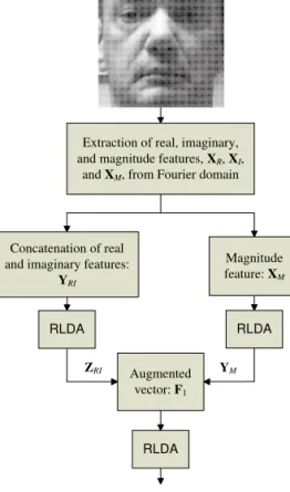
2.1 System architecture of the proposed method. .…..………...………….. 31
2.2 The 2D discrete Fourier transform of a face image: the real part (log plot), the imaginary part, and the magnitude (log plot). The frequency features used in the method are extracted from the right two quadrants, as indicated by the gray
area. …………...………. 32
2.3 The multiple frequency features fusion scheme for the R component image. ..…. 33
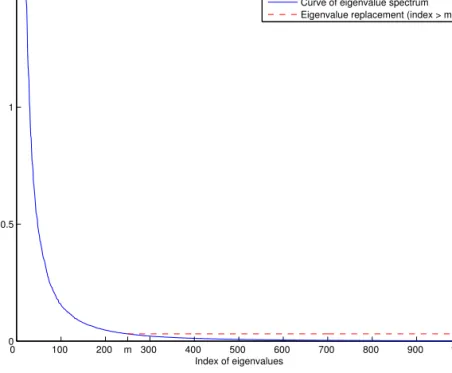
2.4 The eigenvalue spectrum of S′w. While the large eigenvalues are unchanged,
the small eigenvalues with indices larger than m are replaced by a constant,
1
+ =
λ
mρ
, whereλ
m +1 is the (m+1)th eigenvalue in the eigenvalue spectrumof S'w. ..……….. 36
2.5 The face verification rates (ROC III) at 0.1% false accept rate of the R and Y component images using different fusion strategies to fuse the real part, the
imaginary part, and the magnitude. ………...…….. 40
LIST OF FIGURES (Continued)
Figure Page
2.6 Example FRGC images used in experiments that are already cropped to the size
of with two different scales, the scale 1 in the top row and the scale 2 in
the bottom row. In particular, the images from left to right are the R, Y, I, and Q component images, respectively. …………...………...……….
64
64×
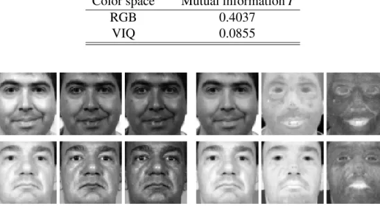
41 3.1 Color component images for two subjects in the FERET (top row) and FGRC
(bottom row) databases, respectively. From left to right, color component
images: R, G, B, V, I, and Q. ...……….………. 47
3.2 Three LBP histograms corresponding to the three LBP operators: , , and , in a subwindow of 2 1 , 8u LBP 2 2 , 8 u LBP LBP8u,32 9×9 pixels. …...………. 48
3.3 Multi-resolution LBP feature fusion scheme. ……… 49
3.4 Discrete-cosine basis functions for N = 4. ………...…... 51
3.5 The diagram of illumination normalization procedures. ……..………..…… 52
3.6 Examples of the illumination normalized gray-scale images. The first column: original gray images; the second column: IDCT reconstructed images in the logarithm domain: the last column: the normalized images after DoG filtering and contrast equalization. ..………...…….. 52
4.1 The color component images R, G, and B (top row), and the new color component images D1, D2, and D3 (bottom row) for one subject. ...………..….. 63
GIR derived from the convolution of one D1 face image with the Gabor kernel with five scales and eight orientations. …….…..………...……… 4.2 64 4.3 The extraction of local and global Gabor features from GIR for face recognition. ………...…. 65
4.4 A reshaped sub-GIR patch image with i∈{1,2,3,4}, and a subset of frequencies in the DCT domain to encode the sub-GIR patch images. .………... 65
The forehead, right cheek and left cheek regions on one D2 image and their
average standard deviations of intensity values of all the D1 and D2 training
images. ………..………...…….. 4.5
66
LIST OF FIGURES (Continued)
Figure Page
4.6 The comparison of the LBP histograms in a window on face images. The top
two rows are the target and query D1 component images of one subject. The
bottom two rows are their associated D2 component images. ………... 67
4.7 Multi-resolution LBP feature fusion scheme. ……...………....………. 68
DCT-based multiple face encoding scheme for the D3 image. ……….….
4.8 69
4.9 The performance of the CID color space vs. the number of principal
components. ………..………. 71
5.1 The patch-based novel image representation. The left image: the partition of an original image. The middle image: a novel representation derived from the color configuration YCrQ based on a patch scheme. The right image: the U-based
representation (gray region) and the D-based representation (dark region). ….… 87
5.2 Architecture of face recognition using the patch-based novel image
representation. ………...…... 89
5.3 Multi-resolution LBP feature fusion scheme. ………….……..……….…… 90
5.4 The image representation from the first column to the sixth column: R, G, and
B; Y, I, and Q; V, Cb, and Cr; UYCrQ, UVCrQ, and UVIQ; DYCrQ, DVCrQ, and DVIQ;
the image derived from YCrQ and RGB using CID model (Yang et al. 2008). … 93
5.5 The ROC curves that are obtained using the proposed method from the
classification outputs of the holistic and local features, as well as their fusion at the decision level via the sum rule. The curves derived from the FRGC baseline
algorithm using the gray-scale images are also included for comparison. ..…….. 96
INTRODUCTION
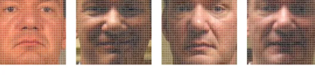
Face recognition, a typical problem in computer vision, pattern recognition, and machine learning, has been attracting more and more research attention recently, due to the complex-ity of the problem itself and the enormous applications in the commercial and government sectors (Bowyer et al. 2006; Zhao et al. 2003; Jain et al. 2004). Although numerous meth-ods in face recognition have been proposed in the last two decades, there are still many open problems that remain to be unsolved. The recent Face Recognition Grand Challenge (FRGC) program reveals that uncontrolled conditions, such as illumination, expression, blurring, and so on, pose grand challenges to face recognition performance (Phillips et al. 2005). Some of the typical image variations on face images are shown in Figure 1.1. Therefore, some new techniques are in great demand to achieve a breakthrough in solving these obstacles. In this chapter, some popular face recognition approaches will be briefly introduced first, and then the outline of the work in this dissertation will be presented.
1.1 Face Recognition Using Appearance-based Methods
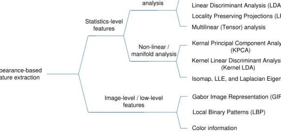
Pattern recognition relies heavily on the particular choice of features utilized by the sifiers. Therefore, feature selection and feature extraction are crucial to many pattern clas-sification problems, e.g., face recognition. One typical block diagram of face recognition system is shown in Figure 1.2. The common objective of feature selection and extraction is to map the original measurements into more effective features, which show significant differences from one class to another, so that the classifiers can be designed more eas-ily with better performance (Fukunaga 1990). One of the dominant and most successful approaches in face recognition is appearance-based feature extraction. Figure 1.3 shows some major methods in this category, which consists of two aspects: statistics-level and
Figure 1.1 Examples of face image variations. Large image variations in illumination, expression, and blurring pose challenges to face recognition.
Face image
Image-level / low-level features
Classifier Statistics-level features
Figure 1.2 Block diagram of face recognition system.
image-level features. Another important category is model-based feature extraction, which utilizes the shape, texture, and 3D depth information for face recognition. More details about these methods can be found in a survey (Lu 2003). In this section, some state-of-the-art face recognition methods belonging to the first category are briefly presented, because the work in this dissertation mainly makes use of features derived from holistic and local face appearance.
1.1.1 Statistics-level Feature Extraction
The face images reside usually in a high-dimensional image space. There is a great de-mand to find the meaningful and compact patterns in such a space for developing robust face recognition methods so as to meet two requirements: enhanced discrimination ability and computational efficiency. Therefore, most appearance-based face recognition
algo-Statistics-level features Appearance-based feature extraction Image-level / low-level features Linear subspace analysis
Principal Component Analysis (PCA) Linear Discriminant Analysis (LDA) Locality Preserving Projections (LPP) Multilinear (Tensor) analysis Kernal Principal Component Analysis
(KPCA)
Kernel Linear Discriminant Analysis (Kernel LDA)
Isomap, LLE, and Laplacian Eigenmap Non-linear /
manifold analysis
Gabor Image Representation (GIR) Local Binary Patterns (LBP) Color information
Figure 1.3 Hierarchical structure of the appearance-based feature extraction in face recog-nition.
rithms usually start with the dimensionality reduction by using some popular linear sub-space methods. In the following sections, several major statistical methods are introduced.
Principal Component Analysis (PCA)
As an optimal linear transformation in the sense of minimum Mean Square Error (MSE), Principal Component Analysis (PCA) (Turk & Pentland 1991; Kirby & Sirovich 1990) has been a leading technique for dimensionality reduction of input data. Given a set ofd-dimensional column image vectors{Xi j}, whereXi j∈Rd is thej-th image of classi.
Let the training set consist ofcpersons andlisample images for personi. Thus, the number of training samples ism=∑ ci=1li. For face recognition, each person is a class with prior probability ofλi. The within-class scatter matrix is defined as:
Sw= c
∑
i=1 λi li li∑
j=1 (Xi j−Xi)(Xi j−Xi)T, (1.1)whereXi= 1li∑ lji=1Xi jis the mean of personi. The between-class scatter matrixSband the total (mixture) scatter matrixSt are defined respectively as:
Sb= c
∑
i=1 λi(Xi−X)(Xi−X)T, (1.2) St= c∑
i=1 λi li li∑
j=1 (Xi j−X)(Xi j−X)T, (1.3) whereX = m1∑ ci=1∑ lij=1Xi jis the grand mean.
PCA seeks a principal subspace of lower dimensionality to maximize the data re-construction capability of the features. As a result, the features in this subspace can repre-sent the original data accurately. The objective function of PCA can be defined as:
W∗=argmax
kWk=1 |W
TS
tW|. (1.4)
Maximizing the above equation can be solved via eigenvalue-eigenvector analysis. That is, the matrixW∗can be constructed by obtaining thekprincipal eigenvectors corresponding
to theklargest eigenvalues ofSt.
Linear Discriminant Analysis (LDA)
The best representation of data may not perform well from the classification point of view, as the total scatter matrix consists of both the within- and between-class variations. To obtain the discrimination of features for differentiating face images of one person from the others, one needs to manipulate the within- and between-class variations separately. To that end, face recognition using Linear Discriminant Analysis (LDA) (Swets & Weng 1996; Belhumeur et al. 1997; Etemad et al. 1997) has been an area of increasing interest. LDA is also known as Fisher Linear Discriminant (FLD). In this dissertation, the terms LDA and FLD are used interchangeably. The objective function of LDA can be defined as:
W∗=argmax
W
|WTSbW|
Equation (1.5) is called the Fisher criterion. To maximize the ratio value of this criterion, LDA seeks an optimal subspaceW∗ that separates the different classes as far as possible
and compresses the same classes as compactly as possible. To derive W∗, LDA solves
the generalized eigenvectors of SbW =λSwW, and chooses the k principal eigenvectors corresponding to theklargest eigenvalues.
Locality Preserving Projections (LPP)
While PCA and LDA aim to preserve the global Euclidean structure, the local man-ifold structure is more important in many real-world applications, especially when nearest-neighbor based classifiers are used for classification (He et al. 2005). Given the high-dimensional data lies on a low high-dimensional manifold embedded in the ambient space, a novel linear learning algorithm, called Locality Preserving Projections (LPP) (He et al. 2005), has been proposed to find an optimal linear transformation to preserve the local ge-ometric structure of the face image space. The objective function of LPP is as follows (He et al. 2005):
min
∑
i j kyi−yjk2Si j, (1.6)
whereyiis the one-dimensional representation ofXiby the linear transformationyi=WTXi. The matrixSis a similarity matrix. A possible way to defineSis given as (He et al. 2005):
Si j= exp(−kXi−Xjk2/t) kXi−Xjk2<ε 0 otherwise, (1.7)
whereε>0 is very small and defines the radius of the local neighborhood. As the neigh-boring pointsXiandXjare mapped far apart, i.e.,kyi−yjk2is large, the objective function incurs a heavy penalty. Therefore, minimizing (1.6) makes an effort to ensure that, ifXi andXjare close, thenyiandyjare close as well (He et al. 2005).
DefiningDas a diagonal matrix whose entries are column (or row sinceSis sym-metric) sums of S, i.e., Dii=∑ jSji (He et al. 2005), one can derive Laplacian matrix as
L=D−S. Following some simple algebraic steps, the objective function (1.6) is rewritten
as:
W∗=argmin
W W
TXLXTW s.t.WTXDXW =1. (1.8)
The optimal transformation vectorW can be derived by the minimum eigenvalue solution to the generalized eigenvector problem: XLXTW =λXDXTW. By using LPP, a new face
recognition method called Laplacianfaces has been proposed to map the face images into a face subspace for analysis and has demonstrated more discriminative power than Eigen-faces and FisherEigen-faces for face recognition (He et al. 2005).
Tension-based Image Representation
Currently, most subspace learning methods handle image data in the form of 1-D vectors, by concatenating the columns or rows of an image into a single vector. This process most likely results in the curse of dimensionalitydilemma and the small sample size problem, because the dimensionality of features usually is much larger than the sample size. However, image essentially is matrix, i.e., second-order tensors, which has motivated researchers to propose some novel subspace methods, such as 2-D PCA (Yang et al. 2004) and 2-D LDA (Ye et al. 2004), to extract features directly on images. In recent years, advances have focused on encoding face images as second- or higher-order tensors and extending the traditional PCA, LDA, and LPP into their tensorized versions (Yan et al. 2007a; Yan et al. 2007b; Tao et al. 2007; Xu et al. 2008; Fu & Huang 2008a). These emerging methods have showed the superiority over some traditional subspace learning methods in both recognition accuracy and computational efficiency.
Kernel PCA
Linear analysis methods have met with difficulties in extracting the effective fea-tures for face recognition, when the face images suffer from the large variations due to il-lumination conditions, viewing directions or poses, facial expression, aging, and disguises such as facial hair, glasses, or cosmetics. Encountering these challenges, face recognition schemes are required to possess enhanced discrimination abilities. Since the late 1990s, enormous efforts have been put into developing nonlinear analysis methods (e.g., kernel-based methods). By taking advance of a nonlinear kernel mapping, one is able to improve the discriminating power of the feature representation remarkably.
To obtain higher order correlations beyond variances and covariances between input variables, linear PCA was extended to a nonlinear form, Kernel PCA (KPCA) (Schölkopf et al. 1998). The basic idea of KPCA is mapping the original input space to a high-dimensional feature space, where standard PCA is actually conducted. By applying kernel functions that implement a canonical dot product in the low-dimensional input space in-stead of the high-dimensional feature space, KPCA implicitly achieves the nonlinear map-ping between the input space and the feature space, such that the expensive computation in directly nonlinear mapping is avoided subtly.
Given a set of samples x1,x2, . . . ,xm∈Rd in the input space, the kernel induces a nonlinear mapping between the input space and the feature space denoted byφ : Rd→H.
Then the kernel mapped data is first centered and then is used to form a data matrix in the feature space: D= [φ(x1),φ(x2), . . .,φ(xm)]∈H. LetK∈Rm×mbe a kernel matrix defined
by the dot product in the feature space. The elementKi jinKis given as:
Ki j=k(xi,xj) = (φ(xi)·φ(xj)), (1.9)
wherek(·)is a kernel function and is usually defined as three types: polynomial kernels,
Gaussian kernels, and sigmoid kernels (Schölkopf & Smola 2002). Rather than directly eigen-decomposing the covariance matrix,C=m1 ∑ mi=1φ(xi)φ(xi)t, whose dimensionality is
very high or even infinite in the feature space, Schölkopf et al. (1998) derived the equivalent eigenvalue problem:
mλα =Kα, (1.10)
whereα = [α1,α2, . . .,αm]t is a column vector. Then an eigenvectorV of KPCA is com-puted as follows: V =Dα= m
∑
i=1 αiφ(xi). (1.11)Given a training/test sample x, the corresponding feature in the feature space is φ(x). Thek-th KPCA feature ofxis computed as the projection ofφ(x)onto the eigenvector Vk: β(x)k=Vkφ(x) = m
∑
i=1 αk iK(xi,x). (1.12) Kernel LDASimilar to linear PCA, KPCA still captures only the overall variance of input pat-terns, which is not significant for discrimination purpose. To account for the nonlinear interactions among patterns, linear LDA needs to be extended to a nonlinear form, ker-nel LDA, to obtain the enhanced discrimination power. The idea of kerker-nel LDA was first proposed by Mika et al. (1999), whose method deals with two-class pattern classification problems. Subsequently, Baudat and Anouar (2000) proposed another type of kernel LDA, called Generalized Discriminant Analysis (GDA), to address multiclass pattern classifica-tion problems. Since then, research has witnessed the development of a bunch of kernel LDA algorithms (Roth & Steinhage 2000; Cooke 2002; Yang et al. 2002; Lu et al. 2003; Yang et al. 2005). Thus, there are several kinds of kernel LDA formulations. One among them is called KPCA + LDA (Yang et al. 2005), whose straightforward insight into the na-ture of kernel LDA makes it easier to understand and implement kernel LDA, particularly
for new investigators and programmers (Yang et al. 2005).
As revealed in Yang’s paper, the essence of kernel LDA consists of two steps. That is, KPCA is first used to reduce (or increase) the dimensionality of the input space to n, which is the rank of the covariance matrix C in the feature space, i.e., the rank of the centralized Gram matrixK defined in Equation (1.9). Generally,n=m−1, wheremis the
number of training samples. Next, LDA is implemented for further feature extraction in the KPCA-transformed space Rn (Yang et al. 2005). Letyi j be the KPCA feature of the j-th training sample in classi, calculated by Equation (1.12). The within- and between-class scatter matrices inRnare defined as:
Sw= c
∑
i=1 λi li li∑
j=1 (yi j−yi)(yi j−yi)T, (1.13) Sb= c∑
i=1 λi(yi−y)(yi−y)T, (1.14)whereli is the number of training samples in classi with prior probability ofλi, yi is the mean of the training samples in classi,yis the grand mean. The ordinary LDA procedures then derive an optimal transformation matrix U. Finally, given a training/test image, its kernel LDA features are defined as:
Z=UtVtφ(x) =UtΩtΘ, (1.15)
where Ωand Θhave similar definitions as α and K(xi,x) in KPCA. Please refer to the paper (Yang et al. 2005) for more details.
Manifold Learning
For conducting nonlinear dimensionality reduction on the high-dimensional data that can be considered as a set of geometrically correlated points lying on or nearly on a smooth low-dimensional manifold, some popular manifold learning algorithms include
Lo-cally Linear Embedding (LLE) (Roweis & Saul 2000), Isomap (Tenenbaum et al. 2000), Laplacian Eigenmaps (LE) (Belkin & Niyogi 2003) have recently been developed. LLE maps the input data to a lower dimensional space in a manner that preserves the relation-ship between the neighboring points; Isomap finds the low-dimensional representations for a data set by approximately preserving the geodesic distances of the data pairs; LE pre-serves the similarities of the neighboring points, and its linearized form is LPP. Although these algorithms are derived on the basis of different motivations, they all can be unified within the Graph Embedding (GE) framework and its linear/kernel/tensor extensions (Yan et al. 2007). These nonlinear methods do yield impressive results on some benchmark ar-tificial data sets. However, the generated maps are defined only on the training data points, and how to evaluate the maps on novel test data points remains unclear (He et al. 2005). Therefore, these nonlinear manifold learning algorithms might not be suitable for some computer vision tasks, such as face recognition (He et al. 2005).
Recent studies also reveal that locality features and intrinsic geometric structures in the input space may take on additional discriminating power for classification, assum-ing that Locally Embedded Analysis (LEA) (Fu & Huang, 2005), and Locally Preservassum-ing Projections (LPP) (He et al., 2005). Both nonlinear kernel mapping and locally preserved graph embedding help improve the discriminating power of feature representation. How-ever, they generally have the drawback of high-computational cost in classification and overfitting (Fu et al., 2008; Kim et al., 2005).
1.1.2 Image-level Feature Extraction
Image variations cause the changes of data distribution in high-dimensional image space. If raw images are used directly for face recognition, such changes pose burden to the process of statistical feature extraction via either linear or nonlinear way. To facilitate the statistical feature extraction for classification, some image feature extraction techniques have been developed to process raw images for extracting image features, which are usually invariant
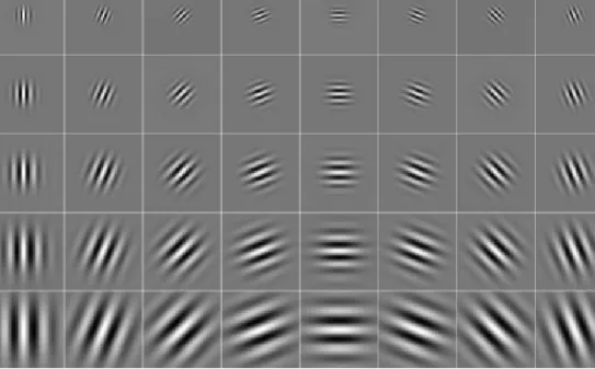
Figure 1.4 Gabor wavelets: the real part of the Gabor kernels at five scales and eight
orientations.
to image variations. Some popular methods in image feature extraction include Gabor Image Representation (GIR) (Daugman 1985; Donato et al. 1999; Liu & Wechsler 2002), and Local Binary Patterns (LBP) (Ojala et al. 1996; Ojala et al. 2002).
Gabor Image Representation (GIR)
GIR of an image captures salient visual properties such as spatial location, orien-tation selectivity, and spatial frequency characteristics (Daugman 1985), displaying robust characteristics in dealing with image variabilities. Specifically, GIR is the convolution of the image with a family of Gabor kernels that may be formulated as follows (Daugman 1985): ψµ,ν(z) = k kµ,νk2 σ2 e− kkµ,νk2kzk2 2σ2 eikµ,νz−e−σ22 (1.16) whereµ andν define the orientation and scale of the Gabor kernels,z= (x,y),k · kdenotes
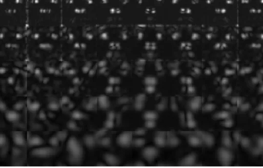
Figure 1.5 Gabor image representation (GIR): the magnitude representation.
kµ,ν =kνeiφµ (1.17)
wherekν =kmax/fν andφµ=πµ/8. kmax is the maximum frequency, and f is the spacing factor between kernels in the frequency domain. Let I(x,y) represent a face image, the
convolution ofI(x,y)and a Gabor kernelψµ,ν may be formulated as follows:
Oµ,ν(z) =I(z)∗ψµ,ν(z) (1.18)
wherez= (x,y),∗denotes the convolution operator, and Oµ,ν(z)is the convolution result corresponding to the Gabor kernel at orientation µ and scale ν. Commonly used Gabor kernels contain five different scales, ν ∈ {0, ...,4}, and eight orientations, µ ∈ {0, ...,7}. The set S ={Oµ,ν(z):µ ∈ {0, ...,7},ν ∈ {0, ...,4}}, thus, forms GIR of the image I.
Figure 1.4 shows the the real part of Gabor kernels at different scales and orientations, and Figure 1.5 shows the magnitude of GIR derived from the convolution of a face image with these Gabor kernels. Usually, the concatenated magnitude images are considered as Gabor features for face recognition (Liu et al. 2002).
Figure 1.6 An example of the basic LBP operation (Ahonen et al. 2006).
Figure 1.7 An example of LBP circular neighborhoods: (8,1), (16,2), and (8,2). When
the sampling point is not at the center of a pixel, the pixel value is bilinearly interpolated.
Local Binary Patterns (LBP)
LBP, which was originally introduced for texture analysis (Ojala et al. 1996), has been successfully extended to describe face images and demonstrated effective for face recognition, due to the finding that face images can be viewed as a composition of micro-patterns that are well described by the LBP operators. In a 3×3 neighborhood of an
image, the basic LBP operator assigns a binary label 0 or 1 to each surrounding pixel by thresholding at the gray value of the central pixel and replacing its value with a decimal number converted from the 8-bit binary number. Formally, the LBP operator is defined as follows: LBP= 7
∑
p=0 2ps(ip−ic) (1.19)wheres(ip−ic)equals 1, ifip−ic≥0; and 0, otherwise. Figure 1.6 illustrates an example of the basic LBP operator.
Two extensions of the basic LBP were further developed by Ojala et al. (2002). The first extension allows LBP to deal with any size of neighborhoods by using circular neigh-borhoods and bilinearly interpolating the pixel values. The notation (P,R) thus represents
The second extension defines the so calleduniform patterns. When the binary string is traversed circularly, LBP can be called uniform if there are at most two bitwise transitions from 0 to 1 or vice versa. For example, the patterns 00000000 (0 transitions), 00011100 (2 transitions) and 11000011 (2 transitions) are uniform whereas the patterns 11010011 (4 transitions) and 00101001 (6 transitions) are not. In the computation of LBP histograms, every uniform pattern has its own bin and all nonuniform patterns are assigned to a separate bin. Ahonen et al. (2006) have found that 90.6% of the patterns in the (8,1) neighborhood and 85.2% of the patterns in the (8,2) neighborhood are uniform when processing FERET facial images. After extensions, LBP can be expressed as: LBPu2
P,R.
1.1.3 Color Information for Face Recognition
Most existing face recognition methods work with the gray-scale images, which have been revealed to be suffering from severe image variations by the recent Face Recognition Grand Challenge (FRGC) program (Phillips et al. 2005). Color information has been widely applied in face detection, but not in face recognition. Recent studies show that different color spaces transformed from the RGB color space display different discriminating power for pattern recognition (Hsu et al. 2002; Geusebroek et al. 2001; Torres et al. 1999; Ross & Govindarajan 2005; Shih et al. 2005). As different color component images in a color space exhibit the various representations of faces, they could provide the complementary information to each other. Such a characteristic implies that when some facial features produce the incorrect classification output due to image variations on the luminance-related images, such as Y, R, and V of HSV, they could work well on the chromatic images, such as I, Q, Cr, and so on. As a result, the sets of face images misclassified by the different color component images would not necessarily overlap. Therefore, data fusion at the image level or the decision level can be used to combine several color component images to improve the performance of face recognition, when compared to the methods using gray-scale images alone.
There are a few approaches in the literature to address the feature extraction in color space. Xie and Kumar (2005) proposed the quaternion correlation filter technique for color face recognition that processes all of the color channels jointly, where the quaternion repre-sentation encodes the three color components (such as in the RGB and NTSC color spaces) in the imaginary parts of the quaternion number. Jones and Abbott (2006) further proposed to use the quaternion representation to extend the Gabor filters from the complex domain to the hypercomplex domain for color face recognition. To overcome the large illumination variations on color in face images, Kim and Choi (2007) proposed the construction of a tensor of color image ensemble. They formed a 4-way tensor whose coordinates are asso-ciated with rows and columns of face images, color, and samples, and then employed the higher-order SVD of the tensor to extract such features. The other approaches of extracting features in color face images include the application of Non-negative Matrix Factorization (NMF) (Rajapakse et al. 2004) and LBP (Chan et al. 2007).
This section first details ten commonly used color spaces in computer vision and pattern recognition, then introduces an emerging technique of color space normalization in face recognition. The ten color spaces include: the RGB color space, thergbcolor space, the I1I2I3 (decorrelated RGB) color space, the human perceptual color spaces HSV and
HSI, the video transmission efficiency color spaces YIQ, YUV and YCbCr, the CIE-XYZ color space, and the CIE perceptually uniform color space CIE-L∗a∗b∗.
The rgb color space
The RGB colors are sensitive to surface orientation, illumination direction, and illumination intensity. To alleviate such sensitivities, one can derive the normalized colors by projecting the R, G, B values onto the R = G = B = max{R,G,B} plane. The projection spans a normalizedrgbchromaticity triangle. The transformation is defined as:
r=R/(R+G+B) g=G/(R+G+B) b=B/(R+G+B).
(1.20)
The I1I2I3color space
An effective color space to stabilize RGB images is I1I2I3, proposed by Ohta et al.
(1980), which uses Karhunen-Loève transformation (KLT) to decorrelate the RGB compo-nents. The conversion from RGB to I1I2I3based on Ohta’s experimental model is given by
the simple linear transformation:
I1 I2 I3 = 1/3 1/3 1/3 1/2 0 −1/2 −1/2 1 −1/2 R G B . (1.21)
Human perceptual color spaces
The HSI and HSV color spaces are motivated by the human vision system in a sense that one can describe color by means of hue, saturation, and brightness. Hue and saturation define chrominance, while intensity or value specifies luminance. The HSI color space is defined as follows: I= (R+G+B)/3 S=1−(1/I)min(R,G,B) H= θ ifB≤G 360−θ otherwise, (1.22) where
θ =cos−1 ( 1 2[(R−G) + (R−B)] [(R−G)2+ (R−G)(G−B)]21 ) . (1.23)
The HSV color space is defined as:
Let MAX = max(R,G,B) MIN = min(R,G,B) δ = MAX−MIN H= 60(G−δB) if MAX=R 60(B−δR+2) if MAX=G 60(R−δG+4) if MAX=B
not defined if MAX=0
S= δ MAX if MAX6=0 0 if MAX=0 V =MAX. (1.24)
In order to confine H within the range of [0,360],
H=H+360 if H<0. (1.25)
Note that the R, G, B values in both Equations (1.22) and (1.24) are scaled to[0,1].
Video transmission efficiency color spaces
The YUV and YIQ color spaces are widely used in video for transmission effi-ciency. The YUV color space is applied by Phase Alternation by Line (PAL) and the Sys-tem Electronique Couleur Avec Memoire (SECAM), and the YIQ color space is adopted by the National Television System Committee (NTSC) video standard in reference to RGB NTSC. The YUV color space is defined as:
Y U V = 0.2990 0.5870 0.1140 −0.1471 −0.2888 0.4359 0.6148 −0.5148 −0.1000 R G B . (1.26)
The I and Q components are derived from their counterparts, U and V, by a clock-wise rotation (33o), and then the YIQ color space is defined as follows:
Y I Q = 0.2990 0.5870 0.1140 0.5957 −0.2745 −0.3213 0.2115 −0.5226 0.3111 R G B . (1.27)
The YCbCr color space is a scaled and offset version of the YUV color space. To derive YCbCr, the RGB components are distributed into luminance (Y), chrominance blue (Cb), and chrominance red (Cr). The Y component has 220 levels ranging from 16 to 235, while the Cb, Cr components have 225 levels ranging from 16 to 240:
Y Cb Cr = 16 128 128 + 65.4810 128.5530 24.9660 −37.7745 −74.1592 111.9337 111.9581 −93.7509 −18.2072 R G B . (1.28)
where the R, G, B values are scaled to[0,1].
CIE uniform color spaces
In the CIE (Commission Internationale de 1’Éclairage) systems, the starting point for all color specification is CIE XYZ. XYZ is known as tristimulus values, which lead to the other CIE perceptually uniform color spaces, such as the L∗a∗b∗color space. A linear
transformation from RGB space to XYZ space is defined as: X Y Z = 0.607 0.174 0.201 0.229 0.587 0.114 0.000 0.066 1.116 R G B . (1.29)
The L∗a∗b∗ color space is one of the most popular color spaces and is modeled
based on the human vision system. The L∗component represents brightness from 0 (black)
to 100 (white). The a∗ component corresponds to the measurement of redness (positive
values) or greenness (negative values), and the b∗component corresponds to the
measure-ment of yellowness (positive values) and blueness (negative values). Based on the XYZ tristimulus, the L∗a∗b∗color space is defined as:
L∗=116f(Y Yo)−16 a∗=500hf(X Xo)−f( Y Yo) i b∗=200hf(Y Yo)−f( Z Zo) i (1.30) where f(x) = x1/3 ifx>0.008856 7.787x+11616 otherwise. (1.31)
In addition to the above existing color spaces, a few researchers have devoted to generating some new color spaces for face recognition (Jones III & Abbott 2004; Liu 2008; Yang et al. 2008; Liu & Yang 2009). The main idea of these methods can be described as: first, the color-space total, between-class, and within-class scatter matrices are constructed using pixel values containing different color components, then some linear learning algo-rithms, such as PCA, LDA, and Independent Component Analysis (ICA), are applied to these scatter matrices to derive the transformation vectors, which generate one or several new color components from original color components. The motivation behind generating new color spaces is to make the new color components more uncorrelated, more
discrimina-tive, and more independent than original color components for improving the performance of face recognition.
Color Space Normalization for Face Recognition
The most important issue of color-based face recognition is to choose the appropri-ate color spaces, which are able to provide more discriminative power than the others. As a straightforward way, the exhaustive enumeration strategy has been applied in the refer-ence (Shih et al. 2005) to seek the best color spaces. Their research reveals that different color spaces transformed from the RGB color display different discriminating abilities for face recognition. Specifically, the YIQ color space provides better face recognition perfor-mance in comparison with other color spaces. One nature question arises “what kind of color spaces is suitable for color face recognition?", namely, what characteristics are re-lated to the discriminative color spaces for face recognition? To answer this question, Yang et al. (2010b) have proposed the concept of Double-Zeros-Sum (DZS) in color spaces.
By discovering what characteristics make the I1I2I3, YUV, and YIQ color spaces
more powerful than the RGB and XYZ color spaces for face classification, Yang et al. (2010a) found an interesting observation in color transformation matrices: the sums of the elements in the second and third rows of the transformation matrix are both zero or approx-imate zero. This characteristic is so called Double-Zeros-Sum (DZS) (Yang et al. 2010b). However, the RGB and XYZ color spaces do not hold such a property. For example, the transformation matrix of the RGB color space is given as follows:
R G B = 1 0 0 0 1 0 0 0 1 R G B . (1.32)
in second and third rows are not zero. A similar situation also appears in other weak discriminating color spaces, such as XYZ.
Inspired by this finding, Yang et al. (2010a) further proposed the concept of color space normalization (CSN) and developed two CSN techniques. These CSN techniques can work well in all color spaces that are derived by a linear transformation of the RGB color space, so that the normalized color spaces possess the same property as the strong discrim-inating color spaces. The two normalization techniques, according to whether the com-putation procedures happen within a color component or across three color components, are named aswithin-color-componentnormalization (CSN-I) andacross-color-component
normalization (CSN-II), respectively. Next, the CSN-I technique will be briefly presented, and readers can refer to the paper (Yang et al. 2010a) for the details of the CSN-II.
Let C1, C2, and C3 be the three color components derived by the following linear
transformation of the RGB color space:
C1 C2 C3 =A R G B = A1 A2 A3 R G B = a11 a12 a13 a21 a22 a23 a31 a32 a33 R G B . (1.33)
The mean values of the second and the third rows inAare m2= (a21+a22+a23)/3 and
m3= (a31+a32+a33)/3, respectively. Subtractingm2 andm3 from the second and third
rows results in a normalized transformation matrix ˜A, which generates a normalized color space ˜C1˜C2˜C3(Yang et al. 2010a):
˜ C1 ˜ C2 ˜ C3 = A˜ R G B = A1 ˜ A2 ˜ A3 R G B = a11 a12 a13 a21−m2 a22−m2 a23−m2 a31−m3 a32−m3 a33−m3 R G B . (1.34)
For example, the normalized RGB and XYZ color spaces via the CSN-I are defined as: ˜ R ˜ G ˜ B = 1 0 0 −1/3 2/3 −1/3 −1/3 −1/3 2/3 R G B , ˜ X ˜ Y ˜ Z = 0.607 0.174 0.201 −0.0343 0.2537 −0.2193 −0.3940 −0.3280 0.7220 R G B . (1.35)
Some Preliminary Evaluations of Different Color Spaces for Face Recognition
To evaluate the feasibility of color information in face recognition, a set of experiments has been executed on the FRGC version 2 Experiment 4, the most challenging FRGC exper-iment, which contains 12,776 face images of 222 subjects in the training set, 16,028 face images of 466 subjects in target set, and 8,014 face images of 466 subjects in the query set. Image normalization is first used to align the centers of the eyes to specified positions and fixed interocular distance. To be specific, the centers of the eyes are provided by the FRGC
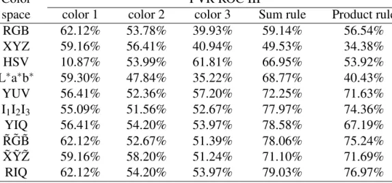
Table 1.1 Face Verification Rate (FVR) ROC III of the FRGC Database Using Several Different Color Spaces
Color FVR ROC III
space color 1 color 2 color 3 Sum rule Product rule
RGB 62.12% 53.78% 39.93% 59.14% 56.54% XYZ 59.16% 56.41% 40.94% 49.53% 34.38% HSV 10.87% 53.99% 61.81% 66.95% 53.92% L∗a∗b∗ 59.30% 47.84% 35.22% 68.77% 40.43% YUV 56.41% 52.36% 57.20% 72.25% 71.63% I1I2I3 55.09% 51.56% 52.67% 77.97% 74.36% YIQ 56.41% 54.20% 53.97% 78.58% 67.19% ˜R ˜G ˜B 62.12% 52.67% 51.39% 78.06% 75.24% ˜X ˜Y˜Z 59.16% 58.20% 51.24% 71.10% 71.69% RIQ 62.12% 54.20% 53.97% 79.03% 76.97%
database and the predefined positions in the 64×64 images are (17, 18) and (47, 18). A
subimage procedure then crops the face image to the size of 64×64 to extract the facial
region. Some example images are shown in Figure 1.1. Finally, an LDA-based algorithm and the cosine similarity measure are implemented to recognize faces.
The classification results of individual color components are first derived, and then the sum rule and the product rule are applied, respectively, to fuse these classification outputs for deriving the performance of color spaces for face recognition. Experimental results using the different color spaces are derived from the Receiver Operating Character-istic (ROC) curves. Table 1.1 summarizes the Face Verification Rate (FVR) from the ROC III curves. As can be seen, when the FVR (56.41%) of the luminance Y is considered as benchmark, most of color spaces improve the face recognition performance significantly. In particular, some strong discriminating color spaces, such as YIQ, I1I2I3, YUV, can achieve
good performance in face recognition, while some weak discriminating color spaces, such as RGB and XYZ, achieve low performance. On the other hand, experimental results show that the color normalization technique indeed causes the weak color spaces RGB and XYZ to enhance the discrimination for face recognition. In addition, two nonlinear color spaces
HSV and L∗a∗b∗do not demonstrate any advantage over some strong discriminating color
spaces. It should be noted that the hybrid color spaces, such as RIQ, demonstrate the ad-vantage in improving recognition performance over other color spaces.
1.2 Topics Overview
Most of the existing color-based face recognition methods pay attention to the selection and generation of color spaces, largely ignoring the research on the low-level feature extraction in different color spaces. For example, the paper (Shih et al. 2005) assesses comparatively face recognition performance in different color spaces using a standard PCA algorithm. The research reveals that some color configurations, such as YV in the YUV color space and YI in the YIQ color spaces, can help improve face recognition performance. How-ever, nothing about the low-level feature extraction has been investigated in this paper. To fill in such a gap, this dissertation focuses on face recognition by addressing facial feature extractions in different color component images. Specifically, some image feature extrac-tion methods have been investigated and developed to extract the effective features from color images for face recognition. The feasibility and effectiveness of the proposed meth-ods have been evaluated by two large-scale face databases, namely, the Face Recognition Grand Challenge (FRGC) version 2 database and the FERET database. The FRGC ver-sion 2.0 Experiment 4, the most challenging FRGC experiment, contains 12,776 training images, 16,028 controlled target images, and 8,014 uncontrolled query images. To assess the generalization of the proposed methods, the experiments using the FERET database are also conducted. The two most challenging probe sets, Dup I and Dup II, which are used for analyzing the effect of aging on the recognition performance, are evaluated in the ex-periments. The Biometric Experimentation Environment (BEE) system of FRGC and the rank-1 accuracy rate of FERET reveal that the proposed methods improve performance of face recognition significantly, which not only take advantages over the traditional methods using gray-scale images but also outperform some state-of-the-art face recognition
meth-ods.
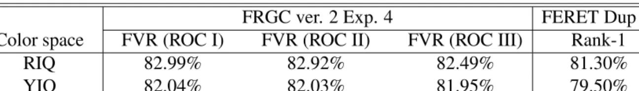
Chapter 2 presents a novel multiple feature fusion method for face recognition by fusing the frequency, spatial, and color features for improving the face recognition grand challenge performance. In particular, the hybrid color space RIQ is constructed, accord-ing to the discriminataccord-ing properties among the individual component images. For each component image, the frequency features are extracted from the magnitude, the real and imaginary parts in the frequency domain of an image. Then, a variant of Regularized Lin-ear Discriminant Analysis (RLDA) extracts discriminating features from the frequency data for similarity computation using a cosine similarity measure. Finally, the three similarity matrices generated using the three components in the RIQ color space are fused by means of the sum rule — the decision level fusion — to derive the final similarity matrix for face recognition. The effectiveness of the proposed method is demonstrated using two large-scale face databases, namely, the FRGC version 2 and the FERET databases. In particular, experiments on FRGC and BEE show that for the most challenging FRGC version 2 Exper-iment 4, the proposed method achieves the face verification rate (ROC III) of 82.49% at the false accept rate of 0.1%. For the FERET Dup I probe set, the proposed method achieves the rank-1 accuracy of 81.30%.
Chapter 3 describes a novel face recognition method, embodying the “Color + LBP + LDA” strategy. First, another hybrid color space VIQ is constructed by replacing the luminance Y in YIQ by the V component in HSV. As there is more mutual independence information in VIQ than in the RGB, the hybrid VIQ color space is more feasible as a com-plementary representation of face images for classification than some color spaces, such as RGB. On each component image of VIQ, a multipscale LBP fusion is proposed to en-compass the different LBP histogram features. By utilizing such a fusion scheme, both the microstructures and macrostructures of face images are fused to extract the discriminating features, which can contain much more discrimination information than the one a single LBP operator can provide. Regarding the extraction of discriminating features, a variant
of RLDA is used to extract the complete discriminating information, which resides in both the principal and null spaces of the within-class scatter matrix. Experiments on the FRGC version 2 and FERET databases show that the proposed method using the “Color + LBP + LDA” strategy can significantly improve face recognition performance under difficult conditions.
Chapter 4 is concerned with the application of different feature extraction meth-ods to different color component images. Now that the different color component images display the various discriminating properties and face representations, it is more feasible to apply a variety of feature extraction methods than the single-feature extraction methods to some color component images for face recognition. This chapter first introduces the derivation of a new color space, the Color Image Discriminant (CID) color space (Yang et al. 2008). Then an emphasis is laid on using Gabor Image Representation (GIR), Local Binary Patterns (LBP), and the frequency features in the different color component images of the CID color space, respectively, for improving the performance of face recognition. In particular, experiments on the FRGC data set show that the proposed method can achieve the FVR of 91.6% at 0.1% FAR.
Chapter 5 discusses the generation of some new image representations for face recognition. Most existing face recognition methods use the gray-scale image, which is the simple linear combination of the primary colors R, G, and B. However, the disadvantage of such an usage is that R, G, and B have strong correlation to each other. Since the decorrelation property is essential for pattern recognition, the image representations derived from three primary color components are not ideally suited for face recognition. This chapter first derives some new image representations from the other color spaces through a learning algorithm, and then proposes a novel method for addressing the problem of face recognition under the difficult illumination conditions. Experiments on two large-scale face databases, FRGC and FERET, show the effectiveness of the proposed method.