(will be inserted by the editor)
Partitioning predictors in multivariate regression models
Francesca Martella · Donatella Vicari · Maurizio Vichi
Received: date / Accepted: date
Abstract A Multivariate Regression Model Based on the Optimal Partition of Predictors (MRBOP) useful in applications in the presence of strongly correlated pre-dictors is presented. Such classes of prepre-dictors are syn-thesized by latent factors, which are obtained through an appropriate linear combination of the original vari-ables and are forced to be weakly correlated. Specifi-cally, the proposed model assumes that the latent fac-tors are determined by subsets of predicfac-tors charac-terizing only one latent factor. MRBOP is formalized in a least squares framework optimizing a penalized quadratic objective function through an alternating least-squares (ALS) algorithm. The performance of the method-ology is evaluated on simulated and real data sets. Keywords Penalized regression model· Partition of variables· Least squares estimation·Class-correlated variables·Latent factors
1 Introduction
Applications where several dependent variables (respon-ses) have to be predicted using a large number of vari-ables have been considered in various disciplines such as bioinformatics, brain imaging, data mining, genomics Francesca Martella
Dipartimento di Scienze Statistiche, Sapienza Universit`a di Roma, Piazzale Aldo Moro, 5 - 00185 Rome (Italy)
Tel.: +39-06-49910464
E-mail: [email protected] Donatella Vicari
Dipartimento di Scienze Statistiche, Sapienza Universit`a di Roma, Piazzale Aldo Moro, 5 - 00185 Rome (Italy)
Maurizio Vichi
Dipartimento di Scienze Statistiche, Sapienza Universit`a di Roma, Piazzale Aldo Moro, 5 - 00185 Rome (Italy)
and economics (Frank and Friedman, 1993; Waldro et al., 2011). The standard model that accommodates this issue is the ordinary multivariate regression model, see chapter 15 in Krzanowski (2000). Fitting the multivari-ate regression model to observed data requires estima-tion of the unknown regression coefficients and the dis-persion matrix of the error terms. This can be done by maximum likelihood if normality is assumed for the error matrix or by least-squares if no distributional as-sumptions are made. For standard application of the inferential theory, it is necessary for the sample size to be greater than the number of predictors plus the number of responses and for the predictor matrix to be of full rank. However, when the number of predictors is large, two important statistical problems, which are related to each other, may commonly arise:
1. difficulty in interpretation of the (many) regression coefficients;
2. presence of strongly correlated predictors.
In the latter case, the regression approach may still be able to determine the ordinary least squares (OLS) estimators, but it may not be able to distinguish the ef-fect of each predictor on the responses (multicollinear-ity). In the literature many proposals and strategies for dealing with such problems have been proposed, which can be classified into three categories: standard variable selection methods, see as an example Hocking (1976), penalized (or shrinkage) techniques, also known as bias estimation, see Tibshirani (1996); Hoerl and Kennard (1970); Frank and Friedman (1993); Zou and Hastie (2005); Tutz and Ulbricht (2009); Witten and Tibshi-rani (2009); Yuan and Lin (2006), and dimensionality reduction methods (DRMs).
In particular, we focus on DRM regression where a small set of linear combinations of the original
vari-ables are built and then used as input to the regres-sion model. DRMs differ in how the linear combina-tions are built. For example, principal component re-gression (PCR) (Jolliffe, 1982) performs a PCA on the explanatory variables and uses the principal compo-nents as latent predictors in the regression model. It has been demonstrated that this strategy does not guar-antee the principal components, which optimally “ex-plain” the predictors, will be relevant for the predic-tion of the responses. Canonical correlapredic-tion regression (CCR) (Hotelling, 1935) is similar to PCR, but whereas PCR finds the directions of maximal variance of each predictor-space, CCR identifies directions of maximal correlation of both predictor and response spaces. Par-tial least squares regression (PLSR) (Wold, 1966) repre-sents a form of CCR where the criterion of maximal cor-relation is balanced by requiring the model to explain as much variance as possible in both predictor and re-sponse spaces. Stone and Brooks (1990) proposed con-tinuum regression as a unified regression technique em-bracing OLS, PLSR and PCR. On the other hand, Re-duced Rank Regression (RRR) (Anderson, 1951; Izen-man, 1975) minimizes the sum of the squared residuals subject to a reduced rank condition. It can be seen as a regression model with a coefficient matrix of reduced rank. Moreover, it can be shown that the RRR latent predictors are the same as the ones from the Redun-dance Analysis (RA), see Van Den Wollenberg (1977). Yuan et al. (2007) proposed a general formulation for dimensionality reduction and coefficient estimation in multivariate linear regression, which includes many ex-isting DRMs as specific cases. Bougeard et al. (2007) proposed a new formulation to the multiblock setting of latent root regression applied to epidemiological data and Bougeard et al. (2008) investigated a continuum approach between MR and PLS. However, dimension-ality reduction methods, such as PCA and Factor Anal-ysis, may generally suffer from a lack of interpretability of the resulting linear combinations. Rotation methods are often used to overcome such a problem. In the re-gression context, we propose here to simplify the inter-pretation by partitioning the predictors into classes of correlated variables synthesized by weakly correlated factors that best predict the responses in the least-squares sense. This turns out to be a relevant gain in the interpretation of the regression analysis, which can be nicely displayed by a path diagram identifying the underlying relations between predictors, latent factors and responses. The model should be used when the re-searcher does not have a priori hypotheses about the association patterns present between the manifest vari-ables.
In this paper a multivariate regression model based on the optimal partition of predictors (MRBOP) is pro-posed which optimally predict the responses in the least-squares sense. In fact, the assumption underlying the model is the existence of weakly correlated groups of predictors but the number and the composition of such possible blocks need to be determined. In the frame-work of DRMs, the new methodology determines latent factors as linear combinations of such subsets of pre-dictors by performing simultaneously the clustering of the predictors and the estimation of the regression co-efficients of the derived latent factors. Specifically, the model proposed aims at defining classes of correlated predictors, which lead to the construction of weakly cor-related latent factors. This could be particularly useful in high dimensional regression studies where strongly correlated variables might represent an unknown under-lying latent dimension. In these cases, methods that are commonly employed as cures for collinearity - in par-ticular, variable selection - can be inadequate because important grouping (i.e. latent dimension) information may be lost. Moreover, in the case of perfect linear re-lationship among predictors, we can here algebraically derive the regression coefficient estimators contrarily to the OLS framework. Finally, an important advantage of MRBOP is the interpretability of each latent factor representing only one subset of well-characterized pre-dictors. In fact, predictors are not allowed to influence more than one factor as frequently happens in dimen-sionality reduction methods.
The model is formalized in a least squares estima-tion framework optimizing a penalized quadratic objec-tive function. The paper is organized as follows. Section 2 describes the general DRMs and discusses the possi-ble specifications, while Section 3 introduces the model and an alternating least-squares algorithm to estimate the model parameters. An illustrative example is pre-sented in Section 3.2.1. In Sections 4 and 5, the results obtained on simulated and real data sets are discussed. The last Section is devoted to concluding remarks.
2 Dimensionality reduction methods in multivariate regression
LetX= [xij] be a (I×J) matrix, wherexij represents
the value of thej-th predictor observed on thei-th sub-ject andY= [yim] be a (I×M) matrix, where yim is
the value of the m-th response observed on the i-th subject. Without loss of generality, after a location and scale transformation, we can assume that all the vari-ables are centered and standardized. As mentioned in the Introduction, several methods have been proposed to overcome problems connected with the presence of a
relatively large number of predictors. In particular, an attractive class of methods is represented by the DRMs where the responses are regressed against a small num-berQ≤J of latent factors obtained as linear combina-tions of the original predictors. These methods can be expressed as follows:
Y=ZC+E (1)
where Z =XV˜ represents the (I×Q) matrix of the latent predictors, ˜Vbeing the (J×Q) unknown factor loading matrix,Cis the (Q×M) regression coefficient matrix andEis the (I×M) matrix of unobserved ran-dom disturbances. As usual in the least-squares context, we do not impose any distributional assumption onE. Clearly, equation (1) can be re-written as
Y=XVC˜ +E=XB+E (2)
whereB= ˜VCis the (J×M) matrix of the regression coefficients of theQlatent factors in the original space. Unfortunately, the decompositionB= ˜VCis not unique, since for every invertible (Q×Q) matrixF, we have B= ˜VC= ˜VFF−1C= ( ˜VF)(C0F0−1)0. (3) In the next section, we discuss different proposals to solve such an identifiability issue.
2.1 Possible specifications for DRMs
A first raw specification of the model is represented by PCR, which is based on a two-step procedure. It first selects the principal component matrixZ=XV˜, and then uses such latent variables as predictors of the regression model predictingY. Hence, the columns of ˜V are represented by the firstQ eigenvectors normalized to length one associated with the largest eigenvalues of X0X. However, this approach does not guarantee that the principal components, which optimally explain X, will be relevant for the prediction ofY.
A more refined solution to solve the problem, which is at the base of many DMRs, is obtained by constraining
˜
V0X0XV˜ =IQ as in PCR, and simultaneously
select-ing the latent factors which best predict the responses through the following least-squares problem
kY−ZCk2. (4)
It has to be noticed that given matrixZ, the regression coefficient matrix C turns out to be the OLS solution of (1), i.e. ˆC= (Z0Z)−1Z0Y. Therefore, to estimate the regression coefficientsB= ˜V(Z0Z)−1Z0Yit is sufficient to estimateZ. The DMRs differ in the way the latent factors, and therefore ˜V, are obtained.
A popular example of DMRs methods is represented by RRR (RA), where the latent predictors are constrained
to be orthogonal to each other and have unit length. In particular, the columns of ˜Vcorrespond to a set of redundant latent variables and are given by the first Qeigenvectors associated to the largest eigenvalues of (X0X)−1X0YY0X.
Another model which is closely related to RRR is CCR, which provides the generalized least-squares solutions to the RRR model as latent predictors. In details, the columns of ˜Vare given by the firstQcoefficients of the canonical correlation variables in the predictor space, that is by the eigenvectors corresponding to the firstQ largest eigenvalues of the matrix (X0X)−1X0Y(Y0Y)−1
Y0X.
A mixture of RRR and PCR (Abraham and Merola, 2005) is represented by PLSR. In the literature different versions of PLSR exist, see Rosipal and Krmer (2006) and Abdi (2010). However, PLS produces similar results to its variant called SIMPLS (De Jong, 1993), and, for one response, the results are even identical. In particu-lar, SIMPLS maximizes (˜v0X0y)2 under the constraint that the dimensionsXv˜ are orthogonal to each other, and that ˜v0v˜=1. As it turns out, the loading associ-ated with the first latent factor (˜v(1)) is determined as the first eigenvector ofX0YY0X. Subsequent latent variables may be obtained by iterative deflations. More-over, it could be demonstrated that for spherically dis-tributed input data, PLS produces the same result as RRR.
3 MRBOP model
One of the most important problems related to the DRMs, but more in general to all reduction methods based on latent variables, is the interpretation of the latent factors. A standard way to proceed is to look at the loadings ˜vjq (each q-th latent factor is
charac-terized by the original predictors corresponding to the highest absolute values of ˜vjq) or to look at the
corre-lation coefficients between latent and original variables. However, those procedures are heuristic and not always applicable because in practical situations the original predictors may have more than one high loading (or cor-relation) value for several latent predictors, especially when a large number of explanatory variables are con-sidered and relatively high correlations are present in the data.
In this respect, the starting point of our proposal is that ˜
Vis assumed to be a column-orthonormal matrix (i.e. ˜
V0V˜ =IQ) having a particular structure with only one
non-null element per row. In particular, ˜V is parame-terized as follows:
˜
where W is a (J ×J) diagonal matrix which gives weights to theJ predictors andV is a (J×Q) binary and row stochastic matrix defining a partition of the predictors in Qnon-empty classes.
By including (5) into model (2), the proposed MRBOP model is specified by Y=XWVC+E, (6) subject to vjq∈ {0,1},j= 1, ..., J;q= 1, ..., Q; PQ q=1vjq= 1, j= 1, ..., J;
Wis a diagonal weight matrix, such that (WV)0WV= IQ.
Note that the factor loading matrix ˜V can be rotated without affecting the model, provided that the regres-sion coefficient matrix is counter-rotated by the inverse transformation.
Model (6) implies that the Q latent factors are easily interpretable in terms of the J original variables be-cause each of the latent factors is a linear combination of only one subset of the correlated predictors.
Furthermore, it is worthwhile to note that matrix V, being binary and row stochastic, univocally defines a partition of the predictors that should be identified: i) to best predict the responses; ii) to include correlated predictors within classes and weakly correlated predic-tors between classes.
In order to specify mathematically property ii), model (6) needs some requirements to force the solution to-wards such a direction. In particular, given a partition identified by a matrixV, let the correlation matrix of X
R=1 IX
0X
be decomposed into matrixRW, whose non-null entries are the correlations between predictors within classes,
RW=
Q
X
q=1
diag(vq)Rdiag(vq)
and matrixRB, where the non-null entries are the cor-relations between predictors belonging to different classes,
RB=
Q
X
q,p=1,q6=p
diag(vq)Rdiag(vp).
Thus, resulting in the formula R=RW+RB.
The trace of the squared covariance matrix is the scalar-valued variance (denoted by V AV) and the trace of
the product of two covariance matrices is the scalar-valued covariance, denoted byCOVV (Escoufier, 1973). Therefore, the following three measures
kRk2=tr(RR) = 1 I2 kX 0Xk2=V AV(X); (7) Q X q=1 kdiag(vq)Rdiag(vq)k2=tr(RWRW) = (8) = Q X q=1 V AV(Xdiag(vq)); Q X q,p=1,q6=p kdiag(vq)Rdiag(vp)k2=tr(RBRB) =(9) = Q X q,p=1,q6=p
COV V(Xdiag(vq),Xdiag(vp));
are multivariate measures of the variance of all the predictors,X, of the predictors within the same class, Xdiag(vq), and, of the covariance of the predictors
be-longing to different classes,Xdiag(vq) andXdiag(vp),
respectively.
Note that the term in the sum in (8) RWq =diag(vq)Rdiag(vq)
is just the covariance matrix of the predictors within the q-th class. Since (8) increases as the class sizes increase, we may want to weigh each class by taking into account its size: 1 nq RWq = 1 nq diag(vq)Rdiag(vq)
where nq denotes the size of the q-th cluster. Hence,
writingN=diag(VV0)−11
J, the weighted versions of
(7), (8) and (9) are kRNk2=tr(NRRN); (10) Q X q=1 kdiag(vq)Rdiag(vq)Nk2= (11) =tr(NRWRWN); Q X q,p=1,q6=p kdiag(vq)Rdiag(vp)Nk2= (12) =tr(NRBRBN).
Therefore, to achieve our goal of partitioning the predic-tors into classes formed by strongly correlated variables belonging to the same class or, equivalently, formed by
weakly correlated variables in different classes, we spec-ify the least-squares estimation of model (6) as the so-lution of the following constrained quadratic problem:
min W,V,CF(·) = minW,V,C hkY−XWVCk2 kYk2 i (13) subject to constraints a) vjq∈ {0,1},j= 1, ..., J;q= 1, ..., Q; b) PQ q=1vjq= 1, j= 1, ..., J;
c) Wis a diagonal weight matrix, such that (WV)0WV=IQ; d) P= PQ q,p=1,q6=pkdiag(vq)Rdiag(vp)Nk 2 kRNk2 = =tr(NRBRBN) tr(NRRN) ≤S
whereS is a specified parameter. There is a one-to one correspondence betweenSin d) and parameterλin the following penalized function:
min W,V,CF(·) = minW,V,C hkY−XWVCk2 kYk2 +λP i (14)
where the first term represents the non-penalized least-squares problem normalized in [0,1] andλis the positive penalty parameter. Note that, the higher value ofλis, the stronger the penalty is. The idea behind the penalty function d) is to force the non-penalized MRBOP func-tion to identify classes formed by strongly correlated predictors or equivalently, classes having weakbetween
correlations. The penalty functionPapproaches 0 when correlations between predictors in different classes ap-proach 0; it assumes value 1 when correlations between predictors in the same group are null, while a value P = 0.5 means that the within correlations in matrix (RW) and the between correlations (RB) contribute equally toR.
GivenλandQ, the minimization of the penalized prob-lem (14) can be solved by using an alternating least-squares (ALS) algorithm, which iterates three main steps:
0. Initialization ofVandW
1. UpdatingV(Variable allocation step) 2. UpdatingW(Weighting step)
3. UpdatingC(Regression step)
3.1 Alternating least-squares (ALS) algorithm – Initialization
Choose starting values forV and W randomly or in a rational way.
– Updating V
As far as the allocation step is concerned, the min-imization of the penalized function (14) is achieved by solving an assignment problem with respect to V, given ˆWand ˆC, which is sequentially solved for the different rows of Vby taking:
ˆ vjq = ( 1 if F(·, vjq= 1) = minhF(·, vjh= 1) 0 otherwise (15) j = 1, ..., J, q, h = 1, ..., Q and q 6= h. When ˆV is updated, a check to prevent from having possible empty classes is carried out.
– Updating W
Concerning the estimation of the diagonal weight matrix W, given ˆV and ˆC, different cases can be considered depending on possible restrictions on the entries of W due to parsimony requirements. In the simplest case the predictors in the same class q of size nq have the same weights ˆwqjj =
1 √
nq, q= 1, ..., Qandj= 1, ..., J. A second case could be that predictors in the same class have same weights but possibly different signs, as for example under the constraints wqjj={√−1
nq, +1 √
nq} (j = 1, ..., J and q = 1, ..., Q). The estimation can be performed by sequentially assigning ˆwqjj = { 1 √n q, if F(·, w q jj = { 1 √n q) = min{F(·, w q ll) : l = 1, ..., J} and ˆw q jj = { −1 √n q otherwise (q= 1, ..., Qandj= 1, ..., J). For the unconstrained weight matrix, where the pre-dictors are free (in strength and sign) to differen-tially weigh in determining the new latent variables, the estimation of the diagonal values ofW, given ˆV and ˆC is done by rewriting the model
F(·)∝kY−XWVCk2= (16) =kY− J X j=1 xjwjjc˜0jk2= =kvec(Y)− J X j=1 (˜cj⊗xj)wjj k2
where xj is the j-th column vector ofX, ˜cj is the
(M ×1) column vector representing the j-th row of VC, and vec(·) and ⊗ denote the column vec-torization of a matrix and the Kronecker product, respectively. The minimization of (14) is obtained to find the optimal diagonal entries wjj (j = 1, ..., J)
by solving an ordinary regression problem F(w) =kvec(Y)−Awk2
where A is the (IM ×J) matrix having the Kro-necker products of the corresponding columns of VC and X (i.e. the j-th column of A is ˜cj ⊗xj)
as columns andw is theJ-dimensional vector con-taining the elementswjj. Clearly, the minimization
problem is equivalent because the diagonal elements ofWare the very elements ofwand the optimal ˆw can be found as
ˆ
w= (A0A)−1A0vec(Y),
whence the optimal ˆW is determinated by simply setting ˆwas its diagonal. In order to ensure column orthonormality ofVˆ˜ = ˆWVˆ, the diagonal entries of
ˆ Wneed to be class-normalized: ˆwqjj ←− wˆ q jj PJ l=1( ˆw q ll)2 (q = 1, ..., Q,; j = 1, ..., J) so that the constraint (13c) is fulfilled.
– Updating C
Finally, the estimation of the regression coefficient matrixC, given ˆWand ˆV, is performed easily be-cause the problem turns into an ordinary uncon-strained regression framework
ˆ
C= ( ˆV0WXˆ 0XWˆVˆ)−1Vˆ0WXˆ 0Y. (17) Given Q andλ, the three steps are alternated repeat-edly until convergence, obtained with a sequence of val-ues of the functionF(·), which is bounded from below. To avoid the well known sensitivity of the ALS algo-rithms to the choice of starting values and to increase the chance of finding the global minimum, the algo-rithm should be run several times starting from dif-ferent initial (random or rational) estimates of V and retaining the best solution, i.e. the one minimizing (14). Finally, to determine the appropriate values of Q andλ, we use a cross-validation technique as described in Section 3.2.
3.2 Prediction ability of the model
For practical purposes, the final model is obtained by choosing simultaneously the optimal number of classes Q and the penalty parameter λ through a validation technique such as cross-validation (Stone, 1974). Specif-ically, similarly to Tutz and Ulbricht (2009), we refer to a cross-validation that consists of splitting the data set into three subsets: the training set, which is used to esti-mate the model parameters, the validation set to select λ and Q, and the test set to compute the prediction ability of the model. For eachQandλ(Q=Q1, .., Qr,
λ=λ1, ...., λh, whererandhare the different values of
Q’s andλ’s considered, respectively), the model is fitted on the training set only, obtaining the estimates ˆWQλ,
ˆ
VQλ, ˆCQλ, corresponding to the minimum value of (14) over 100 random starting points. Then, we compute the
Mean Square Error M SEλ(Q), on the validation set of sizenvalas follows:
M SEλ(Q)=kYval−XvalWˆ QλVˆQλCˆQλ k2
1 nvalM
.
In this way, we build a grid ofM SEλ(Q) values tuning λ and Q simultaneously. Thus, we select the smallest λ∗andQ∗ for whichM SEλ(Q)is minimum and we can assess the model performance by using the Mean Square Error (M SE(Q
∗)
λ∗ ) on the test set of sizentest, as follows:
M SEλ(Q∗∗)=kYtest−XtestWˆ ∗Vˆ∗Cˆ∗k
1 ntestM
, where ˆW∗, ˆV∗ and ˆC∗ are the estimates obtained on the training set withλ∗ andQ∗.
Once predictors are partitioned into classes, a path diagram can be used to graphically display the rela-tionships among the variables. Without loss of gener-ality, as shown in Figure 1, predictorsxi are clustered
into Qclasses and connected to only one latent factor zq (q = 1, ..., Q), which in turn is connected to
sev-eral responses (y1, ..., yM). Relations between variables
are indicated by lines and the lack of a line indicates no relationship. A line with one arrow represents a di-rected relationship between two variables, where the ar-row points toward the dependent variable. Dotted lines indicate weak relationships between latent factors.
3.2.1 Illustrative example
We now show an example to better describe the penal-ized procedure, which is crucial in MRBOP estimation. Let us consider a simulated data set with M = 2 re-sponses,J=10 predictors partitioned into 3 classes (the first three predictors in class 1, the second three in class 2 and the remaining four in class 3): the pairwise corre-lations between predictors in the same class have been set to 0.90 and the pairwise correlations between pre-dictors in different classes have been set to 0.04 (Figure 2). Moreover, we have set
C= 0.19 0.28 0.29 0.35 0.48 0.42 , w= (0.49,0.57,0.66,−0.57,−0.77,−0.29,0.40,0.56, 0.65,0.32)0, I=800 andE∼M V N(0,I).
When model (6) is fitted with no penalty andQ= 3, the three variables in the true class 1 are allocated to three different groups, while the other predictors are clustered together in class 1. The correlations between the corre-sponding latent factors are respectively: corr(z1,z2) = 0.14, corr(z1,z3) = 0.85 and corr(z2,z3) = 0.92. It seems that the model tries to explain the largest part
Fig. 1: Path diagram of MRBOP model 3 1 2 5 4 6 8 9 7 10 -1 -0.8 -0.6 -0.4 -0.2 0 0.2 0.4 0.6 0.8 1
Fig. 2: Heat map of the correlation matrix of the simulated data set
of the total variance of the data by using a single latent factorz1, and creating two redundant correlated classes (classes 2 and 3) to predict the responses. Moreover, the model does not care about the relationships among predictors within the same class (they could be strongly or weakly correlated). Finally, the penalized MRBOP model has been fitted by using the cross-validation pro-cedure as in Section 3.2 run on a grid tuning λandQ
simultaneously (the best solution retained over 100 ran-dom starting partitions). The training, validation, test sets were 85%, 10%, 5% of the whole sample, respec-tively, Q ∈ {2,3,4,5,6} and λ ∈ [0.1,1.6] with incre-ment of 0.10. Table 1 displays the MSE values from the test sets (for brevity, results for greater λare not shown). λ Q= 2 Q= 3 Q= 4 Q= 5 Q= 6 0.1 0.0567 0.0529 0.0525 0.0526 0.0525 0.2 0.0567 0.0528 0.0525 0.0525 0.0525 0.3 0.0528 0.0528 0.0525 0.0525 0.0525 0.4 0.0528 0.0525 0.0525 0.0525 0.0525 0.5 0.0528 0.0525 0.0525 0.0525 0.0525 0.6 0.0528 0.0525 0.0525 0.0525 0.0525 0.7 0.0528 0.0525 0.0525 0.0525 0.0525 0.8 0.0528 0.0525 0.0525 0.0525 0.0525 0.9 0.0528 0.0525 0.0525 0.0526 0.0525 1.0 0.0528 0.0525 0.0526 0.0525 0.0525 1.1 0.0528 0.0525 0.0525 0.0525 0.0525 1.2 0.0528 0.0525 0.0525 0.0525 0.0525 1.3 0.0528 0.0525 0.0525 0.0526 0.0525 1.4 0.0528 0.0525 0.0525 0.0526 0.0525 1.5 0.0528 0.0525 0.0525 0.0526 0.0525 1.6 0.0528 0.0525 0.0525 0.0526 0.0525
Table 1: MSE for (λ,Q) from the cross-validation procedure on the illustrative simulated data set (best choice in bold)
As evident, the best choice forλandQcorresponds to the smallest values ofλandQwhereM SEis minimum in the table, i.e.λ∗ = 0.4 andQ∗= 3. Such a solution is able to recover the block structure of the predictors
with correlations between the three latent factors equal to−0.004, 0.001 and 0.005, respectively.
4 Simulation studies
In this section, we have evaluated the performance of the MRBOP model compared to OLS, PCR and PLSR on a set of 27 simulated data sets. The underlying true regression model is given by (6) with M = 2 andE ∼
M V N(0, d2I), (d= 0.1,1,2) where the constant d al-lows for different error levels. In the simulations all variables have been centered and standardized. Follow-ing the cross-validation procedure described in Section 3.2, each simulated data set is splitted into three sub-sets: Xtrain, Xval and Xtest of sizes ntrain|nval|ntest,
respectively. Let ¯Xtrain = (¯x1,train, ..., x¯J,train)0
de-note the (J ×1) mean vector of the predictors and ¯
Ytrain = (¯y1,train, ...,y¯M,train)0 the (M×1) mean
vec-tor of the responses in the training set. Thus, the model is fitted on the training set only by setting Q= 3, re-taining the best solution over 100 different starts and obtaining the estimates ˆWλ, ˆVλ, ˆCλfor eachλ∈(0,10]
with increment of 0.10. Then, the correspondingM SEλ
are computed on the validation set as follows: M SEλ=k(XvalWVC−Y¯train+
+(Xval−X¯train) ˆWVˆCˆ)k2
1 nvalM
and the smallest λ∗ for which M SEλ is minimum is
selected. By using ˆW∗, ˆV∗ and ˆC∗ corresponding to λ∗, the model performance is measured by:
– The test error,
M SEλ∗ =k(XtestWVC−Y¯train+
+ (Xtest−X¯train) ˆW∗Vˆ∗Cˆ∗)k2
1 ntestM
;
– TheL2-distance between the true and the estimated coefficients to evaluate the accuracy of the estima-tors,
L2=kWVC−Wˆ ∗Vˆ∗Cˆ∗k2;
– The Modified Rand Index (MRand) (Hubert and Arabie, 1985) which measures the degree of agree-ment between the true and the estimated partitions, MRand = = J 2 (a+f)−[(a+b)(a+c) + (c+f)(b+f)] J 2 2 −[(a+b)(a+c) + (c+f)(b+f)] where
– a- pairs of variables that are in the same class inV and in the same class in ˆV∗;
– b - pairs of variables that are in the same class inVand in different classes in ˆV∗;
– c - pairs of variables that are in the same class in ˆV∗ and in different classes inV;
– f - pairs of variables that are in different classes in both ˆV∗andV.
The index is equal to 1 in case of perfect agreement. – Percentage of successes to recover the exact parti-tion, i.e. MRand = 1 (in Table 2 it is indicated as %=1).
The procedure is repeatedB = 100 times and the re-sulting measures of performance are averaged over the replications. The experimental design has been set as follows. Each data set is of 300|300|200 units, J = 10 predictors partitioned in Q = 3 groups of sizes 3,3,4, respectively,w= (0.49,0.57,0.65,−0.57,−0.77, −0.29,0.40,0.56, 0.65,0.32),C = 0.24 0.35 0.37 0.45 0.62 0.53 , three error levels (lowd= 0.1, mediumd= 1, high d = 2), and correlation matrix given by
rjj0 =
(
ρwit+ 0.01U(0,1) if (j, j0)∈q (j6=j0)
ρbet+ 0.01U(0,1) otherwise
,
whereq= 1,2,3 andU(0,1) is a uniform distribution in [0,1],ρbet defines the correlation between predictors in
different groups, whileρwit is the correlation between
predictors in the same group. Four different settings have been considered:
1. Setting 1:ρwit= 0.90,ρbet={0.10,0.30,0.60}. This
setting generates 9 experimental cells by crossing the three error levels with three correlation levels forρbet.
2. Setting 2: ρwit = 0.70, ρbet = {0.10,0.30,0.60}, so
that 9 experimental cells are generated.
3. Setting 3:ρwit= 0.50,ρbet ={0.10,0.30}. This
set-ting generates 6 experimental cells.
4. Setting 4: ρwit = 0.30, ρbet = 0.10. This setting
generates 3 experimental cells.
Thus, in each settingX is drawn from a multivari-ate Normal distribution with mean vector 0 and cor-relation matrixR = [rjj0]. The simulation results are
reported in Table 2 where the best performance is given in boldface. In all settings the increasing error level does not affect considerably the recovery of the true parti-tion of predictors. In fact, whend increases, the aver-age MRand values and the percentaver-ages of successes in recovering the true partition remain quite stable and exhibit acceptable values, even in the worst cases responding to settings 2 and 4, where the block cor-relation matrix generated is not well-defined (ρwit is
not much larger than ρbet). In particular, in setting 2
with ρwit=0.70 and ρbet=0.60, the average MRand is
0.79 and the algorithm is still able to recover the true structure of the predictors 52 times (out of 100). On the other hand, as expected, the error level influences the accuracy of the estimates in all settings: the higher the values of d, the higher the values of average L2. Moreover, the error affects more the accuracy when the correlations within groups are strong, i.e. even though the average L2 shows better results in setting 1 than in setting 4 for low error, when the error increases, the L2values get worse faster in setting 1 than in setting 4. The error level, instead, has a weak influence on the pre-diction performance: the increasing ofddoes not mean-ingfully affect the M SE values and its performance is slightly worse in setting 4, where the correlations within and between groups are both weak (ρwith = 0.30 ρbet
= 0.10). The algorithm converges quickly in a few it-erations even in the worst case (i.e. 6 on average). Fi-nally, it can be noticed that even when the error level is high, the general performance of the algorithm is good for all settings (i.e. low values of M SE and L2) and MRBOP outperforms both PCR and PLSR. In partic-ular, we can observe that OLS results are similar to the ones from MRBOP; this assures that the proposed model not only leads to a dimensionality reduction of the problem but also guarantees an optimal prediction and estimation accuracy. The three dimensionality re-duction methods (MRBOP, PCR, PLSR) have been ap-plied given the true number (Q= 3) of latent factors, to better compare the performance of the prediction. Obviously, a greater number of latent factors both for PCR and PLSR could have resulted in a better fit, but at the expense of the parsimony in terms of dimension-ality reduction.
5 Application to Epidemiological data
The MRBOP model has been applied to epidemiologi-cal data in order to predict variables related to animal health from variables related to breeding environment, alimentary factors and farm management, among oth-ers. It is an important analysis which allows breeders to reduce disease at multiple points in the transmission cycle. The data set (Chauvin et al., 2005) consists of the measurements onI= 659 turkey flocks andM = 2 variables related to animal health (Y): the farmer loss in terms of mortality (y1) and condemnation at slaugh-terhouse (y2). TheJ = 19 predictors (risk factors) are organized into 2 blocks:X1andX2, whereX1includes 14 variables pertaining to farming features, while X2 includes 5 variables referred to technical and economi-cal results of the flocks (variable description in Table 3).
Since all variables are measured on different scales, they have been centered and scaled to unit variance. The data set has already been investigated by Bougeard et al. (2007) and Bougeard et al. (2008). In particular, the multiblock latent root regression proposed by Bougeard et al. (2007) shows that the most variance is accounted for by two out of five latent selected components. Such components are formed by all the predictors with differ-ent weights. In particular, the first compondiffer-ent is mainly characterized by MOYVET, DENSI, VET, DWG, RI, KGM2 and TCI and the second one by ECI and TCI. Moreover, in their analysis the predictors that have the most influence on COMDEMN are SANPB, MOYVET and VET while MORT is mainly predicted by ECI, TCI and RI. On the other hand, Bougeard et al. (2008) compared the results of Redundancy Analysis (RA) and PLS regression. They also focus only on the first two latent components and show that only a few predictors (RI and DWG) are related to the first RA component while PLS regression manages to explain most of the predictors. RA achieves a better fitting of the responses, especially CONDEMN, whereas the latent components from PLS regression seem to be more linked to the pre-dictors. Actually, CONDEMN is strongly related to the first component while MORT is best predicted by the second one. Critical to both approaches is the inter-pretability of the latent components which are not clusively defined by only one set of predictors - for ex-ample TCI characterizes both components in Bougeard et al. (2007).
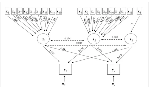
We have fitted a MRBOP model for different values of Q (from 1 to 10) and λ (0.1-10, with increments of 0.10), by using the cross-validation procedure de-scribed in Section 3.2, (training, validation and test sets were 85%, 10%, 5% of the whole sample, respec-tively) and 100 different starting points to avoid local minima. The algorithm converged in 9 iterations lead-ing to the choice of three latent factors (correspond-ing to M SEλ(Q∗=0∗=3).9 = 0.5933), which are weakly
cor-related (0.174, 0.003, 0.244, respectively) as displayed in the path diagram of the estimated model (Figure 3). It turns out that the latent factorz1 is formed by the economical and technical results of the flocks (ex-cept for ECI) together with MOYVET, REMOV, OTH-SPEC, DENSI, VET, strongly correlated to the eco-nomical aspects and it is mainly characterized by the variables DWG, RI and TCI. Latent factorz2 mainly reflects the remaining farming characteristics as biose-curity (through the variable DISINF), surface avail-ability (SURF) and other general features related to the farms as FEED, PAREMPTY, LITTER and ECI (the largest normalized weights are in boldface in Fig-ure 3). Finally, z3 corresponds to one single binary
Setting 1 d= 0.1 d= 1 d= 2
ρwit= 0.90 Model M SEλ∗ L2 MRand %=1 M SEλ∗ L2 MRand %=1 M SEλ∗ L2 MRand %=1
ρbet= 0.10 MRBOP 0.0012 0.0010 1.00 99 0.0012 0.0019 1.00 99 0.0014 0.0046 0.98 95 Ols 0.0012 0.0010 - - 0.0013 0.0028 - - 0.0015 0.0079 - -PCR 0.0033 0.0495 - - 0.0033 0.0499 - - 0.0034 0.0488 - -PLSR 0.0031 0.0442 - - 0.0031 0.0447 - - 0.0031 0.0436 - -ρbet= 0.30 MRBOP 0.0012 0.0011 1.00 99 0.0011 0.0020 1.00 99 0.0012 0.0052 0.97 93 Ols 0.0012 0.0011 - - 0.0012 0.0030 - - 0.0014 0.0089 - -PCR 0.0035 0.0566 - - 0.0036 0.0559 - - 0.0035 0.0562 - -PLSR 0.0032 0.0498 - - 0.0033 0.0490 - - 0.0031 0.0491 - -ρbet= 0.60 MRBOP 0.0006 0.0016 0.96 88 0.0008 0.0031 0.97 94 0.0012 0.0079 0.92 82 Ols 0.0006 0.0010 - - 0.0008 0.0035 - - 0.0013 0.0108 - -PCR 0.0037 0.0719 - - 0.0039 0.0727 - - 0.0040 0.0708 - -PLSR 0.0030 0.0567 - - 0.0033 0.0579 - - 0.0033 0.0562 - -Setting 2 d= 0.1 d= 1 d= 2
ρwit= 0.70 Model M SEλ∗ L2 MRand %=1 M SEλ∗ L2 MRand %=1 M SEλ∗ L2 MRand %=1
ρbet= 0.10 MRBOP 0.0011 0.0015 1.00 98 0.0012 0.0018 1.00 98 0.0012 0.0026 0.96 91 Ols 0.0010 0.0011 - - 0.0012 0.0019 - - 0.0013 0.0038 - -PCR 0.0093 0.0599 - - 0.0098 0.0607 - - 0.0094 0.0592 - -PLSR 0.0063 0.0387 - - 0.0067 0.0392 - - 0.0064 0.0386 - -ρbet= 0.30 MRBOP 0.0010 0.0015 0.98 94 0.0010 0.0019 0.97 92 0.0012 0.0031 0.96 89 Ols 0.0009 0.0012 - - 0.0010 0.0020 - - 0.0014 0.0043 - -PCR 0.0114 0.0715 - - 0.0113 0.0706 - - 0.0117 0.0736 - -PLSR 0.0067 0.0398 - - 0.0066 0.0392 - - 0.0068 0.0409 - -ρbet= 0.60 MRBOP 0.0008 0.0033 0.79 52 0.0009 0.0039 0.82 57 0.0012 0.0051 0.80 55 Ols 0.0004 0.0013 - - 0.0006 0.0023 - - 0.0011 0.0051 - -PCR 0.0191 0.1255 - - 0.0191 0.1238 - - 0.0182 0.1177 - -PLSR 0.0042 0.0258 - - 0.0042 0.0255 - - 0.0044 0.0264 - -Setting 3 d= 0.1 d= 1 d= 2
ρwit= 0.50 Model M SEλ∗ L2 MRand %=1 M SEλ∗ L2 MRand %=1 M SEλ∗ L2 MRand %=1
ρbet= 0.10 MRBOP 0.0014 0.0021 0.97 91 0.0012 0.0021 0.96 89 0.0014 0.0026 0.97 92 Ols 0.0014 0.0018 - - 0.0012 0.0020 - - 0.0016 0.0033 - -PCR 0.209 0.0800 - - 0.0214 0.0821 - - 0.0208 0.0798 - -PLSR 0.0081 0.0284 - - 0.0081 0.0293 - - 0.0080 0.0289 - -ρbet= 0.30 MRBOP 0.0012 0.0024 0.93 84 0.0013 0.0026 0.95 87 0.0016 0.0039 0.92 78 Ols 0.0009 0.0017 - - 0.0012 0.0025 - - 0.0016 0.0040 - -PCR 0.0286 0.1118 - - 0.0283 0.1104 - - 0.0273 0.1050 - -PLSR 0.0070 0.0258 - - 0.0070 0.0256 - - 0.0066 0.0231 - -Setting 4 d= 0.1 d= 1 d= 2
ρwit= 0.30 Model M SEλ∗ L2 MRand %=1 M SEλ∗ L2 MRand %=1 M SEλ∗ L2 MRand %=1
ρbet= 0.10 MRBOP 0.0016 0.0029 0.92 79 0.0016 0.0029 0.91 79 0.0020 0.0037 0.94 83
Ols 0.0014 0.0023 - - 0.0013 0.0024 - - 0.0021 0.0040 -
-PCR 0.0515 0.1420 - - 0.0508 0.1402 - - 0.0484 0.1335 -
-PLSR 0.0064 0.0165 - - 0.0062 0.0162 - - 0.0066 0.0168 -
-Table 2: Simulation results
Fig. 3: Epidemiological data: path diagram
variable (SANPB), representing health problems dur-ing farmdur-ing. Both responses (CONDEMN and MORT) are mainly explained by z1, even though for the car-casses condemnation (CONDEMN) the effect is much stronger (the corresponding coefficients arec11= 7.230 vsc12=−0.381). CONDEMN is also influenced by z3 while MORT byz2. In other words, particular care for the technical performance of the flocks and the health
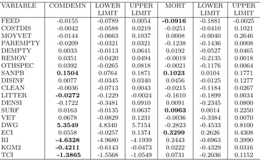
problems during farming should be taken in order to reduce the number of carcasses condemned at slaugh-terhouse. On the other hand, to reduce the mortality (MORT), technical performance and some farm char-acteristics of the flocks need to be improved. Table 4 displays the regression coefficients of the single predic-tors (given by ˆW∗Vˆ∗Cˆ∗) together with the 90% con-fidence intervals computed by a bootstrap procedure
Variables ID Description Y
y1 CONDEMN Percentage of carcasses condemned at slaughterhouse y2 MORT Mortality percentage for the flock
X1
x1 FEED Meat and bone meal-free feeding (1 = yes, 0 = no) x2 COSTDIS Disinfection costs
x3 MOYVET Average veterinary costs for the last three flocks x4 PAREMPTY Partial emptying (1 = yes, 0 = no)
x5 DEMPTY Duration of the empty period before chick arrival x6 REMOV Number of removal to slaughterhouse per flock x7 OTHSPEC Last flock with the same species (1 = yes, 0 = no) x8 SANPB Serious health problem during farming (1 = yes, 0 = no) x9 DISINF Disinfection labour (1 = skilled labour, 0 = yourself) x10 CLEAN Cleaning labour (1 = skilled labour, 0 = yourself) x11 LITTER Quantity of litter used for the flock
x12 DENSI Chick density at the beginning of farming x13 SURF Surface area on which the flock is farmed x14 VET Total amount of veterinary costs for the flock X2
x15 DWG Daily weight gain
x16 ECI Economical consumption index x17 RI Result index
x18 KGM2 Total flock weight slaughtered related to the surface area x19 TCI Technical consumption index
Table 3: Epidemiological data: variable description (Chauvin et al., 2005)
VARIABLE COMDEMN LOWER UPPER MORT LOWER UPPER LIMIT LIMIT LIMIT LIMIT FEED -0.0155 -0.0789 0.0054 -0.0916 -0.1881 -0.0025 COSTDIS -0.0042 -0.0588 0.0219 -0.0251 -0.0410 0.1021 MOYVET -0.0144 -0.0663 0.1037 0.0008 -0.0040 0.2646 PAREMPTY -0.0209 -0.0321 0.0321 -0.1238 -0.1436 0.0008 DEMPTY 0.0033 -0.0113 0.0641 0.0192 -0.0527 0.0465 REMOV 0.0351 -0.0420 0.0494 -0.0019 -0.2135 0.0018 OTHSPEC 0.0392 -0.0265 0.0818 -0.0021 -0.1176 0.0064 SANPB 0.1504 0.0764 0.1871 0.1023 0.0104 0.1771 DISINF 0.0077 -0.0345 0.0340 0.0456 -0.0125 0.1277 CLEAN -0.0036 -0.0713 0.0043 -0.0215 -0.1184 0.0267 LITTER -0.0272 -0.1229 -0.0024 -0.1610 -0.1899 0.0034 DENSI -0.1722 -0.3481 0.0910 0.0091 -0.2345 0.0800 SURF 0.0163 -0.0135 0.0637 0.0963 0.0014 0.2250 VET 0.0678 -0.0829 0.1231 -0.0036 -0.3384 0.0070 DWG 5.3549 4.8340 5.7154 -0.2823 -0.4533 0.8100 ECI 0.0558 -0.0257 0.1374 0.3299 0.2626 0.4308 RI -4.6328 -4.9680 -4.1939 0.2443 -0.6963 0.3990 KGM2 -0.4211 -0.6143 -0.0473 0.0222 -0.4329 0.0316 TCI -1.3865 -1.5568 -1.0549 0.0731 -0.2036 0.1152
Table 4: Epidemiological data: MRBOP regression coefficients and 90% bootstrap confidence intervals
with 1000 bootstrap samples. Looking more in details at the regression coefficient estimates and their corre-sponding confidence intervals, we can observe that the percentage of carcasses condemned at slaughterhouse is influenced mainly by the technical results of the flocks (DWG, RI, TCI, KGM2), presence of health problem (SANPB) and quantity of litter (LITTER). As far as MORT concerns, FEED has a significant negative ef-fect, while ECI, SANPB and SURF have significant positive coefficients. We can conclude that a reduction
of the percentage of carcasses can be achieved mainly by improving technical results of the flocks, while in order to reduce the mortality percentage, some farm-ing (mainly related to sanitary and environmental) fea-tures and economical results of the flocks need to be controlled.
6 Conclusions
In this paper a new model MRBOP for multivariate re-gression based on a small set of weakly correlated latent factors is presented, where each of the latent factors is a linear combination of a subset of correlated predictors. MRBOP is particularly appropriate in a regression con-text where strongly correlated predictors might repre-sent unknown underlying latent dimensions easy to be interpreted. The performance of the proposed approach has been discussed on both simulated and real data sets and generally exhibits accuracy of the estimates and ca-pability to recover the block correlation structure of the original predictors. As suggested by one referee, further developments could extend the linear factor regression based on an “ignoring errors” strategy (since the loss function does not include the error matrix) to an ap-proach able to fit the model with the errors being part of the loss function.
Acknowledgements The authors are grateful to the edi-tor and anonymous referees of Statistics and Computing for their valuable comments and suggestions which improved the clarity and the relevance of the first version.
References
Abdi, H.: Partial least squares regression and projection on latent structure regression (PLS-Regression), Wiley Inter-disciplinary Reviews: Computational Statistics,2, 97–106 (2010)
Abraham, B., Merola, G.: Dimensionality reduction approach to multivariate prediction, Computational Statistics & Data Analysis,48(1), 516 (2005)
Anderson, T.W.: Estimating linear restrictions on regression coefficients for multivariate distributions, Annals of Math-ematical Statistics,22, 327–351 (1951)
Bougeard, S., Hanafi, M., Qannari, E.M.: Multiblock latent root regression. Application to epidemiological data, Com-putational Statistics,22(2), 209–222 (2007)
Bougeard, S., Hanafi, M., Qannari, E.M.: Continuum redundancy-PLS regression: A simple continuum approach, Computational Statistics and Data Analysis,52(7), 3686– 3696 (2008)
Chauvin, C., Buuvrel, I., Belceil, P.A., Orand, J.P., Guille-mot, D., Sanders, P.: A pharmaco-epidemiological analysis of factors associated with antimicrobial consumption level in turkey broiler flocks,36, 199–211 (2005)
De Jong, S.: SIMPLS: an alternative approach to partial least squares regression, Chemometrics and Intelligent Labora-tory Systems,18, 251-263 (1993)
Escoufier, Y.: Le traitement des variables vectorielles, Bio-metrics, 29, 751–760 (1973)
Frank, I.E., Friedman, J.: A statistical view of some chemometrics regression tools, Technometrics,35, 109–148 (1993)
Hocking, R.R.: The Analysis and Selection of Variables in Linear Regression, Biometrics,32, 1–49 (1976)
Hoerl, A.E., Kennard, R.W.: Ridge Regression: Biased Esti-mation for Non-Orthogonal Problems, Technometrics,12, 55–67 (1970)
Hotelling, H.: The most predictable criterion, Journal of Ed-ucational Psychology,25, 139–142 (1935)
Hubert, L., Arabie, P.: Comparing partitions, Journal of Clas-sification,198, 193-218 (1985)
Izenman, A.J.: Reduced-Rank Regression for the Multivariate Linear Model, Journal of Multivariate Analysis,5, 248–262 (1975)
Jolliffe, I.T.: A note on the Use of Principal Components in Regression, Journal of the Royal Statistical Society: Series C (Applied Statistics),31(3), 300–303 (1982)
Krzanowski, W.,J.: Principles of Multivariate Analysis: A User’s Perspective, Oxford University Press, (2000) Rosipal, R., Krmer, N.: Overview and Recent Advances in
Partial Least Squares, In Subspace, Latent Structure and Feature Selection,3940, 34–51 (2006)
Stone, M.: Cross-validation choice and assessment of statisti-cal predictions, Journal of the Royal Statististatisti-cal Society B, 36, 111-147 (1974)
Stone, M., Brooks, R.J.: Continuum Regression: Cross-validated Sequentially Constructed Prediction Embracing Ordinary Least Squares, Partial Least Squares and Princi-pal Components Regression, Journal of the Royal Statisti-cal Society: Series B,52(2), 237–269, (1990)
Tibshirani, R.: Regression shrinkage and selection via the lasso, Journal of the Royal Statistical Society Series B, 58(1), 267–288 (1996)
Tutz, G., Ulbricht, J.: Penalized regression with correlation-based penalty, Statistics and Computing, 19(1), 239–253 (2009)
Van Den Wollenberg, A.L.: Redundancy analysis an alter-native for canonical correlation analysis, Psychometrika, 42(2), 207–219 (1977)
Waldro, L., Pintilie, M., Tsao, M.S., Shepherd, F.A., Hutten-hower, C., Jurisica, I.: Optimized application of penalized regression methods to diverse genomic data, Bioinformat-ics,27(24), 3399–3406 (2011)
Witten, D.M., Tibshirani, R.: Covariance-regularized regres-sion and classification for high dimenregres-sional problems, Jour-nal of the Royal Statistical Society: Series B (Statistical Methodology),71, 615–636 (2009)
Wold, H.: Estimation of principal components and related models by iterative least squares, In: P.R. Krishnaiaah (Ed.), Multivariate Analysis, New York, 391–420 (1966) Yuan, M., Ekici, A., Lu, Z., Monteiro, R.: Dimension
reduc-tion and coefficient estimareduc-tion in multivariate linear re-gression, Journal of the Royal Statistical Society: Series B (Statistical Methodology),69, 329–346 (2007)
Yuan, M., Lin, Y.: Model selection and estimation in regres-sion with grouped variables, Journal of the Royal Statisti-cal Society: Series B,68, 49–67 (2006)
Zou, H., Hastie, T.: Regularization and variable selection via the elastic net, Journal of the Royal Statistical Society Se-ries B,67, 301–320 (2005)