An Ensemble of Optimal Trees for Classification and Regression (OTE)

(1)

An Ensemble of Optimal Trees for Classification and

Regression (

OTE

₎

Zardad Khana,b,∗, Asma Gulb,c, Aris Perperogloub, Miftahuddin Miftahuddinb,f, Osama Mahmoudb,d, Werner Adlere, Berthold Lausenb,∗∗,

a_{Department of Statistics, Abdul Wali Khan University, Mardan, Pakistan} b_{Department of Mathematical Sciences, University of Essex, Colchester CO4 3SQ, UK}

c_{Department of Statististics, Shaheed Benazir Bhutto Women University Peshawar,}

Pakistan

d_{School of Oral & Dental Sciences, University of Bristol, UK}

e_{Department of Biometry and Epidemiology, University of Erlangen-Nuremberg, Germany} f_{College of Science, Syiah Kuala University - Banda Aceh, Indonesia}

Abstract

Predictive performance of a random forest ensemble is highly associated with the strength of individual trees and their diversity. Ensemble of a small number of accurate and diverse trees, if prediction accuracy is not compromised, will also reduce computational burden. We investigate the idea of integrating trees that are accurate and diverse. For this purpose, we utilize out-of-bag observation as validation sample from the training bootstrap samples to choose the best trees based on their individual performance and then assess these trees for diversity using Brier score. Starting from the first best tree, a tree is selected for the final ensemble if its addition to the forest reduces error of the trees that have already been added. A total of 35 bench mark problems on classification and regression are used to assess the performance of the proposed method and compare it withkNN, tree, random forest, node harvest and support vector machine. We compute unexplained variances and classification error rates for all the methods on the corresponding data sets. Our experiments reveal that the size of the ensemble is reduced significantly and better results are obtained in most of the cases. For further verification, a simulation study is also given where four tree

∗_{[email protected]}

(2)

style scenarios are considered to generate data sets with several structures.

Keywords: classification and regression trees, random forest, ensemble methods, accuracy and diversity.

1. Introduction

Many studies have suggested that combining weak models leads to eﬃcient ensembles [1, 2, 3, 4, 5, 6, 7] that are used frequently in many real world problems[8, 9, 10, 11]. Combining the outputs of multiple classifiers also re-duces generalization error [2, 3, 12, 4]. Ensemble methods are eﬀective in that

5

diﬀerent types of models have diﬀerent inductive biases where such diversity reduces variance-error while not increasing the bias error [13, 14, 15].

Extending this notion, Breiman [16] suggested growing a large number, T for instance, of classification and regression trees. Trees are grown on bootstrap samples form a given training dataL= (X,Y) ={(x1, y1),(x2, y2), ...,(xn, yn)}.

10

Thexiare observations ondfeatures andyvalues are from real line and a set of

known classes (1,2,3, ..., K) in cases of regression and classification, respectively. Breiman called this method as random forest.

As the number of trees in random forest is often very large, there has been a significant work done on the problem of minimizing this number to reduce

15

computational cost without decreasing prediction accuracy[17, 18, 19, 20]. Overall prediction error of a random forest is highly associated with the strength of individual trees and their diversity in the forest. This idea is backed by Breiman’s[16] upper bound for the overall prediction error of random forest given by

20

!

Err≤ρ¯err_"j, (1)

where j = 1,2,3, ..., T, T denotes the number of all trees, Err! is the overall prediction error of the forest, ¯ρrepresents weighted correlation between residuals from two independent trees and err_"j is the prediction error of thejth tree in

(3)

Based on the above discussion, this article proposes to select the best trees,in

25

terms individual accuracy and diversity, from a large ensemble grown by random forest. Using 35 benchmark data sets, the results from the new method are compared with those of kNN, tree classifier, random forest, node harvest and support vector machine. For further verification, a simulation study is also given where data sets with many tree structures are generated. The rest of the paper

30

is organized as follows. The proposed method and the underlying algorithm are given in section 2, experiments and results based on benchmark and simulated data sets are given in section 3. Finally, section 4 gives the conclusion of the paper.

2. OTE: Optimal Trees Ensemble 35

Random forest refines bagging by introducing additional randomness in the base models, trees, by drawing subsets of the predictor set for partitioning the nodes of a tree[4] . This article investigates the possibility of further refine-ment by proposing the method of trees selection on the basis of their individ-ual accuracy and diversity using unexplained variance and Brier score [21] in

40

cases of regression and classification respectively. To this end, we partition the given training data L = (X,Y) randomly into two non overlapping portions,

LB= (XB,YB) andLV= (XV,YV). GrowT classification or regression trees

onT bootstrap samples from the first portion LB = (XB,YB). While doing

so, select a random sample ofp < dfeatures from the entire set ofdpredictors.

45

This inculcates additional randomness in the trees. Due to bootstraping, there will be some observations left out of the samples which are called out-of-bag (OOB) observations. These observations take no part in the training of tree. These observatons can be utilized in two ways:

1. In case of regression, out-of-bag observations are used to estimate

unex-50

plained variances of each tree grown on a bootstrap sample. Trees are then ranked in ascending order whith respect to their unexplained vari-ances and the top rankedM trees are chosen.

(4)

2. In case of classification, out-of-bag observations are used to estimate error rates of the trees. Trees are then ranked in ascending order whith respect

55

to their error rates and the top rankedM trees are chosen. A diversity check is carried out as follows

1. Starting from the two top ranked trees, successive ranked trees are added one by one to see how they perform on the independent validation data,

LV = (XV,YV). This is done until the lastMth tree is added. 60

2. Select tree ˆLk, k = 1,2,3, ..., M if its inclusion to the ensemble without

the kth tree satisfys the following two criteria given for regression and classification respectively.

(a) In regression case, letU.EX P⟨−k⟩be the unexplained variance of the ensemble not having thekth tree andU._{EX P}⟨+k⟩be the unexplained

65

variance of the ensemble withkth tree included, then tree ˆLkis chosen

if

U.EX P⟨+k⟩

<U.EX P⟨−k⟩ .

(b) In classification case, let ˆBS⟨−k⟩ be the Brier score of the ensemble not having thekth tree and ˆBS⟨+k⟩be the Brier score of the ensemble withkth tree included, then tree ˆLk is chosen if

70 ˆ BS⟨+k⟩<BSˆ ⟨−k⟩, where ˆ BS= ## of test cases i=1 $ yi−Pˆ(yi|X) %2

total # of test instances ,

yi is the state ofyi for observationiin the (0,1) form and ˆP(y|X) is

the binary response probability estimate given the features.

These trees, named as optimal trees, are then combined and are allowed to vote, in case of classification, or average, in case of regression, for new/test data. The

75

(5)

2.1. The Algorithm

Steps of the proposed algorithm both for regression and classification are 1. Take T bootstrap samples from the given portion of the training data

LB= (XB,YB).

80

2. Grow regression/classification trees on all the bootstrap samples using random forest technique.

3. ChooseM trees with the smallest individual prediction error on the train-ing data.

4. Add theM selected trees one by one and select a tree if it improves

per-85

formance on validation data,LV= (XV,YV), using unexplained variance

and Brier score in cases of regression and classification as the respective performance measures.

5. Combine and allow the trees to vote, in case of classification, or average, in case of regression, for new/test data.

90

An illustrative flow chart of the proposed algorithm can be seen in Figure 1. An algorithm based on a similar idea has previously been proposed where instead of classification and regression trees, probability estimation trees are used [22]. The ensemble of probability estimation trees is used for estimating class membership probabilities in binary class problems. Ensembles selection for

95

kNN classifiers have also been proposed recently where in addition to individual accuracy, thekNN models are grown on random subsets of the feature set instead of considering the entire space [23, 24].

3. Experiments and Results 3.1. Simulation

100

This section presents four simulation scenarios each consisting of various tree structures. The aim is to make the recognition problem slightly diﬃcult for classifiers likekNN and CART, and to provide a challenging task for the most complex method like SVMs and random forest. In each of the scenarios, four

(6)

(7)

diﬀerent complexity levels are considered by changing the weightsηijkof the tree

105

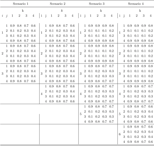
nodes. Consequently, four diﬀerent values of the Bayes error are obtained where the lowest Bayes error indicates a data set with meaningful patterns and the highest Bayes error means a data set with no patterns. Table 1 gives various values of ηijk used in Scenarios 1, 2, 3, and 4. Node weights for obtaining

the complexity levels are listed in four columns of the table fork = 1,2,3,4,

110

for each model. A generic equation for producing class probabilities of the bernoulli responseY= Bernoulli(p) given then_×3T dimensional vectorXof n iidobservations from Uniform(0,1) is.

p(y|X) = exp

&

c2×&Zm

T −c1

''

1 +exp&c2×&Zm

T −c1 '', whereZm= T ( t=1 ˆ pt. (2)

c1 and c2 are some arbitrary constants, m = 1,2,3,4 is scenario number and

Zm’s aren×1 probability vectors. T is the total number of trees used in a

115

scenario and ˆpt’s are class probabilities for a particular response in Y. These

probabilities are generated by the following tree structures ˆ

p1 = η11k×1(x1≤0.5&x3≤0.5)+η12k×1(x1≤0.5&x3>0.5)+η13k×1(x1>0.5&x2≤0.5)

+η14k×1(x1>0.5&x2>0.5), ˆ

p2 = η21k×1(x4≤0.5&x6≤0.5)+η22k×1(x4≤0.5&x6>0.5)+η23k×1(x4>0.5&x5≤0.5) +η24k×1(x4>0.5&x5>0.5),

ˆ

(8)

where 0<ηijk<1 are weights given to to the nodes of the trees,k= 1,2,3,4.

The four scenarios use the following specifications for using (2)

3.1.1. Scenario 1 120

This scenario consists of 3 tree components each grown on 3 variables which follows that,T = 3,Z1=#3t=1pˆt andXbecomes an×9 dimensional vector.

3.1.2. Scenario 2

In this scenario we take a total ofT = 4 trees whereZ2=#4t=1pˆtsuch that

Xbecomes an×12 dimensional vector.

125

3.1.3. Scenario 3

This scenario is based onT = 5 trees such thatZ3=#5t=1pˆtandXbecomes

an×15 dimensional vector.

3.1.4. Scenario 4

This scenario consists of 6 tree components which follows that,T = 6,Z4= 130

#6

t=1pˆtandXbecomes an×18 dimensional vector.

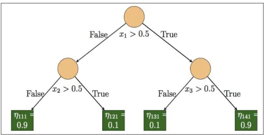
To understand how the trees are grown in the above simulation scenarios, a tree used in simulation Scenario 1.1 is given in Figure 2.

(9)

Table 1: Node weights,ηijk, used in simulation scenarios wherei is tree number,jis node

number in each tree andkis denoting a variant of the weights for the four complexity levels

for all the scenarios.

Scenario 1 Scenario 2 Scenario 3 Scenario 4

k k k k i j 1 2 3 4 i j 1 2 3 4 i j 1 2 3 4 i j 1 2 3 4 1 1 0.9 0.8 0.7 0.6 1 1 0.9 0.8 0.7 0.6 1 1 0.9 0.9 0.9 0.8 1 1 0.9 0.9 0.9 0.8 2 0.1 0.2 0.3 0.4 2 0.1 0.2 0.3 0.4 2 0.1 0.1 0.1 0.2 2 0.1 0.1 0.1 0.2 3 0.1 0.2 0.3 0.4 3 0.1 0.2 0.3 0.4 3 0.1 0.1 0.1 0.2 3 0.1 0.1 0.1 0.2 4 0.9 0.8 0.7 0.6 4 0.9 0.8 0.7 0.6 4 0.9 0.9 0.9 0.8 4 0.9 0.9 0.9 0.8 2 1 0.9 0.8 0.7 0.6 2 1 0.9 0.8 0.7 0.6 2 1 0.9 0.9 0.9 0.8 2 1 0.9 0.9 0.9 0.8 2 0.1 0.2 0.3 0.4 2 0.1 0.2 0.3 0.4 2 0.1 0.1 0.1 0.2 2 0.1 0.1 0.1 0.2 3 0.1 0.2 0.3 0.4 3 0.1 0.2 0.3 0.4 3 0.1 0.1 0.1 0.2 3 0.1 0.1 0.1 0.2 4 0.9 0.8 0.7 0.6 4 0.9 0.8 0.7 0.6 4 0.9 0.9 0.9 0.8 4 0.9 0.9 0.9 0.8 3 1 0.9 0.8 0.7 0.6 3 1 0.9 0.8 0.7 0.6 3 1 0.9 0.8 0.7 0.7 3 1 0.9 0.9 0.9 0.8 2 0.1 0.2 0.3 0.4 2 0.1 0.2 0.3 0.4 2 0.1 0.2 0.3 0.3 2 0.1 0.1 0.1 0.2 3 0.1 0.2 0.3 0.4 3 0.1 0.2 0.3 0.4 3 0.1 0.2 0.3 0.3 3 0.1 0.1 0.1 0.2 4 0.9 0.8 0.7 0.6 4 0.9 0.8 0.7 0.6 4 0.9 0.8 0.7 0.7 4 0.9 0.9 0.9 0.8 4 1 0.9 0.8 0.7 0.6 4 1 0.9 0.8 0.7 0.7 4 1 0.9 0.8 0.7 0.7 2 0.1 0.2 0.3 0.4 2 0.1 0.2 0.3 0.3 2 0.1 0.2 0.3 0.3 3 0.1 0.2 0.3 0.4 3 0.1 0.2 0.3 0.3 3 0.1 0.2 0.3 0.3 4 0.9 0.8 0.7 0.6 4 0.9 0.8 0.7 0.7 4 0.9 0.8 0.7 0.7 5 1 0.9 0.8 0.7 0.7 5 1 0.9 0.8 0.7 0.6 2 0.1 0.2 0.3 0.3 2 0.1 0.2 0.3 0.4 3 0.1 0.2 0.3 0.3 3 0.1 0.2 0.3 0.4 4 0.9 0.8 0.7 0.7 4 0.9 0.8 0.7 0.6 6 1 0.9 0.8 0.7 0.6 2 0.1 0.2 0.3 0.4 3 0.1 0.2 0.3 0.4 4 0.9 0.8 0.7 0.6

(10)

Ta b le 2 : C la ss ifi ca ti o n er ro r (i n % a g e) o f k NN, tr ee , ra n d o m fo re st , n o d e h a rv est , S VM a n d O T E . T h e fo rt h co lu m n o f th e ta b le sh ow s B ay es er ro r fo r ea ch m o d el . T h e la st co lu m n is th e p erc en ta g e re d u ct io n int h e si ze o f OT E co m p a red to ra n d o m fo res t Mo de l dn B ay es k N N T re e R F N H S V M S V M S V M S V M O T E R ed u ct io n in E rr o r (R a d ia l) (L in ea r) (B es se l) (L a p la cia n ) E n se m b le S iz e (% ) 9 .0 2 2 9 .9 9 .6 9 .8 1 9 1 9 1 9 1 9 9 .5 9 1 14 26 15 15 15 22 22 23 22 15 90 S ce n a rio 1 9 1 0 0 0 1 7 3 2 1 8 1 8 2 1 2 8 2 8 2 8 2 8 1 8 9 0 33 42 36 35 36 37 37 38 37 37 91 21 29 22 21 21 24 23 30 24 21 90 24 31 25 24 24 26 26 32 26 23 90 S ce n a rio 2 1 2 1 0 0 0 2 8 3 6 3 0 2 8 2 9 3 1 3 0 3 6 3 1 2 9 9 0 30 39 32 32 32 33 33 38 33 32 89 15 31 22 18 22 24 24 55 24 18 91 18 32 24 21 24 26 25 55 26 22 89 S ce n a rio 3 1 5 1 0 0 0 2 1 3 4 2 5 2 3 2 7 2 7 2 7 5 5 2 7 2 4 9 1 24 36 29 28 29 29 29 54 30 28 90 21 34 28 23 25 25 25 72 27 22 90 22 35 27 23 26 27 27 71 28 24 89 S ce n a rio 4 1 8 1 0 0 0 2 5 3 9 3 1 2 6 2 9 3 1 3 1 6 7 3 5 2 7 9 0 26 40 31 28 30 32 32 68 36 29 90

(11)

The values ofc1 and c2 are fixed at 0.5 and 15, respectively, in all the sce-narios for all variants. A total ofn= 1000 observation are generated using the

135

above setup. kNN, CART, random forest, node harvest, SVM and OTE are trained by using 90% of the data as training data (of which 90% is for bootstring and 10% for diversity check, in the case ofOTE) and then applying the remain-ing 10% data as test data for testremain-ing purpose. A total of 1000 realizations are made under each scenario. The results obtained in all the scenarios are given in

140

Table 2. Node weights are changed in a manner that could make the patterns in the data less meaningful and thus getting a higher Bayes error. This can be observed in the fourth column of Table 2, where each scenario has four diﬀerent values of the Bayes error. As anticipated, kNN and tree classifiers have the highest percentage errors in all the four scenarios. Random forest and OTE 145

performed quite similarly with slight variations in few cases. In cases where the models have the highest Bayes error, the results of random forest are better or comparable with those ofOTE. In all the remaing cases where the Bayes error is the smallest,OTE is better or comparable with random forest. SVM performed very similarly tokNN and tree. Percentage reduction in ensemble size ofOTE 150

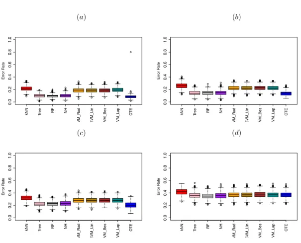
is also shown in the last column of the table. This follows thatOTE could be very helpful in decreasing the size of the ensemble thus reducing storage costs. The box plots given in Figure 3 reveal that the best results of OTE can be observed in Figure (a) where a data set with meaningful tree structures is generated. Figure (d) is the worst example of OTE where the Bayes error is

155

the highest (i.e. 33%), and where the data have no meaningful tree structures.

3.2. Benchmark Problems

For assessing the performance of OTE on benchmark problems, we have considered 35 data sets out of which 14 are regression and 21 classification problems. A brief summary of the data sets is given in Table 3. The upper

160

portion of table 3 is a summary of regression problems whereas the lower portion is a summary of classification problems.

(12)

Table 3: Data sets for classification and regression with total number of observations n,

number of featuresdand feature type; F: real, I: integer and N: nominal features in a data

set. Sources are also given.

Data Set n d Feature type Source

(R/I/N) Regression Bone 485 3 (1/1/1) [25, 26] Galaxy 323 4 (4/0/0) [25, 27] Friedman 1200 5 (5/0/0) [28] CPU 209 7 (7/0/0) [29] Concrete 103 7 (7/0/0) [29] Abalone 4177 8 (7/0/1) [29] MPG 398 8 (2/2/4) [29] Stock 950 9 (9/0/0) http://funapp.cs.bilkent.edu.tr/DataSets/ Wine 1599 11 (11/0/0) [29] Ozone 203 12 (9/0/3) [30] Housing 506 13 (12/0/1) [31] Pollution 60 15 (7/8/0) http://openml.org/ Treasury 1049 15 (15/0/0) http://sci2s.ugr.es/keel/dataset.php?cod=42 Baseball 337 16 (2/14/0) http://sci2s.ugr.es/keel/dataset.php?cod=76#sub2 Classification Mammographic 830 5 (0/5/0) http://sci2s.ugr.es/keel/category.php?cat=clas Dystrophy 209 5 (2/3/0) [32] Monk3 122 6 (0/6/0) [29] Appendicitis 106 7 (7/0/0) http://sci2s.ugr.es/keel/dataset.php?cod=183 SAHeart 462 9 (5/3/1) http://sci2s.ugr.es/keel/dataset.php?cod=184#sub1 Tic-Tac-Toe 958 9 (0/0/9) [29] Heart 303 13 (1/12/0) [29] House vote 232 16 (0/0/16) [29] Bands 365 19 (13/6/0) http://sci2s.ugr.es/keel/dataset.php?cod=184#sub1 Hepatitis 80 20 (2/18/0) [29] Parkinson 195 22 (22/0/0) [29] Body 507 23 (22/1/0) [33] Thyroid 9172 27 (3/2/22) [29] WDBC 569 29 (29/0/0) [29] WPBC 198 32 (30/2/0) [29] Oil-Spill 937 49 (40/9/0) http://openml.org/ Spam base 4601 57 (55/2/0) [29] Glaucoma 196 62 (62/0/0) [32] Nki 70 144 76 (71/5/0) [34] 12

(13)

(a) (b) 0.0 0.2 0.4 0.6 0.8 1.0 Error Rate kNN Tree RF NH

SVM_Rad SVM_Lin SVM_Bes SVM_Lap

O TE 0.0 0.2 0.4 0.6 0.8 1.0 Error Rate kNN Tree RF NH

O TE (c) (d) 0.0 0.2 0.4 0.6 0.8 1.0 Error Rate kNN Tree RF NH

O TE 0.0 0.2 0.4 0.6 0.8 1.0 Error Rate kNN Tree RF NH

O

TE

Figure 3: Box plots forkNN, tree, random forest (RF), node harvest (NH), SVM and (OTE)

on the data simulated in Scenario 1. (a): simulation with Bayes error 9%, (b): simulation with Bayes error 14%, (c): simulation with Bayes error 17% and (d): simulation with Bayes

error 33%. The best results ofOTE can be seen in fugure (a) where the model produces a

data with almost perfect tree structures. Figure (d) is the worst example ofOTE

3.3. Experimental Setup for Benchmark Data Sets

Experiments carried out on the 35 data set are designed as follows. Each data set is divided into two parts, a training part and testing part. The training

165

part consists of 90% of the total data while the testing part consists of the remaining 10% of the data. A total of T = 1500 independent classification and regression trees are grown on bootstrap samples from the (90% of) training data along with randomly selectingpfeatures for splitting the nodes of the trees. The remaining 10% of training data is used for diversity check. In the cases of

(14)

both regression and classification, the numberpof features is kept constant at p=)(d) for all data sets. The best of the totalT trees are selected by using the method given in Section 2 and are used as the final ensemble (M is taken as 20% ofT). Testing part of the data is applied on the final ensemble and a total of 1000 runs are carried out for each data set. Final result is the average

175

of all these 1000 runs.

For tuning various parameters of CART, we used the R-Function “tune.rpart” available within the R-Package “e1071”. We tried various values, (5,10,15,20,25,30) for finding the optimal number of splits and the minimal optimal depth of the trees.

180

For tuning the hyper parameters,nodesize, ntree and mtry of random for-est, we used the function “tune.randomForest” available with in the R-Package “e1071” as used by [36]. For tuning the node size we tried values (1,5,10,15,20,25,30), for tuning ntree we tried values (500,1000,1500,2000) and for tuning mtry, we tried (sqrt(d), d/5, d/4, d/3, d/2). We tried all the possible values of mrty

185

whered <12.

The only parameter in the node harvest estimator is the number of nodes in the initial ensemble and for its large values the results are insensitive [18]. Meinshausen [18] showed for various data sets that initial ensemble size greater than 1000 yields almost the same results. In our experiments we kept this value

190

fixed at 1500. In case of SVM, automatic estimation of sigma was used available with in the R package “kernlab”. The rest of the parameters are kept at default values.

The same set of training and test data is used for tree, random forest, node harvest, SVM and our proposed method. Average unexplained variances and

195

classification errors, for regression and classification respectively, are noted down for all the four methods on the data sets. All the experiments are done using R-Program version 3.0.2 [37]. The results are given in tables 4 and 5 for regression and classification respectively.

(15)

b le 4 : U n ex p la in ed va ri a n ce s fo r re g re ss io n d a ta se ts fr o m k NN, tr ee , ra n d o m fo re st , n o d e h a rv est , S VM a n d OT E .T h e u n ex p la in ed va ri a n ce o f e b es t p er fo rm in g m eth o d fo r th e co rr es p o n d in g d a ta se t is sh ow n in b o ld . Da ta S et nd k NN T re e R F NH S VM S VM S VM S VM O T E (R a d ia l) (L in ea r) (B es se l) (L a p la cia n ) B o n e 4 8 5 3 0 .8 9 3 2 0 .7 0 5 8 0 .6 6 0 1 0 .6 6 3 2 0. 6292 0 .7 9 0 8 0 .7 3 6 9 0 .6 3 2 9 0 .6 4 5 4 G a la x y 3 2 3 4 0 .0 2 8 5 0 .0 9 5 2 0 .0 2 7 5 0 .0 6 8 6 0. 0253 0 .1 1 5 3 0 .0 3 5 6 0 .0 2 6 2 0 .0 2 6 1 F rie d m a n 1 2 0 0 5 0 .1 3 7 3 0 .3 8 7 1 0 .1 2 1 2 0 .4 4 5 2 0. 0559 0 .2 8 2 8 0 .0 8 4 9 0 .0 6 5 7 0 .1 3 6 4 C P U 2 0 9 7 0 .1 0 5 8 0 .2 8 3 8 0 .0 6 4 6 0 .2 6 5 9 0 .3 8 9 8 0 .0 9 1 6 0 .2 8 6 1 0 .3 1 4 3 0. 0600 C o n cr et e 1 0 3 7 0 .3 7 2 0 0 .4 9 8 9 0 .2 1 7 4 0 .4 3 0 7 0 .0 7 0 0 0 .1 7 4 3 0. 0623 0 .1 8 0 6 0 .2 3 4 2 A b a lo n e 4 1 7 7 8 0 .5 3 4 7 0 .5 6 7 3 0. 4386 0 .6 0 8 3 0 .4 4 1 0 0 .4 9 0 4 0 .4 4 3 3 0 .4 4 1 8 0 .4 4 7 3 M P G 3 9 8 8 0 .3 2 3 0 0 .2 3 0 1 0 .1 2 5 9 0 .1 9 9 0 0 .1 3 5 8 0 .2 0 6 6 0 .1 4 3 5 0 .1 3 5 9 0. 1203 St o ck 9 5 0 9 0. 0102 0 .0 9 4 2 0 .0 1 2 1 0 .1 1 9 2 0 .0 1 5 3 0 .1 3 7 3 0 .0 2 7 4 0 .0 1 4 2 0 .0 1 1 0 W in e 1 5 9 9 1 1 0 .8 9 7 5 0 .7 1 4 0 0. 4933 0 .7 0 4 4 0 .5 9 8 0 0 .6 6 5 3 0 .8 9 9 1 0 .5 8 5 9 0 .5 0 7 2 O zo n e 2 0 3 1 2 0 .6 4 3 0 0 .4 3 6 6 0 .3 0 6 1 0 .3 6 4 2 0. 2488 0 .3 5 2 8 0 .7 9 6 7 0 .2 7 5 0 0 .3 0 1 6 H o u sin g 5 0 6 1 3 0 .4 6 9 6 0 .2 8 2 1 0 .1 1 9 0 0 .2 4 7 7 0 .1 7 5 6 0 .3 0 5 5 0 .8 8 2 4 0 .1 8 5 3 0. 1160 P o llu tio n 6 0 1 5 0 .9 5 0 0 0 .9 5 0 0 0 .6 7 7 9 0 .7 7 2 8 0 .6 9 4 2 0 .8 1 4 4 0 .9 5 0 0 0 .7 3 2 6 0. 6653 T re a su ry 1 0 4 9 1 5 0 .0 0 7 5 0 .0 4 0 5 0 .0 0 4 0 0 .0 5 7 4 0 .0 0 6 2 0 .0 0 6 0 0 .0 0 7 7 0 .0 070 0. 0039 B a se b a ll 3 3 7 1 6 0 .6 9 3 1 0 .3 5 1 3 0 .3 4 3 4 0 .3 9 0 8 0 .3 6 4 1 0 .3 8 1 8 0 .8 7 6 5 0 .3 6 4 1 0. 3329

(16)

Ta b le 5 : C la ss ifi ca ti o n er ro r ra te s o f k NN, tr ee , ra n d o m fo re st , n o d e h a rv est , S VM a n d OT E .T h e re su lt o f th e b es t p er fo rm in g m et h o d fo r th e co rr es p o n d in g d a ta set is sh ow n in b o ld . Da ta S et nd k NN T re e R F NH S VM S VM S VM S VM O T E (R a d ia l) (L in ea r) (B es se l) (L a p la cia n ) M a m m o g ra p h ic 8 3 0 5 0 .1 9 0 1 0 .1 6 3 1 0 .1 6 7 0 0. 1579 0 .1 9 1 0 0 .1 7 5 0 0 .1 8 7 5 0 .1 8 6 3 0 .1 7 1 1 D y st ro p h y 2 0 9 5 0 .1 1 7 2 0 .1 4 8 2 0 .1 1 5 4 0 .1 4 7 0 0 .0 9 9 9 0 .1 1 2 2 0 .1 0 7 0 0. 0997 0 .1 1 8 2 M o n k 3 1 2 2 6 0 .1 2 2 6 0 .0 7 7 3 0. 0728 0 .2 6 9 9 0 .0 9 5 3 0 .2 2 5 4 0 .0 9 2 8 0 .0 9 3 8 0 .0 7 3 1 A p p en d ic it is 1 0 6 7 0 .1 4 2 3 0 .1 6 4 0 0 .1 4 5 5 0. 1380 0 .2 2 4 5 0 .1 7 2 6 0 .1 9 0 5 0 .1 6 5 0 0 .1 5 0 0 S A H ea rt 4 6 2 9 0 .3 3 6 3 0 .2 9 1 1 0 .2 8 9 7 0. 2762 0 .3 0 7 5 0 .3 0 8 0 0 .3 3 3 2 0 .3 1 3 9 0 .3 1 7 8 T ic -T a c-T o e 9 5 8 9 0 .3 6 1 7 0 .1 0 8 2 0. 0317 0 .2 8 6 1 0 .2 0 7 8 0 .3 9 4 8 0 .1 7 2 5 0 .1 9 7 2 0 .0 3 5 3 H ea rt 3 0 3 1 3 0 .3 5 0 0 0 .2 1 0 8 0 .1 6 2 9 0 .1 8 9 2 0 .2 3 4 2 0 .1 7 4 5 0. 1612 0 .1 7 1 9 0 .1 7 4 3 H o u se V o te 2 3 2 1 6 0 .0 8 2 5 0 .0 3 4 5 0. 0322 0 .1 0 2 0 0 .0 3 3 0 0 .0 4 7 0 0 .2 2 1 1 0 .0 5 2 9 0 .0 3 4 0 B a n d s 3 6 5 1 9 0 .3 1 9 6 0 .3 6 8 3 0 .2 6 8 3 0 .3 6 4 7 0 .3 6 6 9 0 .3 2 0 2 0 .4 7 2 4 0 .5 5 7 3 0. 2601 H ep a tit is 8 0 2 0 0 .3 8 3 1 0 .1 8 6 8 0 .1 3 8 5 0 .1 2 9 6 0 .1 4 0 6 0 .1 5 6 8 0 .5 6 2 9 0 .1 4 9 0 0. 1229 P a rk in so n 1 9 5 2 2 0 .1 6 2 0 0 .1 4 5 6 0 .0 8 9 4 0 .1 2 3 5 0 .1 3 8 5 0 .1 9 4 1 0 .2 8 3 8 0 .1 9 28 0. 0859 B o d y 5 0 7 2 3 0 .0 2 2 6 0 .0 7 8 8 0 .0 3 9 5 0 .0 7 4 4 0 .0 1 5 6 0. 0136 0 .5 5 0 5 0 .0 2 1 9 0 .0 3 8 0 T h y ro id 9 1 7 2 2 7 0 .0 3 8 8 0 .0 1 2 6 0. 0100 0 .0 2 0 3 0 .1 1 1 3 0 .0 3 1 0 0 .2 9 3 6 0 .0 8 3 4 0. 0100 W D B C 5 6 9 2 9 0 .0 6 7 1 0 .0 6 8 6 0 .0 3 8 8 0 .0 5 2 5 0 .0 4 1 5 0. 0264 0 .6 2 9 7 0 .0 4 0 3 0 .0 3 7 5 W P B C 1 9 8 3 2 0 .2 4 1 3 0 .2 8 1 5 0 .1 9 5 8 0 .2 2 8 2 0 .2 8 4 8 0 .2 8 8 1 0 .5 6 8 4 0 .3 0 8 4 0. 1921 O il-S p ill 9 3 7 4 9 0 .0 4 3 5 0 .0 3 6 6 0 .0 3 3 0 0 .0 3 6 0 0 .0 7 5 6 0 .1 4 0 0 0 .0 3 8 7 0 .1 4 6 7 0. 0321 S p a m b a se 4 6 0 1 5 8 0 .1 7 4 7 0 .1 0 8 3 0 .0 4 6 9 0 .0 9 4 4 0 .0 9 4 1 0 .0 7 2 5 0 .4 8 2 0 0 .1 020 0. 0460 S o n a r 2 0 8 6 0 0 .1 7 9 0 0 .2 8 7 9 0 .1 6 1 5 0 .2 3 9 0 0 .1 7 1 0 0 .2 5 0 5 0 .5 3 0 0 0 .2 6 9 8 0. 1600 G la u co m a 1 9 6 6 2 0 .1 9 3 4 0 .1 2 3 7 0 .1 0 5 2 0 .1 1 5 4 0 .1 1 0 8 0 .1 5 6 5 0 .6 3 9 7 0 .1 6 6 4 0. 1051 N k i 7 0 1 4 4 7 6 0 .1 8 2 7 0 .1 6 8 3 0 .1 4 6 6 0 .1 4 4 8 0 .2 6 6 4 0 .3 3 8 1 0 .4 2 6 0 0 .4 0 8 9 0. 1399 M u sk 4 7 6 1 6 6 0 .1 4 2 0 0 .2 2 5 6 0 .1 1 0 3 0 .2 4 4 4 0 .1 3 2 6 0 .1 4 4 0 0 .4 9 6 4 0 .4 6 9 8 0. 0949

(17)

3.4. Discussion 200

The results given in tables 4 and 5 show that the proposed method is per-forming better than the other methods on many of the data sets. In the case of regression problems, our method is giving better results than the other methods considered on 7 data sets out of a total of 14 data sets, whereas on 2 data sets, Wine and Abalone, random forest gives the best performance. On 5 of the data

205

sets, Bone, Galaxy, Freidman, and Ozone, SVM with radial kernel and Concrete with Bessel kernel gave the best results. Tree andkNN are unsurprisingly the worst performers in all the methods with the exception of Stock data set where kNN is the best.

In the case of classification problems, the new method is giving better results

210

than the other methods considered on 10 data sets out of a total of 21 data sets and comparable to random forest on 1 data set. On 3 data sets, random forest gives the best performance. On three of the data sets, Mammographic, Appendicitis and SAHeart, node harvest classifier gives the best result among all other methods. SVM is better than the others on 4 data sets.

215

Overall, the proposed method gave better results on 15 data sets and com-parable results on 2 data set.

We kept all our parameters in the ensemble fixed for the sake of simplicity. Searching for the optimal total number T of trees grown before the selection process, the percentageM of best trees selected at the first phase, node size

220

and the number of features for splitting the nodes might further improve our results. Large values are recommended for the size of the initial set under the available computation resources and a value of T ≥ 1500 is expected to work well in general. This can be seen in Figure 4 that show the eﬀect of the number of trees in the initial set on (a): unexplained variance and (b): misclassification

225

error for the data sets given usingOTE.

One important parameter of the our method is the number M of best trees selected at the first phase for the final ensemble. Various values of M reveal diﬀerent behaviour of the method. We considered the eﬀect of M =

(18)

(a) (b) 0 1000 2000 3000 4000 0.0 0.2 0.4 0.6 0.8 1.0

Number of Trees in Initial Set

Une xplained V ar iance Bone Galaxy Stock Ozone Housing Baseball 0 1000 2000 3000 4000 0.0 0.1 0.2 0.3 0.4

Number of Trees in Initial Set

Error Rate Hepatitis Body Thyroid WDBC WPBC Glaucoma

Figure 4: The eﬀect of the number of trees in the initial set on (a): unexplained variance and

(b): misclassification error for the data sets given usingOTE. In both the cases, number of

trees larger than 1500 can be recommended

(a) (b) 0 10 20 30 40 50 60 70 0.0 0.1 0.2 0.3 0.4 0.5 0.6 M (in Percentage) Une xplained V ar iance Ozone Housing Treasury Baseball Concrete 0 10 20 30 40 50 60 70 0.00 0.05 0.10 0.15 0.20 0.25 0.30 0.35 M (in Percentage) Error Rate Mammographic Sonar Tic.Tac.Toe Monk3 WPBC

Figure 5: Eﬀect ofMon the unexplained variances, (Fig. (a)), and error rate (Fig. (b)), of the

data sets shown usingOTE. The value ofM in percentage is on the x-axis and unexplained

(19)

gression and classification as shown in Figure 5. It is clear from figure 5 that the highest accuracy is obtained by using only a small portion, 1%−10%, of the total trees that are individually strong which is further reduced in the second phase. This may significantly decrease the storage costs of the ensemble while increasing/without loosing accuracy. On the other hand, having a large number

235

of trees may not only increase storage costs of the resulting ensemble but also decrease the overall prediction accuracy of the ensemble. This can be seen in Figure 5 in the cases of Concrete, WPBC and Ozone data sets where the best results are obtained at about less than 5% best trees of the total trees at the first phase. This might be due to the reason that in such cases the possibility

240

of having poor trees is high if the size of ensemble is large and trees are simply grown with out considering their individual and collective behaviours.

We also looked at the eﬀect of various numbers p = √d,d₅,d₄,d₃,d₂ of fea-tures selected at random for splitting the nodes of the trees on the unexplained variances and classification error in the cases of both regression and

classifica-245

tion, respectively, for some data sets. The graph is shown in Figure 6. The only reason that random forest is considered as an improvement over bagging is the inclusion of additional randomness by randomly selecting a subset of fea-tures for splitting the nodes of the tree. The effect of this randomness can be seen in Figure 6 where different values ofpresults in different unexplained

vari-250

ances/classification errors for the data sets. For example in the case of Ozone data, selecting a higher value ofpadversely aﬀects the performance. For some data sets, WPBC for example, selecting largepresults in better performance.

4. Conclusion

The possibility of selecting best trees from an original ensemble of a large

255

number of trees, and combining them together to vote/average for the response is considered. The new method is applied on 35 data sets consisting of 14 regression problems and 21 classification problems. The ensemble performed better thankNN, tree, random forest, node harvest and SVM on many of the

(20)

(a) (b) 0.0 0.1 0.2 0.3 0.4 0.5 Number of Features Une xplained V ar iance Baseball Treasury Housing Concrete Ozone sqrt(d) d/5 d/4 d/3 d/2 0.0 0.1 0.2 0.3 0.4 Number of Features Error Rate Memographic Sonar Tic.Tac.Toe Monk3 WPBC sqrt(d) d/5 d/4 d/3 d/2

Figure 6: Eﬀect of the number of features (on x-axis) selected at random for splitting the

nodes of the trees on the unexplained variance (Fig. (a)), and error rate (Fig. (b)) for the

data sets shown usingOTE.

data sets. The intuition for the better performance of the new method is that

260

if the base learners in the ensemble are individually accurate and diverse, then their ensemble must give better or at least comparable results as compared to the one consisting of weak learners. This might also be due to the reason that there could be various diﬀerent meaningful structures present in the data that could not be captured by an ordinary algorithm. Our method tries to find these

265

meaningful structures in the data and ignore those that only increase the error. Our simulation reveals that the method can find meaningful patterns in the data as eﬀectively as other complex methods might do.

Even if one could get comparable results by using a few strong and diverse base learners to those based upon thousands of weak base learners should be

270

welcomed. This might be very helpful in in reducing the associated storage costs of tree forests with little or no loss of prediction accuracy.

The method is implemented in an R-Package called “OTE” [38].

(21)

the first place, there might be a chance of not properly assessing the individual

275

learners and thus selecting weak learners for the final ensemble. One could investigate the possibility of choosing the individual learners by using some other criteria, cross validation for example. The use of some variable selection methods, [39, 40, 41, 42, 43], might, in conjunction with our method, lead to further improvements.

280

References

[1] R. Schapire, The strength of weak learnability, Machine learning 5 (2) (1990) 197–227.

[2] P. Domingos, Using partitioning to speed up specific-to-general rule induc-tion, in: Proceedings of the AAAI-96 Workshop on Integrating Multiple

285

Learned Models, Citeseer, 1996, pp. 29–34.

[3] J. Quinlan, Bagging, boosting, and c4. 5, in: Proceedings of the National Conference on Artificial Intelligence, 1996, pp. 725–730.

[4] R. Maclin, D. Opitz, Popular ensemble methods: An empirical study, Jour-nal of Artificial Research 11 (2011) 169–189.

290

[5] T. Hothorn, B. Lausen, Double-bagging: Combining classifiers by boot-strap aggregation, Pattern Recognition 36 (6) (2003) 1303–1309.

[6] T. T. Nguyen, T. T. T. Nguyen, X. C. Pham, A. W.-C. Liew, A novel com-bining classifier method based on variational inference, Pattern Recognition 49 (2016) 198–212.

295

[7] R. Younsi, A. Bagnall, Ensembles of random sphere cover classifiers, Pat-tern Recognition 49 (2016) 213–225.

[8] D. Rav`ı, M. Bober, G. Farinella, M. Guarnera, S. Battiato, Semantic seg-mentation of images exploiting dct based features and random forest, Pat-tern Recognition 52 (2016) 260–273.

(22)

[9] V. Bolón-Canedo, N. Sánchez-Maroño, A. Alonso-Betanzos, An ensemble of filters and classifiers for microarray data classification, Pattern Recognition 45 (1) (2012) 531–539.

[10] M. Bhardwaj, V. Bhatnagar, K. Sharma, Cost-eﬀectiveness of classification ensembles, Pattern Recognition 57 (2016) 84–96.

305

[11] Y. Quan, Y. Xu, Y. Sun, Y. Huang, Supervised dictionary learning with multiple classifier integration, Pattern Recognition 55 (2016) 247–260. [12] E. Bauer, R. Kohavi, An empirical comparison of voting classification

al-gorithms: Bagging, boosting, and variants, Machine learning 36 (1) (1999) 105–139.

310

[13] T. Mitchell, Machine learning, Burr Ridge, IL: McGraw Hill.

[14] K. Tumer, J. Ghosh, Error correlation and error reduction in ensemble classifiers, Connection science 8 (3-4) (1996) 385–404.

[15] K. Ali, M. Pazzani, Error reduction through learning multiple descriptions, Machine Learning 24 (3) (1996) 173–202.

315

[16] L. Breiman, Random forests, Machine learning 45 (1) (2001) 5–32. [17] S. Bernard, L. Heutte, S. Adam, On the selection of decision trees in

ran-dom forests, in: International Joint Conference on Neural Networks, IEEE, 2009, pp. 302–307.

[18] N. Meinshausen, Node harvest, The Annals of Applied Statistics 4 (4)

320

(2010) 2049–2072.

[19] T. Oshiro, P. Perez, J. Baranauskas, How many trees in a random forest?, Machine Learning and Data Mining in Pattern Recognition (2012) 154–168. [20] P. Latinne, O. Debeir, C. Decaestecker, Limiting the number of trees in random forests, in: Multiple Classifier Systems: Second International

325

Workshop, MCS 2001 Cambridge, UK, July 2-4, 2001 Proceedings, Vol. 2, Springer Science & Business Media, 2001, p. 178.

(23)

[21] G. W. Brier, Verification of forecasts expressed in terms of probability, Monthly weather review 78 (1) (1950) 1–3.

[22] Z. Khan, A. Gul, O. Mahmoud, M. Miftahuddin, A. Perperoglou, W. Adler,

330

B. Lausen, An ensemble of optimal trees for class membership probability estimation, in: Analysis of Large and Complex Data, Springer, 2016, pp. 395–409.

[23] A. Gul, A. Perperoglou, Z. Khan, O. Mahmoud, M. Miftahuddin, W. Adler, B. Lausen, Ensemble of a subset of knn classifiers, Advances in Data

Anal-335

ysis and Classification (2016) 1–14.

[24] A. Gul, Z. Khan, A. Perperoglou, O. Mahmoud, M. Miftahuddin, W. Adler, B. Lausen, Ensemble of subset of k-nearest neighbours models for class membership probability estimation, in: Analysis of Large and Complex Data, Springer, 2016, pp. 411–421.

340

[25] K. Halvorsen, ElemStatLearn: Data sets, functions and examples, r pack-age version 2012.04-0 (2012).

URL http://CRAN.R-project.org/package=ElemStatLearn

[26] L. K. Bachrach, T. Hastie, M.-C. Wang, B. Narasimhan, R. Marcus, Bone mineral acquisition in healthy asian, hispanic, black, and caucasian youth:

345

a longitudinal study, Journal of Clinical Endocrinology & Metabolism 84 (12) (1999) 4702–4712.

[27] R. Buta, The structure and dynamics of ringed galaxies. iii-surface pho-tometry and kinematics of the ringed nonbarred spiral ngc 7531, The As-trophysical Journal Supplement Series 64 (1987) 1–37.

350

[28] J. H. Friedman, Multivariate adaptive regression splines, The annals of statistics (1991) 1–67.

[29] K. Bache, M. Lichman, UCI machine learning repository (2013). URL http://archive.ics.uci.edu/ml

(24)

[30] F. Leisch, E. Dimitriadou, mlbench: Machine Learning Benchmark

Prob-355

lems, r package version 2.1-1 (2010).

[31] N. Meinshausen, nodeHarvest: Node Harvest for regression and classification, r package version 0.6 (2013).

URL http://CRAN.R-project.org/package=nodeHarvest

[32] A. Peters, T. Hothorn, ipred: Improved Predictors, r package version 0.9-1

360

(2012).

URL http://CRAN.R-project.org/package=ipred

[33] C. Hurley, gclus: Clustering Graphics, r package version 1.3.1 (2012). URL http://CRAN.R-project.org/package=gclus

[34] J. J. Goeman, penalized: Penalized generalized linear models., penalized R

365

package, version 0.9-42 (2012).

URL http://CRAN.R-project.org/package=penalized

[35] A. Karatzoglou, A. Smola, K. Hornik, A. Zeileis,

kernlab – an S4 package for kernel methods in R, Journal of Statisti-cal Software 11 (9) (2004) 1–20.

370

URL http://www.jstatsoft.org/v11/i09/

[36] W. Adler, A. Peters, B. Lausen, et al., Comparison of classifiers applied to confocal scanning laser ophthalmoscopy data, Methods of information in medicine 47 (1) (2008) 38–46.

[37] R Core Team, R: A language and environment for statistical computing, R

375

Foundation for Statistical Computing, Vienna, Austria (2014). URL http://www.R-project.org/

[38] A. P. O. M. W. A. M. Zardad Khan, Asma Gul, B. Lausen, OTE: Optimal Trees Ensembles, r package version 1.0 (2014).

URL https://cran.r-project.org/package=OTE 380

(25)

[39] A. Hapfelmeier, K. Ulm, A new variable selection approach using random forests, Computational Statistics & Data Analysis 60 (0) (2013) 50 – 69. doi:http://dx.doi.org/10.1016/j.csda.2012.09.020.

[40] O. Mahmoud, A. Harrison, A. Perperoglou, A. Gul, Z. Khan, M. V. Metodiev, B. Lausen, A feature selection method for classification within

385

functional genomics experiments based on the proportional overlapping score, BMC Bioinformatics 15 (1) (2014) 274.

[41] O. Mahmoud, A. Harrison, A. Perperoglou, A. Gul, Z. Khan, B. Lausen,

propOverlap: Feature (gene) selection based on the Proportional Overlapping Scores, r package version 1.0 (2014).

390

URL http://CRAN.R-project.org/package=propOverlap

[42] K. Kim, H. Lin, J. Y. Choi, K. Choi, A design framework for hierarchical ensemble of multiple feature extractors and multiple classifiers, Pattern Recognition 52 (2016) 1–16.

[43] J. Calvo-Zaragoza, J. J. Valero-Mas, J. R. Rico-Juan, Improving knn

multi-395

label classification in prototype selection scenarios using class proposals, Pattern Recognition 48 (5) (2015) 1608–1622.

Acknowlegments

We acknowledge support from grant number ES/L011859/1, from The Busi-ness and Local Government Data Research Centre, funded by the Economic and 400

Social Research Council to provide researchers and analysts with secure data services.