Vol. 52 No. 1 March 2014
Printed in U.S.A.
Management Forecast Consistency
G I L L E S H I L A R Y ,∗ C H A R L E S H S U ,† A N D R E N C H E N G W A N G‡Received 22 June 2012; accepted 5 October 2013
ABSTRACT
We posit that management forecasts, which are predictable transformations of realized earnings without random errors, are more informative than un-biased forecasts, which manifest small but unpredictable errors, even if bi-ased forecasts are less accurate. Consistent with this intuition, we find that managers who make consistent forecasting errors have a greater ability to in-fluence investor reactions and analyst revisions, even after controlling for the effect of accuracy. This effect is more economically significant and statistically robust than that of forecast accuracy. More sophisticated investors and expe-rienced analysts are found to have a better understanding of the benefits of consistent management forecasts.
1. Introduction
Managers issue earnings forecasts to set or alter market earnings expecta-tions, to preempt litigation concerns, and to be seen as a source of trans-parent and accurate reporting. Indeed, the voluntary disclosure of finan-cial information through management forecasts is an important part of the information environment surrounding the firm and its managers (Hirst, Koonce, and Venkataraman [2008]). The extent to which management forecast characteristics affect price formation as well as managers’ career
∗INSEAD;†Hong Kong University of Science and Technology;‡University of Queensland.
Accepted by Philip Berger. We gratefully acknowledge the helpful comments and sug-gestions made by an anonymous referee, Daniel Bens, Toine Bolhaar, Peter Chen, Kirill Novoselov, John Wei, and George Yang, as well as workshop participants at the University of Auckland, Hong Kong University of Science and Technology, Maastricht University, the Uni-versity of Queensland, Tilburg UniUni-versity, and Xiamen UniUni-versity for their helpful comments. All data are available from sources identified in the paper.
163
development has been extensively researched. Many studies use forecast accuracy (the absolute value of the difference between the forecast and re-alized earnings) to assess forecast quality or even management ability, con-cluding that more accurate managers/firms exert a greater influence on price and analyst opinions (Williams [1996], Yang [2012]), and experience lower CEO turnover (Lee, Matsunaga, and Park [2012]).
This is a very intuitive starting point. However, we argue that forecasts that are a predictable transformation of realized earnings without random error are more informative than unbiased forecasts with a small unpre-dictable error even if biased forecasts are less accurate. Specifically, if in-vestors are Bayesian, a forecast’s usefulness will be based on the volatility of forecast errors (i.e., the precision of the signal to use the Bayesian termi-nology). In other words, the usefulness of a management forecast is based not on its accuracy but its consistency.1
To illustrate our point, consider two managers issuing earnings forecasts. Manager A’s forecasts are consistently three cents below realized earnings, whereas Manager B’s forecasts are one cent below realized earnings half of the time, and one cent above the other half of the time. We contend that investors will prefer Manager A’s forecasts because they have more predictable forecast errors, even though Manager B’s forecasts are more accurate than A’s.
Consistent with our predictions, we find that managers who make consis-tent forecast errors have a greater ability to move prices and analyst fore-cast revisions, even after controlling for the effect of accuracy. This result is both economically and statistically significant. Consistent with prior re-search, we find that forecast accuracy increases management’s ability to move prices and analyst forecasts when we fail to control for the effect of consistency. However, the statistical significance of accuracy typically disap-pears when we control for consistency. The economic significance of the effect of consistency is approximately two to five times greater than that of accuracy. Similarly, the statistical significance of the effect of consistency is stronger than that of accuracy. The difference between the point esti-mates of the two effects is statistically significant. Our findings are robust to the adjustment to alternative definitions of systematic bias in management and analyst forecasts (e.g., Rogers and Stocken [2005]), to the identifica-tion of non-ExecuComp executives (Rogers and Van Buskirk [2009]), and to the use of forecasts that were “bundled” with earnings announcements (Rogers and Van Buskirk [2013]). They also hold after controlling for a host of potential confounds (e.g., Jennings [1987], Baginski, Conrad, and Hassell [1993], Rogers, Skinner, and Van Buskirk [2009], Kross, Ro, and Suk [2011]). Further, consistent with a Bayesian framework, we establish that investors and analysts filter systematic bias in management forecasts more easily when they are more consistent.
We next consider cross-sectional differences in reactions to a manage-ment forecast by examining whether the degree of users’ sophistication affects their understanding of forecast properties. Our empirical results in-dicate that this is indeed the case and that sophisticated users behave in a way that is closer to the one predicted by a Bayesian framework. Specifi-cally, institutional investors and experienced analysts react more to consis-tent forecasts than retail investors and inexperienced analysts. The oppo-site is true for accurate forecasts. We then examine the effect of the size of the bias. To the extent that users are more likely to detect and correct for biases that are larger (in absolute value), and hence more visible, we ex-pect investors and analysts to value consistency rather than accuracy in the presence of large but predictable deviations from realized earnings. Our empirical results confirm this. Specifically, the effect of consistency on in-vestor reactions and analyst revisions is more significant when bias is more visible (i.e., larger).
Our study contributes to the field in several ways. First, while existing re-search on management earnings forecasts mainly focuses on absolute fore-cast error when assessing the quality of management guidance, we shift the focus from themagnitudeof error (accuracy) to thevolatilityof error (consis-tency). We posit that, if forecast users are Bayesian, consistency should be a key dimension for measuring the quality of a management forecast. Indeed, our evidence supports the notion that consistency is an important (and in-cremental) measure of the influence of management forecasts (i.e., the capacity to move the recipient’s prior), one that has been largely ignored so far. Our findings extend prior research, which shows that the market predicts and filters bias from management earnings forecasts (Rogers and Stocken [2005]).
Second, although our results suggest that user behavior is consistent with a Bayesian model on average, it may be that less sophisticated subgroups behave in a different way. Our results indicate that this is indeed the case: less sophisticated users, such as retail investors and inexperienced analysts, value accuracy more than consistency in forecasts. These findings are po-tentially valuable for regulators interested in understanding the tradeoffs associated with biased forecasts among different types of users. This issue is particularly pertinent given the findings of Rogers and Stocken [2005, p. 1234] that, “extant market forces are insufficient to deter managers from offering self-serving forecasts.”
Third, our study contributes to the literature on downward biases in management forecasts. We note that the large majority of managers are downward biased in their quarterly forecasts. While previous studies have shown that managers guide analysts’ expectations downwards by issuing pessimistic quarterly forecasts (Matsumoto [2002], Kross, Ro, and Suk [2011]), there is scant research on how managers trade off forecast accu-racy for “lowballing” without compromising the quality of their forecasts. We show that the bias is not necessarily detrimental to the influence of their forecasts as long as it is identifiable and predictable, where users are
concerned. Indeed, our comparative statistics suggest that managers skilled enough to be consistent in their forecast errors may have an incentive to prompt a large (downward) bias to signal their type more clearly.
The remainder of the paper is organized as follows. In section 2, we de-velop our hypotheses. Section 3 describes the empirical design and the sam-ple. In section 4, we present our main empirical results, whereas section 5 examines cross-sectional differences in user reactions to management fore-casts. Section 6 offers our conclusions on the study.
2. Hypotheses Development
Previous research postulates that more accurate managers have a greater ability to move price and analyst opinions (Williams [1996], Yang [2012]). Tan, Libby, and Hunton [2002] suggest that forecast accuracy captures management’s ability to process information. These studies suggest that management’s reputation is based on the accuracy of its forecasts and that the accuracy of prior earnings forecasts serves as an indicator of the “believ-ability” of a current management forecasts.
Accuracy, bias, and consistency, while all related to forecast error, rep-resent different properties of management forecasts, with various impli-cations for forecast informativeness. Accuracy is the absolute forecast er-ror and does not consider uncertainty in management forecasts that arises from the volatility of past error; bias is the (average) signed forecast error, and consistency is the standard deviation of the signed forecast error. Con-sistency (i.e., the precision of the signal to use the Bayesian terminology) can mitigate the limitations of forecast accuracy by capturing the uncer-tainty in a management forecast. Therefore, if users of management fore-casts can identify and correct for systematic bias, then it should be irrelevant when updating earnings forecasts. Hence, “Bayesian” investors and analysts will consider management forecasts of higher consistency to be more infor-mative since they are a more predictable estimate of realized earnings than their less consistent counterparts.
To illustrate this intuition, let us revisit our earlier example. Manager A’s forecasts are always three cents below realized earnings, while those of Man-ager B are either one cent below or above realized earnings. The two sets of forecasts have the same accuracy but different implications for earnings predictability. Intuitively, Manager A will introduce less noise in assessing management forecast quality than Manager B even though Manager A is more biased. Now, let us assume that prior to a management forecast, in-vestors and analysts expect earnings to be $0.50 per share in the current quarter. Manager A issues a forecast of $0.48 per share, and “rational” users update their own forecasts to $0.51, with a degree of confidence in their earnings estimate. In contrast, when users respond to a similar forecast by Manager B, they are working with the classic signal-to-noise problem. They will revise their own forecast downward but dampen their negative response
to the forecast and have less confidence in their estimate compared to a manager who has a reputation for being more consistent.
This discussion leads to testable hypotheses. Specifically, we expect con-sistent estimates to have a greater impact on investors’ and analysts’ prior expectations than estimates with inconsistent random errors, and hence to prompt larger price reactions and analyst revisions (given the distance between the new forecast, adjusted for the predictable bias, and prior ex-pectations). This leads to our main hypotheses:
H1a: Earnings forecasts (adjusted for the predictable bias) made by managers who are more consistent in their forecast errors have a greater effect on prices than forecasts made by managers who are less consistent.
H1b: Earnings forecasts (adjusted for the predictable bias) made by managers who are more consistent in their forecast errors have a greater effect on analyst revisions than forecasts made by man-agers who are less consistent.
We note that, if investors are Bayesian, any systematic bias in the forecast is irrelevant after, perhaps, a learning period. The choice of the bias is a priori arbitrary and there is a multiplicity of possible equilibria in which an arbitrary bias is chosen by managers and undone by users. However, managers may want to demonstrate a bias that is aligned with the initial prior of the users. We note that very few managers issue quarterly forecasts with an upward bias. This may prompt users to expect new managers to issue a downward bias, and, in turn, lead to the marginal manager issuing a downward bias to conform to expectations.2
3. Empirical Design and Sample
3.1 EMPIRICAL DESIGN
To test our hypotheses, we estimate the following regressions:
ARETi,t =a0+a1NEWSi,t+a2CONSi,t+a3ACCUi,t+a4CONSi,t
×NEWSi,t+a5ACCUi,t×NEWSi,t+εi,t, (1)
AFREVi,j,t =b0+b1NEWSi,t+b2CONSi,t+b3ACCUi,t+b4CONSi,t
×NEWSi,t+b5ACCUi,t×NEWSi,t+εi,t.
(2)
2The reason the system evolves to this specific equilibrium is beyond the scope of this study.
However, we note that, if managers derived some benefits out of exceeding their forecasts when forecasts were first issued, the starting point for the system may be a downward bias. This could be the case, for example, if users of management forecasts were unsophisticated and functionally fixated on the forecasts when these forecasts first appeared.
We test H1a using model (1) and H1b using model (2). In model (1),
ARETi,tis the three-day size-adjusted stock return around the management forecast announcement by CEO ifor quarter t.3 In model (2), AFREV
i,j,t is analystj’s forecast revision scaled by the stock price at the beginning of quarter t. An individual forecast revision is defined as the difference be-tween the first forecast of an analyst issued within 30 days after the manage-ment forecast date and the last one issued by the same analyst up to 90 days before that date.4
To measure forecast consistency and accuracy, we construct two variables:
CONS and ACCU. Following Williams [1996] and Hutton, Lee, and Shu [2012], we benchmark managerial forecast relative to the analyst forecasts. We defineCONSas an indicator variable that equals one if the standard de-viation of the management forecast errors (STDMFE) is less than the stan-dard deviation of the consensus analyst forecast errors over the last two years before the current management forecast (STDAFE), and zero other-wise. A higherCONSscore thus implies that the CEO is more consistent.
We defineACCUas an indicator variable that equals one if the absolute value of the management forecast error is less than the absolute value of the consensus analyst forecast error more than half of the time in the two prior years, and zero otherwise. A higherACCUscore thus implies that the CEO is more accurate. We use a two-year period to calculateCONSandACCUto be consistent with Hilary and Hsu [2013].
Forecast news,NEWS, represents the information contained in the man-agement forecast. We consider alternative definitions of this variable. We start with NEWS Raw, which is equal to the management forecast of earnings-per-share (EPS) less the median analyst estimate prevailing on the day of the management forecast scaled by the stock price at the beginning of the quarter. However, we mainly useNEWS Rawfor descriptive statistics because prior research suggests that management forecasts are systemati-cally biased (Rogers and Stocken [2005], Kross, Ro, and Suk [2011]).
To adjust for this bias, we next defineNEWS FixAdj. As a starting point, we estimate the management forecast biasMF FixBiasusing the averaged value of management forecast error (MFE, defined as the managerial fore-cast minus realized earnings, scaled by price at the beginning of the quar-ter) for a given CEO.5 We subtractMF FixBiasfromNEWS Rawto obtain
NEWS FixAdj, that is,NEWS FixAdj=NEWS Raw–MF FixBias.
3Our results are not affected if we use market-adjusted returns instead of size-adjusted
re-turns.
4Our empirical results are unaffected when we deflate an individual analyst’s revision by
the stock price at two days before the current management forecast, or two days after the prior quarter’s earnings announcement, or when we use the (–90, 10) window instead of the (–90, 30) window to define the revision. Results from model (2) also hold if we further con-trol for contemporaneous events besides the management forecasts by includingARETin the specification.
5This approach implicitly assumes that CEOs are the individuals making the forecasts or at
least that they play a significant role in the process. Bamber, Jiang, and Wang [2010] suggest this assumption is a reasonable approximation.
Hilary and Hsu [2013] show that using a fixed effect is a good approx-imation of analysts bias, while Bamber, Jiang, and Wang [2010] and Yang [2012] imply that manager fixed effects may capture systematic differences in managers’ unique disclosure styles. However, Rogers and Stocken [2005] suggest that certain variables can provide cross-sectional and time-series variations in management bias. To address this point, we estimateMF Bias
as the fitted value of a specification regressing management forecast error on a vector of explanatory variables (Rogers and Stocken [2005]). We sub-tractMF BiasfromNEWS Rawto obtainNEWS Adj.We provide additional details on the methodology to obtainMF Biasin appendix A. Although we treat this specification as our baseline, results typically hold across the dif-ferent definitions ofNEWS.
Rogers and Van Buskirk [2013] argue that “nonbundled” forecasts make up a small fraction of all forecasts and have substantially differ-ent properties from “bundled” forecasts (i.e., managemdiffer-ent earnings fore-casts issued concurrently with earnings announcements). To address this issue, we follow the approach described in their study when we
calcu-late NEWS Raw, NEWS FixAdj, and NEWS Adj. In essence, we adjust the
forecasts for the fact that the choice of issuing “bundled” or “nondled” forecast is not random by predicting the likelihood of issuing a bun-dled forecast based on a vector of observable characteristics (we provide additional details on this methodology in appendix A). Our main con-clusions are not affected if we do not use this adjustment (untabulated results).
We interactNEWSwithCONSandACCU. Our main hypothesis is that in-vestors and analysts react more to consistent forecasts. We, therefore, pre-dict that the coefficient associated with the interaction betweenCONSand
NEWSshould be significantly positive. H1a predicts that a4 is positive in
model (1), and H1b predicts thatb4 is positive in model (2). We do not
have formal hypotheses regarding the effect of ACCUonce we have con-trolled for the effect of consistency. However, it is not clear what the role of accuracy should be in this context if investors are Bayesian.
Except for the indicator variables, all of the variables are winsorized at 1% in either tail of the distribution to remove the effects of outliers and extreme misrecorded data. We adjust the standard errors for heteroskedas-ticity and the clustering observations by CEO and quarter in model (1), and by CEO, analyst, and quarter in model (2) (Cameron, Gelbach, and Miller [2011]).
3.2 DATA
Our sample is taken from the management forecasts of quarterly EPS in the First Call database over the 2002–2010 period. To obtain a reliable measure of forecast consistency, we further require that each manager issue forecasts for at least six quarters over the previous two years, and that the firm’s CEO is the same manager during the period when these forecasts
were made.6Chuk, Matsumoto, and Miller [2013] document the presence of several problems with the First Call’s Company Issued Guidance (CIG) database, but these are mitigated by both the time-series and cross-sectional characteristics of our sample. First, Chuk, Matsumoto, and Miller [2013] in-dicate that the problems in the First Call database are largely concentrated in the pre-1997 period, whereas our sample period starts in 2002.7Second,
we require at least six management forecasts for each CEO—it is unlikely that CIG omits a given CEO, who issues a series of forecasts (Christensen et al. [2011] make a similar point).
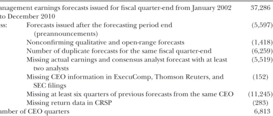
We obtain CEO information from the ExecuComp database. In addition, we follow Rogers and Van Buskirk [2009] and extract CEO information from the Thomson Financial Insider Trading database and the Securities and Exchange Commission’s (SEC) EDGAR database (we provide addi-tional details on this procedure in appendix A).8 We match our forecast data with the corresponding First Call reported earnings and analyst fore-casts, where we use the same split-adjusted basis to calculate forecasts and realized earnings per share. Our initial sample consists of 37,286 CEO-quarter observations (including forecasts that were “bundled” with earn-ings announcements). We next deleted forecasts issued after the forecast-ing period ends (Ajinkya, Bhojraj, and Sengupta [2005], Rogers [2008], Hilary and Hsu [2011]; 5,597 observations). Our sample includes point, range, and confirming qualitative forecasts (deleting nonconfirming qual-itative and open-ended forecasts leads to the further loss of 1,418 observa-tions). Following Roger and Stocken [2005], we removed duplicate fore-casts for the same fiscal quarter-end (6,259). We also delete observations for which earnings or consensus forecasts were missing (5,519),9for which
CEO information was missing (152), for which we have fewer than six quar-ters of forecasts issued by the same CEO (11,245), and for which data were missing in CRSP (283). Our final sample contains 6,813 CEO-quarters to es-timate model (1) and 59,105 CEO-analyst-quarters to eses-timate model (2). Table 1 summarizes the attrition in our sample.
6Our results do not change if we use at least five or seven quarters over the previous two
years to calculate forecast consistency and accuracy.
7Although our initial sampling period starts in 1994, when the management forecast
be-come available in the First Call database, our sample requirements are such that we do not get any observations before 1997. In addition, we would only gain 25 observations by adding observations from 1997 to 2001. We have deleted these 25 observations to increase data consis-tency. Our results are very similar if these observations are included (untabulated results). To further increase data consistency and mitigate the potential bias introduced via the different distribution of earlier forecasts, we focus on the last forecast made by a given manager before the end of the fiscal period (Hilary and Hsu [2011]).
8Our results hold when we use only the ExecuComp sample.
9Following Hilary and Hsu [2011], we require that there be at least two analysts who
is-sued forecasts in the previous 90 days but our results are not affected by this requirement (untabulated result).
T A B L E 1
Sample Selection Procedures
Management earnings forecasts issued for fiscal quarter-end from January 2002 to December 2010
37,286 Less: Forecasts issued after the forecasting period end
(preannouncements)
(5,597) Nonconfirming qualitative and open-range forecasts (1,418) Number of duplicate forecasts for the same fiscal quarter-end (6,259) Missing actual earnings and consensus analyst forecast with at least
two analysts
(5,519) Missing CEO information in ExecuComp, Thomson Reuters, and
SEC filings
(152) Missing at least six quarters of previous forecasts from the same CEO (11,245)
Missing return data in CRSP (283)
Number of CEO quarters 6,813
T A B L E 2
Summary Statistics
Variables N Mean SD 25% Median 75%
CONS 6,813 0.845 0.362 1.000 1.000 1.000 ACCU 6,813 0.486 0.500 0.000 0.000 1.000 ARET 6,813 0.002 0.084 −0.039 0.002 0.046 AFREV 59,105 −0.001 0.003 −0.001 0.000 0.001 NEWS Raw 6,813 −0.000 0.004 −0.001 0.000 0.002 NEWS FixAdj 6,813 −0.000 0.004 −0.001 0.001 0.002 NEWS Adj 6,162 0.001 0.004 0.000 0.001 0.003
CONSis the management forecast consistency andACCUis the management forecast accuracy (see appendix B for details).ARETis the three-day, size-adjusted stock return around the management forecast announcement.AFREVis an individual analyst’s forecast revision scaled by the stock price at the beginning of quartert.NEWS Rawis the difference between management forecast and consensus analyst forecast issued up to 90 days before the management forecast date, scaled by the stock price at the beginning of quartert.NEWS FixAdjis the difference between the management forecast (adjusted forMF FixBias, see appendix B) and the most recent consensus analyst forecast up to 90 days before the management forecast date, scaled by the stock price at the beginning of quartert.NEWS Adjis the difference between the management forecast (adjusted onMF Bias; see appendix A) and the most recent consensus analyst forecast up to 90 days before the management forecast date, scaled by the stock price at the beginning of quartert.NEWS Raw,NEWS FixAdj, andNEWS Adjare adjusted for “bundle” effect (Rogers and Van Buskirk [2013], in appendix A).
4. Empirical Results
4.1 DESCRIPTIVE STATISTICS
Table 2 provides descriptive statistics for the main variables used in our analysis. The mean value ofCONSis 0.85, suggesting a reasonably large de-gree of consistency in management forecasts compared to analyst forecasts. This result is consistent with the notion that managers have an information advantage over analysts when they forecast earnings for their own firms. In contrast, the mean value ofACCUis only 0.49, consistent with Hutton, Lee, and Shu [2012], who find that managers are not more accurate than analysts on average. The meanARETandAFREVare close to zero (0.002 and –0.001) and the standard deviations are comparatively high (0.084 and 0.003). Similarly,NEWS Raw,NEWS FixAdj, andNEWS Adjare on average
close to zero (–0.000, –0.000, and 0.001, respectively, with a standard devia-tion of 0.004 in all three cases). We lose 651 addidevia-tional observadevia-tions when we calculateNEWS Adjdue to the additional data requirement to estimate
MF Bias. Untabulated results indicate that only 20% of forecasts are issued with an upward bias (i.e.,MFE>0). Untabulated results also show that the mean absolute value of the difference between actual management forecast error (MFE) and predicted bias (MF Bias) is 25% smaller for highly consis-tent managers (CONS=1) than for low consistent ones (CONS=0). The average difference is statistically significant at less than 1% (one-sided test). This preliminary result suggests that it is easier to predict the bias when managers are more consistent.
The Pearson correlation matrix in table 3 indicates that the degree of cor-relation between ACCUandCONS is reasonably low (0.26). Similarly, the correlation of NEWS Raw,NEWS FixAdj, and NEWS Adj with ARET (0.29, 0.33, and 0.28, respectively) andAFREV(0.36, 0.53, and 0.43, respectively) is moderate. Finally, the three measures ofNEWSare positively correlated as expected (between 0.56 and 0.84). Panel B of table 3 provides the cor-relation between the three measures ofNEWSand ARETor AFREV, con-ditionally on the value of CONS. Results indicate that the correlation be-tween the news contained in the management forecasts and the reaction by users is approximately two to three times as large whenCONSequals one than whenCONSequals zero. The difference is statistically significant at less than 0.001 in all cases (one sided). These preliminary results are consistent with our main hypotheses that users of forecasts react more (per unit of “news”) when the consistency of the forecasts is greater. Panel C provides a similar analysis conditionally on the value ofACCU. We observe that the correlation between the news contained in the management forecasts and the reaction by users is greater when ACCUequals one than whenACCU
equals zero. However, the magnitude of the difference is smaller in panel C than in panel B in all six cases (at the 1% level in all six cases). In ad-dition, the difference in the correlation between ARETandNEWS FixAdj
(betweenACCU=1 andACCU=0) is insignificantly different from zero in panel C.
4.2 INVESTOR REACTION
Table 4 presents results from model (1). Column (1) tabulates the re-sults when we use NEWS FixAdj, while column (2) reports those when we
use NEWS Adj.The results indicate that the market reaction to
manage-ment forecasts is positively associated with managemanage-ment forecast consis-tency in both cases. The coefficients onCONS×NEWS FixAdjandCONS×
NEWS Adj are 4.151 and 4.367, respectively. They are both significant at
the 1% level (z-statistics equal 5.66 and 4.21, respectively). Untabulated analysis shows that our results continue to hold when we removeACCU× NEWSfrom the regression. The economic effect ofCONS ×NEWS FixAdj
T A B L E 3
Correlations Matrix
Panel A: Unconditional analysis
Variables CONS ACCU ARET AFREV NEWS Raw NEWS FixAdj
ACCU 0.26 ARET 0.01 −0.03 AFREV −0.01 −0.02 0.31 NEWS Raw 0.06 0.03 0.29 0.36 NEWS FixAdj 0.07 0.04 0.33 0.53 0.64 NEWS Adj 0.05 0.03 0.28 0.43 0.84 0.56
Panel B: Conditional analysis based onCONS
Correlations CONS=1 CONS=0 p-value for equality of correlations
Corr (ARET,NEWS Raw) 0.31 0.16 0.000∗∗∗
Corr (AFREV,NEWS Raw) 0.63 0.24 0.000∗∗∗
Corr (ARET,NEWS FixAdj) 0.31 0.17 0.000∗∗∗ Corr (AFREV,NEWS FixAdj) 0.62 0.22 0.000∗∗∗
Corr (ARET,NEWS Adj) 0.30 0.18 0.000∗∗∗
Corr (AFREV,NEWS Adj) 0.63 0.28 0.000∗∗∗
Panel C: Conditional analysis based onACCU
Correlations ACCU=1 ACCU=0 p-value for equality of correlations
Corr (ARET,NEWS Raw) 0.32 0.25 0.003∗∗∗
Corr (AFREV,NEWS Raw) 0.62 0.31 0.000∗∗∗
Corr (ARET,NEWS FixAdj) 0.31 0.28 0.197
Corr (AFREV,NEWS FixAdj) 0.60 0.36 0.000∗∗∗
Corr (ARET,NEWS Adj) 0.31 0.26 0.033∗∗
Corr (AFREV,NEWS Adj) 0.60 0.31 0.000∗∗∗
CONSis the management forecast consistency andACCUis the management forecast accuracy (see ap-pendix B for details).ARETis the three-day, size-adjusted stock return around the management forecast announcement.AFREVis an individual analyst forecast revision scaled by the stock price two days before the issuance of the management forecast.NEWS Rawis the difference between management forecast and consensus analyst forecast issued up to 90 days before the management forecast date, scaled by the stock price at the beginning of quartert.NEWS FixAdjis the difference between the management forecast (ad-justed forMF FixBias, see appendix B) and the most recent consensus analyst forecast up to 90 days before the management forecast date, scaled by the stock price at the beginning of quartert.NEWS Adjis the difference between the management forecast (adjusted onMF Bias, see appendix A) and the most recent consensus analyst forecast up to 90 days before the management forecast date, scaled by the stock price at the beginning of quartert.NEWS Raw,NEWS FixAdj, andNEWS Adjare adjusted for the “bundle” effect (Rogers and Van Buskirk [2013], in appendix A). The Pearson correlations in bold are significant at the 5% level or less. In panels B and C, the Pearson correlations that are significant at the 10%, 5%, and 1% levels are marked with∗,∗∗, and∗∗∗, respectively (two-tailed).
orCONS ×NEWS Adjis such that increasingCONS from 0 to 1 increases
the effect of NEWS FixAdj or NEWS Adj by approximately 50%.10 These results are consistent with H1a. In contrast, the coefficient on ACCU ×
NEWS FixAdj (ACCU × NEWS Adj, respectively) is insignificant and the
point estimate of the coefficient is only 30% (20%, respectively) of the esti-mate forCONS×NEWS FixAdj(CONS×NEWS Adj, respectively). However,
10We multiply the coefficients onCONS×NEWS FixAdjandCONS×NEWS Adj(4.151 and
T A B L E 4
The Effect of Consistency on the Market Reactions
(1) (2) (3) (4)
ARETi,t ARETi,t ARETi,t ARETi,t
NEWS FixAdj NEWS Adj NEWS Both NEWS Both
NEWSi,t 1.873∗∗∗ 2.789∗∗∗ 2.718∗∗∗ 8.393∗∗∗ (3.097) (3.838) (3.610) (2.717) CONSi,t 0.001 −0.004 0.002 0.002 (0.410) (−1.105) (0.726) (0.468) ACCUi,t −0.006∗∗ −0.007∗ −0.008∗∗∗ −0.008∗∗∗ (−2.148) (−1.975) (−2.966) (−2.944)
CONSi,t×NEWSi,t 4.151∗∗∗ 4.367∗∗∗ 4.393∗∗∗ 3.354∗∗∗
(5.658) (4.214) (5.411) (3.074)
ACCUi,t×NEWSi,t 1.437 0.849 1.421 0.399
(1.370) (0.801) (1.533) (0.413)
|NEWSi,t| ×NEWSi,t −5.566∗∗∗
(−6.169)
DAi,t-1×NEWSi,t 5.626
(0.461)
MTBi,t-1×NEWSi,t −0.121
(−0.450)
MFLOSSi,t×NEWSi,t 3.408∗∗∗
(3.025)
HORi,t×NEWSi,t −0.056
(−0.098)
RANGEi,t×NEWSi,t 1.799
(1.340)
MBESTREAKi,t×NEWSi,t 1.868
(0.935)
BADi,t×NEWSi,t −0.556
(−0.485)
AdjustedR2 0.093 0.087 0.105 0.121
Number of observations 6,813 6,162 5,957 5,957
This table reports the effects of management forecast consistency on the market reactions to the man-agement forecasts (ARET). All of the variables are defined in appendix B. The constant terms are included, but not tabulated. All of the continuous variables are winsorized at the 1st and 99th percentiles.Z-statistics (reported in parentheses) are corrected for heteroskedasticity and clustering of observations by CEO and quarter. Coefficients that are significant at the 10%, 5%, and 1% levels are marked with∗,∗∗, and∗∗∗, respectively (two-tailed).
ACCU×NEWS Adjbecomes significant with az-statistic of 3.07 whenCONS
and its interaction withNEWSare removed from the regression. The differ-ence betweenCONS×NEWS FixAdjandACCU×NEWS FixAdjorCONS×
NEWS AdjandACCU×NEWS Adjis statistically significant (the one-sided
p-value is less than 0.05 and 0.001, respectively).
A recent study by Hilary and Hsu [2013] shows that analysts also care more about consistency than accuracy, and thus issue forecasts that may be systematically biased to maintain good relations with managers. To address this issue, we compute a measure of news, NEWS Both, which is adjusted simultaneously for both the predictable bias in management forecasts
and in analyst forecasts.11Our approach to estimate the predicted analyst bias,AF Bias, is described in appendix A. We then reestimate model (1). Results presented in column (3) of table 4 do not change our conclusions.
CONS ×NEWS Bothremains significant andACCU×NEWS Bothremains
insignificant.12
Finally, we estimate an extended model that controls for various poten-tial confounding effects. Our vector of control variables contains those identified in previous studies that influence price formation (Rogers and Stocken [2005], in particular). Specifically, we control for growth oppor-tunities (MTB; Bamber and Cheon [1998], Rogers and Stocken [2005]), the predicted loss (MFLOSS; Hayn [1995], Rogers and Stocken [2005]), forecast range (RANGE; Baginski, Conrad, and Hassell [1993], Rogers and Stocken [2005]), consistency in meeting-or-beating consensus analyst fore-cast (MBESTREAK; Kross, Ro, and Suk [2011]), the amount of discretionary accruals (DA; Rogers and Stocken [2005]), forecast horizon (HOR; Kasznik [1999], Rogers and Stocken [2005]), the sign of management forecast news (BAD; Jennings [1987], Rogers, Skinner, and Van Buskirk [2009]), and the importance of the news (|NEWS|; Lipe, Bryant, and Widener [1998], Rogers and Stocken [2005]). All of these control variables are defined in greater detail in appendix B.
Again, results in column (4) of table 4 indicate that our conclusions are not affected and CONS × NEWS Bothremains significant.13 However, we
note that the average variation inflation factors (VIF) are approximately 13 in the last column of table 4 (with a maximum value over 64), suggest-ing the presence of strong multicollinearity in this specification. Thus, we focus on the specification reported in the first two columns as our base-line model. Our results hold if we examine several additional specifica-tions (untabulated results), for example, if we include the vector of con-trol variables (BAD, RANGE, HOR, MBESTREAK, |NEWS|, DA, MTB, and
MFLOSS) without the interactions. They also hold if we add firm size (SIZE; Baginski, Conrad, and Hassell [1993]), leverage (LEV; Collins and Kothari [1989]), analyst following (COVER; Lang and Lundholm [1996]), and earn-ings volatility (EARNVOL; Imhoff and Lobo [1992]) to the vector of con-trol variables and interact these variables withNEWS Both. Similarly, they hold if we include earnings announcement news (EANEWS) and its interac-tions with|EANEWS|,DA,MTB, andBAD EA(Rogers and Stocken [2005]).
11We also adjustNEWS Bothfor the “bundle” effect by following Rogers and Van Buskirk
[2013].
12We reach similar conclusions if we useNEWS FixBothinstead ofNEWS Both(untabulated
result).NEWS FixBothis similar toNEWS Bothbut we useMF FixBiasandAF FixBiasinstead of
MF BiasandAF Biasto adjustNEWS.AF FixBiasis calculated as the averaged value of analyst
forecast error (AFE) for a given CEO.
13Untabulated results indicate thatCONS×NEWS FixAdj,CONS×NEWS Adj, orCONS×
NEWS FixBothis also significant if we substitute them forCONS×NEWS Bothin this extended
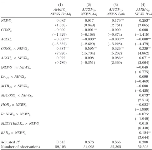
T A B L E 5
The Effect of Consistency on the Analyst Revisions
(1) (2) (3) (4)
AFREVi,j,t AFREVi,j,t AFREVi,j,t AFREVi,j,t
NEWS FixAdj NEWS Adj NEWS Both NEWS Both
NEWSi,t 0.085∗ 0.017 0.176∗∗∗ 0.253∗∗ (1.858) (0.849) (2.731) (3.065) CONSi,t −0.000 −0.001∗∗∗ −0.000 −0.000 (−1.329) (−6.168) (−0.874) (−1.415) ACCUi,t −0.000∗∗∗ −0.000∗∗ −0.000∗∗∗ −0.000∗∗∗ (−3.332) (−2.629) (−5.228) (−4.479)
CONSi,t×NEWSi,t 0.387∗∗∗ 0.595∗∗∗ 0.326∗∗∗ 0.339∗∗∗
(7.920) (15.784) (5.232) (4.862)
ACCUi,t×NEWSi,t 0.022 −0.008 0.086∗∗ 0.071∗∗
(0.789) (−0.351) (2.360) (2.064)
|NEWSi,t| ×NEWSi,t −0.048
(−0.775)
DAi,t-1×NEWSi,t −0.099
(−0.469)
MTBi,t-1×NEWSi,t −0.000
(−0.425)
MFLOSSi,t×NEWSi,t 0.073∗∗
(2.514)
HORi,t×NEWSi,t −0.023∗∗
(−1.989)
RANGEi,t×NEWSi,t −0.075∗
(−1.949)
MBESTREAKi,t×NEWSi,t 0.018
(0.440)
BADi,t×NEWSi,t 0.124∗∗∗
(3.644)
AdjustedR2 0.345 0.373 0.366 0.380
Number of observations 59,105 54,098 52,305 52,305
This table reports the effects of management forecast consistency on the analyst responses to the man-agement forecasts (AFREV). All of the variables are defined in appendix B. The constant terms are included, but not tabulated. All of the continuous variables are winsorized at the 1st and 99th percentiles.Z-statistics (reported in parentheses) are corrected for heteroskedasticity and clustering of observations by analyst, CEO, and quarter. Coefficients that are significant at the 10%, 5%, and 1% levels are marked with∗,∗∗, and ∗∗∗, respectively (two-tailed).
Although our conclusions are not affected, these different specifications further exacerbate the multicollinearity (the average VIF becomes 16 with a maximum of 95).
4.3 ANALYST REACTION
Table 5 presents results from model (2). Column (1) tabulates the results when we useNEWS FixAdj, whereas column (2) reports those when we use
NEWS Adj. The results indicate that the analyst forecast revision to
man-agement forecasts is positively associated with manman-agement forecast consis-tency in both cases. The coefficients onCONS ×NEWS FixAdjandCONS
×NEWS Adjare 0.387 and 0.595, respectively. They are significant at the
shows that our results continue to hold when we remove ACCU× NEWS
from the regression. These results are consistent with H1b. In contrast, the coefficients onACCU×NEWS FixAdjandACCU×NEWS Adjare insignif-icant (withz-statistics of 0.79 and –0.35), but become significant with az -statistic of 4.39 whenCONSand its interaction withNEWSare removed from the regression. The difference betweenCONS×NEWS FixAdjandACCU×
NEWS FixAdjor CONS ×NEWS Adjand ACCU× NEWS Adjis statistically
significant (the one-sidedp-value is less than 0.001 in both cases).
We then substituteNEWS BothforNEWS Adjand reestimate model (2). The results, presented in column (3) of table 5, do not change our con-clusions.CONS×NEWS Bothis significantly positive (thez-statistic is 4.86). The point estimate of the coefficient is approximately four times the value of the estimate of the coefficient forACCU×NEWS Both(the difference is significant with a one-sidedp-value lower than 0.001).14
Finally, we estimate the same extended model described in section 4.2. We report the results in column (4) of table 5. Again, our conclusions are not affected when we include a vector of control variables (BAD,RANGE,
HOR,MBESTREAK,|NEWS|,DA,MTB, andMFLOSS) and their interactions
with NEWS Both. CONS ×NEWS Both remains significant.15 However, the
average VIFs are approximately 11 in the last column of table 5 (with a maximum value of 67), again suggesting the presence of multicollinearity in this specification. Adding the vector of the aforementioned control vari-ables without the interactions, further controlling forSIZE, LEV,COVER,
andEARNVOL(and their interaction withNEWS Both), or including
earn-ings announcement news (EANEWS, and its interactions with |EANEWS|,
DA,MTB, andBAD EAas in Rogers and Stocken [2005]) does not affect our conclusions (untabulated results), but including the additional con-trol variables further exacerbates the multicollinearity (the average VIF be-comes 12 with a maximum of 83).
4.4 ADDITIONAL ROBUSTNESS CHECKS
We then perform different robustness checks (untabulated results). First, there may be a concern that the documented stock price reactions and analysts’ forecast revisions might be the result of earnings announcement news (Atiase, Rees, and Tse [2010]). To address this concern, we delete management forecasts made within –1 to+1 days of an earnings ment, using the Compustat quarterly file to identify the earnings announce-ment dates. This procedure results in a large number of observations be-ing removed from our sample and a much smaller sample size (1,485 vs. 6,162 in theARETspecification; 35,524 vs. 54,098 in theAFREVone). How-ever, this truncation does not affect our conclusions (untabulated result). 14We reach similar conclusions if we useNEWS FixBothinstead ofNEWS Both(untabulated
result).
15Untabulated results indicate thatCONS×NEWS FixAdj,CONS×NEWS Adj, orCONS×
CONS×NEWS Adjremains significant (withz-statistics of 3.95 and 12.39 for
ARETandAFREV, respectively) andACCU×NEWS Adjremains
insignifi-cant (withz-statistics of 0.88 and –0.28 forARETandAFREV, respectively). Second, our results continue to hold when we useNEWS Raw(instead of
NEWS FixAdjorNEWS Adj) to estimate models (1) and (2), as well as when
we use either the averaged value of MFEover the last two years (instead of over the CEO’s tenure) or the Kross, Ro, and Suk [2011] specification (instead of Rogers and Stocken [2005] specification) to debias NEWSin our baseline models.
Third, Rogers and Stocken [2005] find that the market predicts and fil-ters bias from management earnings forecasts. We implicitly rely on this finding when we use debiased versions of the forecasts. However, if investors and analysts only cared about accuracy, they would not adjust the fore-cast for the predicted bias and, therefore,ACCUshould be interacted with
NEWS Raw.To investigate this possibility, we reestimate models (1) and (2) substitutingACCU×NEWS RawforACCU×NEWS Adj, addingNEWS Raw,
and keeping CONS × NEWS Adj and NEWS Adj. CONS × NEWS Adj
re-mains significant (at the 1% level) and the difference between ACCU ×
NEWS RawandCONS×NEWS Adjis significant at the 5% level or better
(one sided).
Fourth, one could argue that we should measure consistency relative to a debiased forecast. This is not an issue if the bias is constant but it could be one if the bias is time varying. To investigate this question, we calculate the standard deviation of the adjusted management forecast errors (i.e., actual error, MFE, minus the estimated management bias, MF Bias) and calculateCONS Adjbased on the standard deviation of the adjusted man-agement forecast errors relative to the standard deviation of adjusted con-sensus analyst forecast errors (i.e., actual error,AFE, minus the estimated analyst bias,AF Bias). Untabulated results indicate that our conclusions are not affected.CONS Adj×NEWS Adjremains significant (with az-statistic of 4.75 in theARETspecification and 2.15 in theAFREVone).16
Fifth, we examine other alternative measures of management forecast consistency. For example, we defineCONS 50, measured as one ifSTDAFE
exceedsSTDMFEby more than the median value of the difference between
STDAFEandSTDMFE. That is, we construct a consistency measure that is
equal to one only half of the time. The mean value ofCONS 50 is 0.506 and the median value (by construction) is 0.500. Our conclusions are not affected. The z-statistics for CONS 50 × NEWS Adj are 3.12 in the ARET
specification and 4.74 in the AFREVone. Alternatively, we rank all of the CEOs by industry (four-digit SIC codes) in quartertbased on the standard deviation of forecast errors scaled by the stock price at the beginning of 16We also defineACCU Adjbased on the absolute value of the adjusted management
fore-cast errors relative to the absolute value of the adjusted analyst forefore-cast errors.ACCU Adj
×NEWS Adjremains insignificant in theAFREVspecification but becomes significant in the
the quarter. We then compute a consistency ranking score using the for-mula (Hong and Kubik [2003], Hilary and Hsu [2013]):CONS Rk =1 – (rank – 1)/(number of CEOs within the industry – 1). Similarly, we
esti-mateACCU Rkby ranking all of the CEOs within the same industry in each
quarter based on accuracy and calculate the mean of the ranking scores over the last two years.17 Our conclusions are not affected. CONS Rk ×
NEWS Adjremains significant in our baseline regressions (withz-statistics of 2.66 forARETand 2.51 forAFREV) andACCU Rk×NEWS Adjremains insignificant (withz-statistics of –0.33 forARETand –0.23 forAFREV).
Sixth, we delete observations that are both accurate and consistent (i.e., those for which bothCONSandACCUare equal to one). In this case, the correlation betweenCONS and ACCUbecomes –0.38. Again, our conclu-sions are not affected. CONS × NEWS Adj remains significant (with a z -statistic of 3.82 forARETand 4.61 forAFREV) andACCU×NEWS Adj re-mains insignificant or only weakly significant (with az-statistic of –0.40 for
ARETand 2.04 forAFREV).
5. Conditional User Reactions
In this last section, we examine whether users are aware of the systematic bias and whether this awareness depends on the consistency of the forecast. Further, we examine if the degree of sophistication of forecast users or the visibility of the bias influences their reactions.
5.1 TYPES OF NEWS AND PREDICTED BIAS
Our preliminary results in section 4.1 suggest that it is easier to predict management bias when forecasts are more consistent. Following Rogers and Stocken [2005], we posit that users filter bias more easily when fore-casts are more consistent. We estimate two models similar to that in Rogers and Stocken [2005] (i.e., their model (2)), but we partition the sample based on the median value ofSTDMFE. Specifically, we estimate:
ARETi,t =a0+a1NEWS Rawi,t+a2NEWS Rawi,t×M F Biasi,t
×GOODi,t+a3NEWS Rawi,t×M F Biasi,t×BADi,t
+akCONTROLSi,t+εi,t,
(3)
AFREVi,j,t =b0+b1NEWS Rawi,t+b2NEWS Rawi,t×M F Biasi,t
×GOODi,t+b3NEWS Rawi,t×M F Biasi,t×BADi,t
+bkCONTROLSi,t+εi,t.
(4) If investors and analysts do indeed filter bias more easily when man-agerial forecasts are more consistent, we expect the coefficient (in abso-lute value) associated withNEWS Raw×MF Bias×GOODandNEWS Raw
17This method of definingACCUis similar to that used in Hong and Kubik [2003],
ex-cept that we rank all CEOs within an industry based on quarterly forecast accuracy instead of ranking all analysts within a firm based on annual forecasts.
T A B L E 6
Test of Rogers and Stocken [2005] Conditional on the Consistency of Management Forecasts
ARETi,t AFREVi,j,t
(1) (2) (3) (4)
Low High Low High
STDMFE STDMFE STDMFE STDMFE
NEWS Rawi,t 3.330 0.508 0.592∗∗∗ 0.647∗∗∗
(3.433) (2.803) (4.454) (7.475)
NEWS Rawi,t×MF Biasi,t×GOODi,t −3.323∗ −1.442∗∗∗ −1.123∗∗ 0.250
(−1.809) (−4.556) (−2.451) (0.934)
NEWS Rawi,t×MF Biasi,t×BADi,t 3.089∗∗∗ 0.157∗∗∗ 0.673∗∗ 0.304∗∗∗
(2.850) (4.271) (2.055) (2.801)
NEWS Rawi,t× |NEWS Rawi,t| −0.000 −0.000∗∗∗ −0.047 −0.002
(−0.204) (−2.841) (−0.645) (−1.336)
NEWS Rawi,t×DAi,t-1 −3.810 0.289 −1.431∗ −0.001
(−0.116) (0.035) (−1.949) (−0.005)
NEWS Rawi,t×MTBi,t-1 −0.066 0.707∗∗∗ −0.000∗ −0.013
(−0.129) (2.613) (−1.662) (−1.259)
NEWS Rawi,t×MFLOSSi,t 0.000 0.610 0.441∗∗∗ 0.147∗∗∗
(0.000) (0.656) (2.597) (2.922)
NEWS Rawi,t×HORi,t −5.613∗∗∗ −0.791∗∗ −0.002 0.018
(−2.585) (−2.326) (−0.044) (1.011)
NEWS Rawi,t×RANGEi,t 1.567 −0.274 0.053 −0.112∗∗∗
(0.557) (−0.160) (0.552) (−2.335)
NEWS Rawi,t×MBESTREAKi,t 3.279 0.395 −0.090 −0.012
(0.844) (0.507) (−1.518) (−0.169)
AdjustedR2 0.091 0.089 0.398 0.431
Number of observations 3,094 3,098 27,664 26,384
This table reports the estimation results based on the model (2) in Rogers and Stocken [2005]. We par-tition the sample based on the median management forecast consistency (STDMFE). Columns (1) and (2) report the estimation results of the market reactions (ARET). Columns (3) and (4) report the estimation results of analyst revisions (AFREV). All of the variables are defined in appendix B. The constant terms are included, but not tabulated. All of the continuous variables are winsorized at the 1st and 99th per-centiles.Z-statistics (reported in parentheses) in columns (1) and (2) are corrected for heteroskedasticity and clustering of observations by CEO and quarter and those in columns (3) and (4) are by CEO, analyst, and quarter. Coefficients that are significant at the 10%, 5%, and 1% levels are marked with∗,∗∗, and∗∗∗, respectively (two-tailed).
× MF Bias × BAD to be larger in a sample of high consistency.18
Re-sults in table 6 are consistent with our conjecture and with Rogers and Stocken [2005]. Specifically, we find that the magnitude of coefficients on
NEWS Rawi,t×MF Biasi,t×GOODi,tandNEWS Rawi,t×MF Biasi,t×BADi,t are larger (in absolute value) in the sample of consistent forecasts than in the sample of inconsistent forecasts. The difference in the estimates for these coefficients across the two samples is statistically significant (with one-sidedp-values approximately equal to 0.008 and 0.058 in theARET specifi-cation and to 0.085 and 0.003 in theAFREVspecification).19
18GOOD(BAD) is an indicator variable that equals one ifNEWSis positive (negative), zero
otherwise. The results are not affected if we useMF FixBiasinstead ofMF Biasin the test.
19Our results are not affected if we follow Rogers and Stocken [2005] to further include
5.2 USER SOPHISTICATION
Our basic intuition is that investors and analysts should prefer biased but consistent forecasts rather than unbiased forecasts that are relatively more accurate but inconsistent if they can detect systematic bias. There-fore, the effect of consistency on the usefulness of management forecasts should be affected by the ability (sophistication) of investors and analysts to understand the systematic bias introduced by managers. Prior research sug-gests that institutional investors are more sophisticated than retail investors (Boehmer and Kelley [2009], Campbell, Ramadorai, and Schwartz [2009], Puckett and Yan [2011]), and that analysts with greater experience forecast earnings more accurately (Mikhail, Walther, and Willis [1997], Clement [1999], Jacob, Lys, and Neale [1999]) and are less overoptimistic regarding accruals (Drake and Myers [2011]). Our hypotheses rely on the assumption that users behave in a Bayesian fashion and understand the importance of consistency in forecasting, an ability that we would expect to be more com-mon acom-mong sophisticated, experienced users.20To test this conjecture, we
estimate model (1) conditional on the percentage of institutional investors (INTO) in the shareholding of the firm. Similarly, we estimate model (2) conditional on the amount of experience (EXP) analysts have.
Our results are reported in table 7. They indicate that sophisticated in-vestors focus on consistent forecasts. In column (1),CONS×NEWS Adjis significantly positive with az-statistic of 3.94 in the sample of high institu-tional ownership, whileACCU×NEWS Adjis insignificant (with az-statistic of –0.71). In contrast, column (2) shows thatCONS×NEWS Adjis insignifi-cant in the sample of low institutional ownership (with az-statistic of –0.51), whileACCU×NEWS Adjis significantly positive (with az-statistic of 10.58). The differences between the estimates forCONS ×NEWS Adj andACCU
×NEWS Adjacross the two samples are significantly different withp-values lower than 0.001 (one sided) in both cases.
Similarly, results in table 7 indicate that experienced analysts focus on consistent forecasts. In column (3),CONS×NEWS Adjis significantly pos-itive in the sample of experienced analysts (with az-statistic of 6.82), but insignificant in the sample of inexperienced analysts (with a z-statistic of 1.17), tabulated in column (4). The difference between the estimates across the two samples is significant with a p-value less than 0.001 (one sided). Column (4) shows that the point estimate of the coefficient ofACCU × NEWS Adjis twice as large in the sample of inexperienced analysts as in the
BAD EAin model (3) (untabulated results), but this further exacerbates the multicollinearity
(the average VIF becomes 30 with a maximum of 140).
20If investors are unable to debias forecasts, managers may try to manipulate investors’
expectations. However, if investors are able to debias forecasts, manipulation is futile. In this case, as discussed in section 2, we expect the bias to exist because users expect it to occur. The prior literature (e.g., Rogers and Stocken [2005], Hilary and Hsu [2013]) suggests that the market reaction to the bias is efficient on average but that users in certain subsamples may be functionally fixated.
T A B L E 7
Partition Tests Conditional on Investor Sophistication and Analyst Experience
ARETi,t AFREVi,j,t
(1) (2) (3) (4)
High Low High Low
INTO INTO EXP EXP
NEWS Adji,t 3.279∗∗∗ 0.003 0.133∗∗ 0.513
(3.284) (0.048) (2.273) (3.637)
CONSi,t −0.002 0.001 −0.001∗∗∗ −0.000
(−0.407) (0.192) (−4.072) (−1.248)
ACCUi,t −0.006 −0.013∗∗∗ −0.000∗∗∗ −0.001∗∗∗
(−1.639) (−3.568) (−4.430) (−3.271)
CONSi,t×NEWS Adji,t 5.043∗∗∗ −0.212 0.397∗∗∗ 0.049
(3.937) (−0.506) (6.820) (1.186)
ACCUi,t×NEWS Adji,t −0.812 8.822∗∗∗ 0.144∗∗∗ 0.290∗∗
(−0.713) (10.584) (3.046) (2.462)
AdjustedR2 0.093 0.061 0.380 0.260
Number of observations 3,017 2,872 25,202 25,466
This table reports the effects of management forecast consistency on the market reactions and analysts’ forecast revisions to the management forecasts. We partition the sample by the median institutional own-ership (INTO) and report the estimation results of market reactions (ARET) in columns (1) and (2). We partition the sample by the median analyst experience (EXP) and report the estimation results of analyst revisions (AFREV) in columns (3) and (4). We adjustNEWSforMF Bias. All of the variables are defined in appendix B. The constant terms are included, but not tabulated. All of the continuous variables are win-sorized at the 1st and 99th percentiles.Z-statistics (reported in parentheses) in columns (1) and (2) are corrected for heteroskedasticity and clustering of observations by CEO and quarter and those in columns (3) and (4) are by CEO, analyst, and quarter. Coefficients that are significant at the 10%, 5%, and 1% levels are marked with∗,∗∗, and∗∗∗, respectively (two-tailed).
sample of experienced analysts. However, the coefficients are statistically significant in both samples and the difference across the two samples is not significant.
5.3 SIZE OF THE BIAS
Finally, we partition our sample into two subsamples based on the size of the bias using the median of AbsMF Bias(i.e., absolute value ofMF Bias), although our results are not affected if we use the absolute value of
MF FixBiasinstead (untabulated result). We then reestimate the effect of
consistency on forecast informativeness separately for each subsample. This allows us to better distinguish between consistency and accuracy by investi-gating whether consistency is more relevant to investors when stated accu-racy is low. We expect this to be true because users should value consistency rather than accuracy in the presence of large systematic deviations from realized earnings. In other words, we expect forecast users to detect and correct for biases that are larger (in absolute value) and hence more visible. Results reported in table 8 are consistent with this intuition. They indi-cate that investors focus on the consistent forecasts when the size of the systematic bias is large. In column (1),CONS ×NEWS Adjis significantly positive with a z-statistic of 4.93 in the sample of high AbsMF Bias, while
ACCU ×NEWS Adjis insignificant (with a z-statistic of 0.84). In contrast, column (2) shows thatCONS×NEWS Adjis insignificant in the sample of
T A B L E 8
Partition Tests Conditional on the Size of Bias
ARETi,t AFREVi,j,t
(1) (2) (3) (4)
High Low High Low
AbsMF Bias AbsMF Bias AbsMF Bias AbsMF Bias
NEWS Adji,t 1.595∗∗ 0.687 0.162∗∗ 0.354∗∗∗
(2.780) (0.415) (2.164) (7.725)
CONSi,t −0.006 0.007 −0.001∗∗∗ 0.000∗∗
(−1.484) (1.304) (−2.904) (2.013)
ACCUi,t −0.006 −0.017∗∗∗ −0.001∗∗∗ −0.000∗∗
(−1.329) (−4.964) (−3.835) (−2.417)
CONSi,t×NEWS Adji,t 3.939∗∗∗ −0.876 0.389∗∗∗ −0.008
(4.925) (−0.526) (5.625) (−0.701)
ACCUi,t×NEWS Adji,t 0.897 8.244∗∗∗ 0.198∗∗ 0.179∗∗∗
(0.835) (7.291) (2.340) (2.973)
AdjustedR2 0.111 0.074 0.444 0.263
Number of observations 3,151 3,011 27,253 26,829
This table reports the effects of management forecast consistency on the market reactions and analysts’ forecast revisions to the management forecasts. We partition the samples based on the size of manage-ment forecast bias (AbsMF Bias). Columns (1) and (2) report the estimation results of the market reactions (ARET) and columns (3) and (4) report the estimation results of analyst revisions (AFREV). We adjustNEWS
forMF Bias. All of the variables are defined in appendix B. The constant terms are included, but not tabu-lated. All of the continuous variables are winsorized at the 1st and 99th percentiles.Z-statistics (reported in parentheses) in columns (1) and (2) are corrected for heteroskedasticity and clustering of observations by CEO and quarter and those in columns (3) and (4) are by CEO, analyst, and quarter. Coefficients that are significant at the 10%, 5%, and 1% levels are marked with∗,∗∗, and∗∗∗, respectively (two-tailed).
lowAbsMF Bias (with az-statistic of –0.53), whereasACCU ×NEWS Adjis
significantly positive (with az-statistic of 7.29). The differences between the estimates forCONS×NEWS AdjandACCU×NEWS Adjacross the two sam-ples are significantly different, withp-values lower than 0.003 (one sided) in both cases.
Similarly, our results in table 8 indicate that analysts focus on consistency of forecasts when the size of the systematic bias is large. In column (3),
CONS×NEWS Adjis significantly positive in the sample of highAbsMF Bias
(with az-statistic of 5.63) but insignificant in the sample of smallAbsMF Bias
(with a z-statistic of –0.70) tabulated in column (4). The differences be-tween the estimates across the two samples are significant with ap-value less than 0.001 (one sided). In contrast, our results indicate that the size of the bias does not affect the importance of forecast accuracy for analysts.
6. Conclusions
We examine the role of management forecast consistency in the capi-tal markets. We show that managers with higher forecast consistency have a greater ability to move prices and influence analyst revisions. The ef-fect is both economically and statistically significant. Consistent with pre-vious work, we find some support for the notion that accuracy influences market reactions and analyst revisions, but its effects are generally weaker
than those of consistency. Indeed the effect of accuracy often disappears once we control for consistency. In contrast, the effect of consistency is ro-bust to a host of specification checks. For example, the effect persists when we adjust for systematic biases in management and analyst forecasts (Rogers and Stocken [2005]), identify non-ExecuComp executives (Rogers and Van Buskirk [2009]), and use “bundled” forecasts (Rogers and Van Buskirk [2013]). The effect also persists after controlling for a host of potential confounds (e.g., Jennings [1987], Baginski, Conrad, and Hassell [1993], Kross, Ro, and Suk [2011]).
We also find that it is easier to predict the bias when managers are more consistent and that investors and analysts filter systematic bias in manage-ment forecasts more easily when the forecasts are more consistent. We next consider if the degree of user sophistication and of bias visibility affects the understanding of the forecast properties. Our empirical results suggest that this is indeed the case. Specifically, institutional investors and experienced analysts react more to consistent forecasts than retail investors and inexpe-rienced analysts. Finally, the effect of consistency on investor reactions and analyst revisions is more significant when bias is more visible.
APPENDIX A
Additional Details on Methodology and Sampling Procedure
A.1THE ESTIMATION OF MANAGEMENT FORECAST BIAS(MF BIAS)
We follow Rogers and Stocken [2005] to calculate management forecast bias (MF Bias) as the fitted value of management forecast error from the following regression estimated with quarterly data for management fore-casts (firm and time subscripts omitted):
M F E =a0+a1Di f f i c ult y+a2Li tig ati on+a3Li tig ati on×Di f f i c ult y
+a4I ns i de Tr ade+a5I ns i de Tr ade×Di f f i c ult y+a6Di s tr e s s
+a7Di s tr e s s×Di f f i c ult y+a8Conc e n+a9Conc e n×Di f f i c ult y
+a10Bad N e w s+a11N e w s Raw×Good N e w s
+a12N e w s Raw×Bad N e w s+a13H or i zon+a14CAR−120,−1
+a15Si ze+a16M/BRank+a17DAc cr uals
+year and industry fixed effects+ε.
(A.1)
MFEis the management forecast error, defined as the difference between management forecast and actual earnings, scaled by stock price.Difficulty
is forecasting difficulty, combining the effects of lack of analyst consen-sus (STD AF), the difficulty analysts experienced when predicting earnings (STD AFE), lagged loss (Lagged Loss), predicted loss (MFLOSS), volatility in a firm’s stock price (STD RET), bid-ask spread (Spread), and manager-revealed uncertainty (RANGE) by using principal axis factoring (PAF). Lit-igation is the probability of litigation.Inside Trade is the ranked value of the net insider purchases over the 10-trading-day window beginning on the day of the forecast.Distressis financial distress, defined asZ-score.Concenis
industry concentration, measured by the Herfindahl index, which equals the sum of the squares of the market shares of the firms within a four-digit SIC industry.News Rawis the management forecast news, measured as the difference between management forecast and consensus analyst forecast, scaled by the stock price.Bad Newsis an indicator variable that equals one ifNews Rawis negative, and zero otherwise.Good Newsis an indicator vari-able that equals one ifNEWS Rawis equal to or greater than zero, and zero otherwise. Horizonis forecast horizon, measured as the number of calen-dar days between the forecast release date and the firm’s fiscal year-end.
CAR–120,–1is the cumulative daily return less the size-decile-matched CRSP
value-weighted index over the period 120 days before to one day before the forecast date.Sizeis firm size, measured as the natural log of the firm’s mar-ket capitalization one day prior to the forecast.M/B Rankis the decile rank of the market-to-book ratio, which is the market value of equity divided by the book value of equity at the end of the prior quarter.DAccrualsis discre-tionary accruals estimated using the cross-sectional modified Jones model (Brown and Pinello [2007]) scaled by the stock price.
A.2THE ESTIMATION OF“BUNDLED FORECAST EFFECTS”
Rogers and Van Buskirk [2013] suggest that evaluating management forecast news based on preforecast (and, therefore, preearnings) estimates is likely to yield a measure of forecast news that is both downwardly bi-ased and spuriously correlated with the contemporaneous earnings sur-prise. Therefore, we consider earnings announcement effect on bundled forecast news by estimating the following two-stage regressions (Rogers and Van Buskirk [2013]):
First stage regression:
Prob(Bundle d=1)=a0+a1ConferenceCall+a2MFIssued
+a3LastBundled+a4GoodEANews
+a5BadEANews+a6AbsEANews+a7Loss
+a8STD AF+a9Ret+a10SIZE+a11COVER
+a12FreqAFLowball+ year and industry
fixed effects+ε.
(A.2)
Bundled is an indicator variable that equals one if there is a
manage-ment forecast issued in the three-day window (–1, 1) around an earn-ings announcement date.ConferenceCallequals one for earnings announce-ments issued with a contemporaneous conference call, and zero otherwise. We collect conference call data from LexisNexis, Bloomberg, and Capi-talIQ. MFIssued equals one for earnings announcements for which man-agement had previously issued an earnings forecast, zero otherwise. Last-Bundledequals one if the firm issued a forecast at the prior quarter’s earn-ings announcement date, and zero otherwise.GoodEANewsequals one for earnings surprises (actual earnings minus analyst estimates, scaled by stock price) greater than 0.0001, and zero otherwise.BadEANewsequals one for