Weighted graph algorithms with Python

Weighted Graph Algorithms with Python

Andrzej Kapanowski

Marian Smoluchowski Institute of Physics, Jagiellonian University, Kraków, Poland [email protected]

Łukasz Gałuszka

Marian Smoluchowski Institute of Physics, Jagiellonian University, Kraków, Poland [email protected]

Abstract

Python implementation of selected weighted graph data structures and algorithms is presented. The minimal graph interface is defined together with several classes implementing this interface. Graph nodes can be any hashable Python objects. Directed edges are instances of the Edge class. Graphs are instances of the Graph class. It is based on the adjacency-list representation, but with fast lookup of nodes and neighbors (dict-of-dict structure). Other implementations of this class are also included, for instance, the adjacency matrix representation (list-of-list structure). Multigraphs are instances of the MultiGraph class.

In this work, many algorithms are implemented using a unified approach. There are separate classes and modules devoted to different algorithms. Three algorithms for finding a minimum spanning tree are implemented: the Boruvka's algorithm, the Prim's algorithm (three implementations), and the Kruskal's algorithm. Three algorithms for solving the single-source shortest path problem are implemented: the dag shortest path algorithm, the Bellman-Ford algorithm, and the Dijkstra's algorithm (two implementations). Two algorithms for solving all-pairs shortest path problem are implemented: the Floyd-Warshall algorithm and the Johnson's algorithm.

All algorithms were tested by means of the unittest module, the Python unit testing framework. Additional computer experiments were done in order to compare real and theoretical computational complexity. The source code is available from the public GitHub graphs-dict repository.

Keywords: graph theory, weighted graphs, graph algorithms.

1. Introduction

Algorithms are at the heart of computer science. They are expressed as a finite sequence of operations with clearly defined input and output. Algorithms can be expressed by natural languages, pseudocode, flowcharts or programming languages. Pseudocode is often used in textbooks and scientific publications because it is compact and augmented with natural language description. However, in depth understanding of algorithms is almost impossible without computer experiments, where algorithms are implemented by means of a programming language.

Our aim is to show that the Python programming language (Lutz, 2007) can be used to implement algorithms with simplicity and elegance. On the other hand, the code is almost as readable as pseudocode because the Python syntax is very clear. That is why Python has become one of the most popular teaching languages in colleges and universities (Shein, 2015), and it is used in scientific research (Perkel, 2015). Python implementation of some algorithms from computational group theory was shown in (Kapanowski, 2014). In this paper we are interested in graph theory and weighted graph algorithms. Other graph algorithms will be discussed elsewhere. The source code is available from the public GitHub graphs-dict repository (Kapanowski, 2015). We strongly support a movement toward open source scientific software (Hayden, 2015).

Graphs can be used to model many types of relations and processes in physical, biological, social, and information systems (Wikipedia, 2015f). Many practical problems can be represented by graphs and this can be the first step to finding the solution of the problem. Sometimes the solution can be known for a long time, because graph theory was born in 1736. In this year Leonard Euler solved the famous Seven Bridges of Königsberg (Królewiec in Polish) problem.

We examined several Python graph packages from The Python Package Index (PyPI, 2015) in order to checked different approaches. Some graph libraries written in other programming languages were also checked briefly (BGL, 2015), (Mehlhorn et al., 1999), (GTL, 2015).

• Package NetworkX 1.9 by Hagberg, Schult, and Swart (Hagberg et al., 2014). This is a library for the creation, manipulation, and study of the structure, dynamics, and functions of complex networks. Basic classes are Graph, DiGraph, MultiGraph, and MultiDiGraph. All graph classes allow any hashable object as a node. Arbitrary edge attributes can be associated with an edge inside a graph. However, stand-alone edges are 2-tuples or 3-tuples. The dictionary of dictionaries data structure is used to store graphs. Algorithms are usually functions grouped inside modules. Drawing graphs is possible with Matplotlib, pygraphviz, or Pydot.

• Package python-igraph 0.7.0 (igraph, 2015). igraph is the network analysis package with versions for R, Python, and C/C++. Basic clases are Vertex, VertexSeq, Edge, EdgeSeq, GraphBase, Graph, and other. Vertices and edges have continuous IDs and that is why deleting vertices or edges can be uncomfortable. Setting and retrieving attributes for vertices and edges is possible by means of special objects vs and es (sequences), respectively. igraph implements several layout algorithms and uses the Cairo library to draw graphs.

• Package graph-tool 2.2.43 by Peixoto (graph-tool, 2015). It is an efficient Python module for manipulation and statistical analysis of graphs. The core data structures are implemented in C++, making use of template metaprogramming, based on the Boost Graph Library (BGL, 2015). many algorithms are implemented in parallel using OpenMP.

• Package python-graph 1.8.2 by Matiello (Matiello, 2015). It is a library for working with graphs in Python. Edges are standard Python tuples, weights or labels are kept

separately. There are different classes for directed graphs, undirected graphs, and hypergraphs. Algorithms are functions grouped in modules.

• Package graph 0.4 by Robert Dick and Kosta Gaitanis (Dick et al., 2005). Directed and undirected graph data structures and algorithms are provided. Basic clases are Vertex, RawEdge, DirEdge, UndirEdge, Graph, Tree, and other. This is a relatively small project.

None of the available implementations satisfy our needs. We would like to get a pure Python implemenation of graph algorithms without dependency on third-party modules. A source code should be readable, because we would like to use it in education instead of pseudocode. We would like to present Python best practices. On the other hand, the real complexity of the algorithms should be consistent with the underlying theory. A user should run the code and solve medium-sized problems. We would like to use consistent graph interface. Some packages use 2-tuple and 3-tuple for edges, other packages use several edge classes; we prefer single Edge class. For graphs, we prefer two classes (Graph, Multigraph), because undirected graphs are internally smilar to directed graphs (an undirected edge is stored as two directed edges). Iterators through nodes and edges are prefered over returning full lists. Usually high computational efficiency leads to the unreadable code. On the other hand, C/C++ syntax or Java syntax are not very close to the pseudocode used for teaching. That is why we develop and advocate our approach. We note that presented Python implementations may be not as fast as C/C++ or Java counterparts but they scale with the input size according to the theory. The presented algorithms are well known and that is why we used references to many Wikipedia pages.

The paper is organized as follows. In Section 2 basic definitions from graph theory are given. In Section 3 the package installation is described. In Section 4 the graph interface is presented. In Sections 5, 6, and 7 the following algorithms are shown: for finding a minimum spanning tree, for solving the single-source shortest path problem, for solving all-pair shortest path problem. Conclusions are contained in Section 8.

2. Definitions

Definitions of graphs vary and that is why we will present our choice which is very common (Cormen et al., 2009). We will not consider multigraphs with loops and multiple edges. 2.1. Graphs

A (simple) graph is an ordered pair G = (V, E), where V is a finite set of nodes (vertices, points) and E is a finite set of edges (lines, arcs, links). An edge is an ordered pair of different nodes from V, (s, t), where s is the source node and t is the target node. This is a directed edge and in that case G is called a directed graph.

An edge can be defined as a 2-element subset of V, {s, t} = {t, s}, and then it is called an undirected edge. The nodes s and t are called the ends of the edge (endpoints) and they are adjacent to one another. The edge connects or joins the two endpoints. A graph with undirected edges is called an undirected graph. In our approach, an undirected edge

corresponds to the set of two directed edges {(s, t), (t, s)} and the representative is usually (s, t) with s < t.

The order of a graph G = (V, E) is the number of nodes |V|. The degree of a node in an undirected graph is the number of edges that connect to it. A graph G' = (V', E') is a subgraph of a graph G = (V, E) if V' is a subset of V and E' is a subset of E.

2.2. Graphs with weights

A graph structure can be extended by assigning a number (weight) w(s, t) to each edge (s, t) of the graph. Weights can represent lengths, costs or capacities. In that case a graph is called a weighted graph.

2.3. Paths and cycles

A path P from s to t in a graph G = (V, E) is a sequence of nodes from V, (v_0, v_1, ..., v_n), where v_0 = s, v_n = t, and (v_{i-1}, v_{i}) (I = 1, ..., n) are edges from E. The length of the path P is n. A simple path is a path with distinct nodes. The weight (cost or length) of the path in a weighted graph is the sum of the weights of the corresponding edges.

A cycle is a path C starting and ending at the same node, v_0 = v_n. A simple cycle is a cycle with no repetitions of nodes allowed, other than the repetition of the starting and ending node. A dag is a directed acyclic graph.

A directed path (cycle) is a path (cycle) where the corresponding edges are directed. In our implementation, a path is a list of nodes. A graph is connected if for every pair of nodes s and t, there is a path from s to t.

2.4. Trees

A (free) tree is a connected undirected graph T with no cycles. A forest is a disjoint union of trees. A spanning tree of a connected, undirected graph G is a tree T that includes all nodes of G and is a subgraph of G (Wikipedia, 2015l). Spanning trees are important because they construct a sparse subgraph that tells a lot about the original graph. Also some hard problems can be solved approximately by using spanning trees (e.g. traveling salesman problem). A rooted tree is a tree T where one node is designated the root. In that case, the edges can be oriented towards or away from the root. In our implementation, a rooted tree is kept as a dictionary, where keys are nodes and values are parent nodes. The parent node of the root is None. A forest of rooted trees can be kept in a dictionary with many roots.

A shortest-path tree rooted at node s is a spanning tree T of G, such that the path distance from root s to any other node t in T is the shortest path distance from s to t in G.

3. Installing the package

The graphs-dict repository contains the graphtheory package which depends on the Python Standard Library only. No additional Python modules (Numpy, Scipy) are required. The ZIP file with the graphtheory package one can download from the GitHub repository

(Kapanowski, 2015). On Linux and other Unix-like systems with git installed, the whole project can be cloned into the home directory

$ git clone https://github.com/ufkapano/graphs-dict.git $ cd graphs-dict

$ ls

doc graphtheory LICENCE README.md

The graphs-dict directory should be added to the PYTHONPATH environment variable, because it contains the graphtheory package. A user is encouraged to read the source code of the modules and the test files (test_*.py), because they provide many examples of use. Modules can be also customized to user's needs.

4. Interface for graphs

According to the definitions from Section 2, graphs are composed of nodes and edges. In our implementation nodes can be any hashable object that can be sorted. Usually they are integer or string.

Edges are instances of the Edge class (edges module) and they are directed, hashable, and comparable. Any edge edge1 has the starting node (edge1.source), the ending node (edge1.target), and the weight (edge1.weight). The default weight is one. The edge with the opposite direction to edge1 is equal to ~edge1. This is very useful for combinatorial maps used to represent planar graphs (Wikipedia, 2015c).

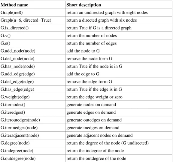
Simple graphs (directed and undirected) are instances of the Graph class. Three different implementations of the Graph class are available from different modules: graphs module, dictgraphs module, and matrixgraphs module (list-of-list structure). Multigraphs (directed and undirected) are instances of the MultiGraph class (multigraphs module) and they will not be discussed here. Many algorithms can work with simple graphs and multigraphs, because their interface is almost identical. Let us show some properties of graphs that are listed in Table 3.1. There are methods to report some numbers (nodes, edges, degrees). There are iterators over nodes and edges. There are also some logical functions.

>>> from graphtheory.structures.edges import Edge >>> from graphtheory.structures.graphs import Graph >>> G = Graph(n=3, directed=False)

# n is for compatibility with different implementations. >>> G.add_edge(Edge(source=0, target=1, weight=5))

>>> G.add_edge(Edge(source=0, target=2, weight=7)) # Nodes are automatically added with edges.

>>> G.v(), G.e(), G.is_directed()

(3, 2, False) # numbers of nodes and edges >>> list(G.iternodes())

[0, 2, 1] # random order of nodes

>>> sorted((G.degree(node) for node in G.iternodes()), reverse=True) [2, 1, 1] # the degree sequence

>>> list(node for node in G.iternodes() if G.degree(node) == 1) [2, 1] # leafs

>>> sum(edge.weight for edge in G.iteredges())

Method name Short description

Graph(n=8) return an undirected graph with eight nodes

Graph(n=6, directed=True) return a directed graph with six nodes

G.is_directed() return True if G is a directed graph

G.v() return the number of nodes

G.e() return the number of edges

G.add_node(node) add the node to G

G.del_node(node) remove the node form G

G.has_node(node) return True if the node is in G

G.add_edge(edge) add the edge to G

G.del_edge(edge) remove the edge form G

G.has_edge(edge) return True if the edge is in G

G.weight(edge) return the edge weight or zero

G.iternodes() generate nodes on demand

G.iteredges() generate edges on demand

G.iteroutedges(node) generate outedges on demand

G.iterinedges(node) generate inedges on demand

G.iteradjacent(node) generate adjacent nodes on demand

G.degree(node) return the degree of the node (G undirected)

G.indegree(node) return the indegree of the node

G.outdegree(node) return the outdegree of the node

Table 3.1. Interface for graphs; G is a graph, node is usually integer or string, edge is an instance of the Edge class.

Note that in the case of undirected graphs, edge and ~edge are two representatives of the same undirected edge. The method iteredges returns a representative with the ordering edge.source < edge.target.

The instruction Graph(n=8) has the parameter n (the number of nodes) which should be specified in the case of the adjacency matrix representation (matrixgraphs module). The parameter n is ignored if dict-of-dict structure is used (graphs module or dictgraphs module).

Graph algorithms are implemented using a unified approach. There is a separate class for every algorithm. Different implementations of the same algorithm are grouped in one module. In the __init__ method, main variables and data structures are initialized. The name space of a class instance is used to access the variables and that is why interfaces of the auxiliary methods can be very short.

5. Minimum spanning tree

Let us assume that G = (V, E) is a connected, undirected, weighted graph, and T is a spanning tree of G. We can assign a weight to the spanning tree T by computing the sum of the weights of the edges in T. A minimum spanning tree (MST) is a spanning tree with the weight less than or equal to the weight of every other spanning tree. In general, MST is not unique. There is only one MST if each edge has a distinct weight (Wikipedia, 2015i).

Minimum spanning trees have many practical applications: the design of networks, taxonomy, cluster analysis, and others (Wikipedia, 2015i). We would like to present three classical greedy algorithms for finding MST that run in polynomial time. The fact that a greedy strategy produces an optimal solution is not trivial. The theory of matroids provide an explanation (Cormen et al., 2009).

5.1. Boruvka's algorithm

The Boruvka's algorithm works for an undirected connected graph whose edges have distinct weights what implies the unique MST (Wikipedia, 2015i). In the beginning, the cheapest edge from each node to another in the graph is found, without regard to already added edges. Then joining these groupings continues in this way until MST is completed (Wikipedia, 2015b). Components of MST are tracked using a disjoint-set data structure. The algorithm runs in O(E log V) time.

Our implementation of the Boruvka's algorithm works also for disconnected graphs. In that case a forest of minimum spanning trees is created. What is more, repeated edge weights are allowed because our edge comparison use also nodes, when weights are equal (Wikipedia, 2015b).

>>> from graphtheory.spanningtrees.boruvka import BoruvkaMST >>> G = Graph(n=10, directed=False) # an exemplary graph # Add nodes and edges here.

>>> algorithm = BoruvkaMST(G)

>>> algorithm.run() # calculations

>>> algorithm.mst.show() # MST as an undirected graph

We note that the Boruvka's algorithm is well suited for parallel computation (Bader, Cong, 2006). However, our implementation is a serial one.

5.2. Prim's algorithm

The Prim's algorithm has the property that the edges in a growing spanning tree T always form a single tree. The weights from G can be negative (Wikipedia, 2015j). We begin with some node s from G and s is added to the empty T. Then, in each iteration, we choose a minimum-weight edge (s, t), joining s inside T to t outside T. Then the minimum-weight edge is added to T. This process is repeated until MST is formed.

The performance of Prim's algorithm depends on how the priority queue is implemented. In the case of the first implementation a binary heap is used and it takes O(E log V) time. >>> from graphtheory.spanningtrees.prim import PrimMST

>>> G = Graph(n=10, directed=False) # an exemplary graph # Add nodes and edges here.

>>> algorithm = PrimMST(G)

>>> algorithm.run() # calculations >>> algorithm.parent # MST as a dict

>>> mst = algorithm.to_tree() # MST as an undirected graph

The second implementation is better for dense graphs (|E| of order |V|2), where the adjacency-matrix representation of graphs is often used. For-loop is executed |V| times, finding the minimum takes O(V). Therefore, the total time is O(V2).

>>> from graphtheory.spanningtrees.prim import PrimMatrixMST >>> from factory import GraphFactory

>>> gf = GraphFactory(Graph)

>>> G = gf.make_complete(n=10, directed=False) # a weighted graph >>> algorithm = PrimMatrixMST(G)

>>> algorithm.run() # calculations >>> algorithm.parent # MST as a dict

>>> mst = algorithm.to_tree() # MST as an undirected graph

5.3. Kruskal's algorithm

The Kruskal's algorithm builds the MST in forest (Kruskal, 1956), (Wikipedia, 2015h). In the beginning, each node is in its own tree in its own forest. Then all edges are scanned in increasing weight order. If an edge connects two different trees, then the edge is added to the MST and the trees are merged. If an edge connects two nodes in the same tree, then the edge is discarded.

The presented implementation uses a priority queue in order to sort edges by weights. Components of the MST are tracked using a disjoint-set data structure (UnionFind class). The total time is O(E log V).

>>> from graphtheory.spanningtrees.kruskal import KruskalMST >>> G = Graph(n=10, directed=False) # an exemplary graph # Add nodes and edges here.

>>> algorithm = KruskalMST(G) # initialization >>> algorithm.run() # calculations

>>> algorithm.mst.show() # MST as a graph

The Kruskal's algorithm is regarded as best when the edges can be sorted fast or are already sorted.

6. Single-source shortest path problem

Let us assume that G = (V, E) is a weighted directed graph. The shortest path problem is the problem of finding a path between two nodes in G such that the path weight is minimized (Wikipedia, 2015k). The negative edge weights are allowed but the negative weight cycles are forbidden (in that case there is no shortest path).

The Dijkstra's algorithm and the Bellman-Ford are based on the principle of relaxation. Approximate distances (overestimates) are gradually replaced by more accurate values until the correct distances are reached. However, the details of the relaxation process differ. Many additional algorithms may be found in (Cherkassky et al., 1996).

Edge relaxation is closed in a separate method _relax. def _relax(self, edge):

“””Edge relaxation.”””

alt = self.distance[edge.source] + edge.weight if self.distance[edge.target] > alt: self.distance[edge.target] = alt self.parent[edge.target] = edge.source return True return False 6.1. Bellman-Ford algorithm

The Bellman-Ford algorithm computes shortest paths from a single source to all of the other nodes in a weighted graph G in which some of the edge weights are negative (Wikipedia, 2015a). The algorithm relaxes all the edges and it does this |V|-1 times. At the last stage, negative cycles detection is performed and their existence is reported. The algorithm runs in O(V*E) time.

>>> from graphtheory.shortestpaths.bellmanford import BellmanFord >>> G = Graph(n=10, directed=True) # an exemplary graph

# Add nodes and edges here.

>>> algorithm = BellmanFord(G) # initialization >>> algorithm.run(source) # calculations

>>> algorithm.parent # shortest path tree as a dict

>>> algorithm.distance[target] # distance from source to target >>> algorithm.path(target) # path from source to target

6.2. Dijkstra's algorithm

The Dijkstra's algorithm solves the single-source shortest path problem for a graph G with non-negative edge weights, producing a shortest path tree T (Dijkstra, 1959), (Wikipedia, 2015d). It is a greedy algorithm that starts at the source node, then it grows T and spans all nodes reachable from the source. Nodes are added to T in order of distance. The relaxation process is performed on outgoing edges of minimum-weight nodes. The total time is O(E log V).

>>> from graphtheory.shortestpaths.dijkstra import Dijkstra >>> G = Graph(n=10, directed=True) # an exemplary graph # Add nodes and edges here.

>>> algorithm = Dijkstra(G) # initialization >>> algorithm.run(source) # calculations

>>> algorithm.parent # shortest path tree as a dict >>> algorithm.path(target) # path from source to target

>>> algorithm.distance[target] # distance from source to target

The second implementation is better for dense graphs with the adjacency-matrix representation, the total time is O(V2).

>>> from graphtheory.shortestpaths.dijkstra import DijkstraMatrix >>> G = Graph(n=10, directed=True) # an exemplary graph

# Add nodes and edges here.

>>> algorithm = DijkstraMatrix(G) # initialization >>> algorithm.run(source) # calculations

>>> algorithm.parent # shortest path tree as a dict >>> algorithm.path(target) # path from source to target

Let us note that a time of O(E+V log V) is best possible for Dijkstra's algorithm, if edge weights are real numbers and only binary comparisons are used. This bond is attainable using Fibonacci heaps, relaxed heaps or Vheaps (Ahuja, 1990). Researchers are also working on adaptive algorithms which profit from graph easiness (small density, not many cycles). 6.3. DAG shortest path

Shortest paths in a DAG are always defined because there are no cycles. The algorithm runs in O(V+E) time because topological sorting of graph nodes is conducted (Cormen et al., 2009).

>>> from graphtheory.shortestpaths.dagshortestpath import DAGShortestPath >>> G = Graph(n=10, directed=True) # an exemplary DAG

# Add nodes and edges here.

>>> algorithm = DAGShortestPath(G) # initialization >>> algorithm.run(source) # calculations

>>> algorithm.parent # shortest path tree as a dict >>> algorithm.path(target) # path from source to target

>>> algorithm.distance[target] # the distance from source to target

7. All-pairs shortest path problem

Let us assume that G = (V, E) is a weighted directed graph. The all-pairs shortest path problem is the problem of finding shortest paths between every pair of nodes (Wikipedia, 2015k). Two algorithms solving this problem are shown: the Floyd-Warshall algorithm and the Johnson's algorithm. There is the third algorithm in our repository, which is based on matrix multiplication (allpairs module) (Cormen et al., 2009). A basic version has a running time of O(V4) (SlowAllPairs class), but it is improved to O(V3 log V) (FasterAllPairs class).

7.1. Floyd-Warshall algorithm

The Floyd-Warshall algorithm computes shortest paths in a weighted graph with positive or negative edge weights, but with no negative cycles (Wikipedia, 2015e). The algorithm uses a method of dynamic programming. The shortest path from s to t without intermediate nodes has the length w(s,t). The shortest paths estimates are incrementally improved using a growing set of intermediate nodes. O(V3) comparisons are needed to solve the problem. Three nested for-loops are the heart of the algorithm.

Our implementation allows the reconstruction of the path between any two endpoint nodes. The shortest-path tree for each node is calculated and O(V2) memory is used. The diagonal of the path matrix is inspected and the presence of negative numbers indicates negative cycles.

>>> from graphtheory.shortestpaths.floydwarshall import FloydWarshallPaths >>> G = Graph(n=10, directed=True) # an exemplary graph

# Add nodes and edges here.

>>> algorithm = FloydWarshallPaths(G) # initialization >>> algorithm.run() # calculations

>>> algorithm.distance[source][target] # distance from source to target >>> algorithm.path(source, target) # the path from source to target

7.2. Johnson's algorithm

The Johnson's algorithm finds the shortest paths between all pairs of nodes in a sparse directed graph. The algorithm uses the technique of reweighting. It works by using the Bellman-Ford algorithm to compute a transformation of the input graph that removes all negative weights, allowing Dijkstra's algorithm to be used on the transformed graph (Wikipedia, 2015g). The time complexity of our implementation is O(V*E*log V), because the binary min-heap is used in the Dijkstra's algorithm. It is asymptotically faster than the Floyd-Warshall algorithm if the graph is sparse.

>>> from graphtheory.shortestpaths.johnson import Johnson >>> G = Graph(n=10, directed=True) # an exemplary graph # Add nodes and edges here.

>>> algorithm = Johnson(G) # initialization >>> algorithm.run() # calculations

>>> algorithm.distance[source][target] # distance from source to target

8. Conclusions

In this paper, we presented Python implementation of several weighted graph algorithms. The algorithms are represented by classes where graph objects are processed via proposed graph interface. The presented implementation is unique in several ways. The source code is readable like a pseudocode from textbooks or scientific articles. On the other hand, the code can be executed with efficiency established by the corresponding theory. Python's class mechanism adds classes with minimum of new syntax and it is easy to create desired data structures (e.g., an edge, a graph, a union-find data structure) or to use objects from standard modules (e.g., queues, stacks).

The source code of the graphtheory package is available from the public GitHub graphs-dict repository (Kapanowski, 2015). It can be used in education, scientific research, or as a starting point for implementations in other programming languages. The number of available algorithms is growing, let us list some of them:

• Graph traversal (breadth-first search, depth-first search)

• Connectivity (connected components, strongly connected components) • Accessibility (transitive closure)

• Topological sorting • Cycle detection • Testing bipartiteness • Minimum spanning tree

• Matching (augmenting path algorithm, Hopcroft-Karp algorithm) • Shortest path search

• Maximum flow (Ford-Fulkerson algorithm, Edmonds-Karp algorithm) • Graph generators, multigraphs

References

Ahuja, R. K., Mehlhorn, K., Orlin, J. B., and Trajan, R. E., 1990, Faster Algorithms for the Shortest Path Problem, Journal of the ACM 37, 213-223.

Bader, D. A. and Cong, G., 2006, Fast shared-memory algorithms for computing the minimum spanning forest of sparse graphs, Journal of Parallel and Distributed Computing 66, 1366-1378.

Cherkassky, B. V., Goldberg, A. V., and Radzik, T., 1996, Shortest paths algorithms: theory and experimental evaluation, Mathematical Programming 73, 129-174.

Cormen, T. H., Leiserson, C. E., Rivest, R. L., and Stein, C., 2009, Introduction to Algorithms, third edition, The MIT Press, Cambridge, London.

Dick, R. and Gaitanis, K., 2005, The graph package, http://robertdick.org/python/mods.html. Dijkstra, E. W., 1959, A Note on Two Problems in Connexion with Graphs, Numerische

Mathematik 1, 269-271.

Hagberg, A., Schult, D. A., and Swart, P. J., 2014, NetworkX, http://networkx.github.io/. Hayden, E. C., 2015, Rule rewrite aims to clean up scientific software, Nature 520, 276-277. igraph - The network analysis package, 2015, http://igraph.org/python/.

Kapanowski, A., 2015, graph-dict, GitHub repository, https://github.com/ufkapano/graphs-dict/.

Kapanowski, A., 2014, Python for education: permutations, The Python Papers 9, 3, http://ojs.pythonpapers.org/index.php/tpp/article/view/258.

Kruskal, J. B., 1956, On the shortest spanning subtree of a graph and the traveling salesman prob lem, Proc. Amer. Math. Soc. 7, 48-50.

Lutz, M., 2007, Learning Python, Third Edition, O'Reilly Media.

Matiello, P., 2015, python-graph, GitHub repository, https://github.com/pmatiello/python-graph/.

Mehlhorn, K., and St. Näher, St., 1999, The LEDA Platform of Combinatorial and Geometric Computing, Cambridge University Press.

Peixoto, T. P., 2014, The graph-tool python library, figshare, https://graph-tool.skewed.de/. Perkel, J. M., 2015, Programming: Pick up Python, Nature 518, 125-126.

PyPI - the Python Package Index, 2015, https://pypi.python.org/pypi.

Shein, E., 2015, Python for Beginners, Communications of the ACM 58, 19-21, http://cacm.acm.org/magazines/2015/3/183588-python-for-beginners/fulltext.

The Boost Graph Library (BGL), 2015,

http://www.boost.org/doc/libs/1_58_0/libs/graph/doc/index.html.

The Graph Template Library (GTL), 2015, GitHub repository, https://github.com/rdmpage/graph-template-library/.

Wikipedia, 2015a, Bellman-Ford algorithm, https://en.wikipedia.org/wiki/Bellman-Ford_algorithm.

Wikipedia, 2015b, Boruvka's algorithm, https://en.wikipedia.org/wiki/Boruvka's_algorithm. Wikipedia, 2015c, Combinatorial map, https://en.wikipedia.org/wiki/Combinatorial_map.

Wikipedia, 2015d, Dijkstra's algorithm, https://en.wikipedia.org/wiki/Dijkstra's_algorithm. Wikipedia, 2015e, Floyd-Warshall algorithm,

https://en.wikipedia.org/wiki/Floyd-Warshall_algorithm.

Wikipedia, 2015f, Graph theory, https://en.wikipedia.org/wiki/Graph_theory.

Wikipedia, 2015g, Johnson's algorithm, https://en.wikipedia.org/wiki/Johnson's_algorithm. Wikipedia, 2015h, Kruskal's algorithm, https://en.wikipedia.org/wiki/Kruskal's_algorithm.

Wikipedia 2015i, Minimum spanning tree,

https://en.wikipedia.org/wiki/Minimum_spanning_tree.

Wikipedia, 2015j, Prim's algorithm, https://en.wikipedia.org/wiki/Prim's_algorithm. Wikipedia, 2015k, Shortest path problem, https://en.wikipedia.org/wiki/Shortest_path. Wikipedia, 2015l, Spanning tree, https://en.wikipedia.org/wiki/Spanning_tree.