Vegetation and Tree Species Classification Using Multidate and High-resolution Satellite Imagery and Lidar Data

(1)

Scholarship@Western

Electronic Thesis and Dissertation Repository

8-23-2019 3:00 PM

Vegetation and Tree Species Classification Using Multidate and

High-resolution Satellite Imagery and Lidar Data

Matthew Roffey

The University of Western Ontario

Supervisor Wang, Jinfei

The University of Western Ontario Graduate Program in Geography

A thesis submitted in partial fulfillment of the requirements for the degree in Master of Science © Matthew Roffey 2019

Follow this and additional works at: https://ir.lib.uwo.ca/etd Part of the Remote Sensing Commons

Recommended Citation Recommended Citation

Roffey, Matthew, "Vegetation and Tree Species Classification Using Multidate and High-resolution Satellite Imagery and Lidar Data" (2019). Electronic Thesis and Dissertation Repository. 6454.

https://ir.lib.uwo.ca/etd/6454

This Dissertation/Thesis is brought to you for free and open access by Scholarship@Western. It has been accepted for inclusion in Electronic Thesis and Dissertation Repository by an authorized administrator of

(2)

ii

Remote sensing can play a key role in understanding the makeup of urban forests. This thesis analyzes how high-resolution multispectral imagery, lidar point clouds, and multidate

multispectral imagery allow for improved classification of London, Ontario’s urban forest. Chapter 2 uses object-based support vector machine classification (SVM) to classify five types of trees using features derived from Geoeye-1 imagery and lidar data. This results in an overall accuracy of 85.08% when features from both data sources are combined, compared with 77.73% when using only lidar features, and 71.85% when using only imagery features. Chapter 3 makes use of Planetscope and VENuS images from different seasons to classify deciduous trees, conifers, non-tree vegetation, and non-vegetation using SVM. Using multidate Planetscope images increases overall accuracy to 83.11% (8.19 percentage points more than single-date Planetscope classification), while using multidate VENuS images increases accuracy to 72.18% (2.22 percentage points higher than single-date VENuS classification).

Keywords

(3)

iii

Summary for Lay Audience

Urban trees provide numerous benefits to a city’s environment, as well as the health of its people. It is often necessary for urban planners to know the makeup of tree species in the urban forest. Trees can be identified and classified by species using remotely sensed data. This data is often imagery, but other data sources such as lidar (3D point data from laser pulses) also allow for classification. This thesis focuses on two different data sources for classifying trees. The first source is a combination high-resolution imagery and lidar data. The second contains multiple images of the same area on different days of the year. In chapter 2, features derived from imagery and lidar, which ultimately represent the chemical and structural traits of trees, are used to classify five types of trees in London, Ontario. Object-based classification is used, meaning individual trees crowns are delineated and classified, rather than just classifying individual pixels. It is found that lidar features perform better than imagery features, resulting in more trees being classified accurately. However, combining features from both data sources results in an even higher level of accuracy.

Chapter 3 focuses on using imagery obtained on different dates, to capture seasonal changes in vegetation. Four dates are used, representing different stages of leaf development in trees. Two sensors are used, Planetscope and VENuS, which have rarely been used for multidate tree classification. Planetscope has higher-resolution, but has fewer bands, meaning it captures less detailed spectral information. VENuS has more bands but lower spatial resolution. Classification is performed on image pixels and classifies the study area into deciduous trees, conifers, non-tree vegetation and non-vegetation. Significant improvement to accuracy is found for Planetscope when using multiple dates, in particular using images from April when leaves are not present and July when leaves are fully grown. Improvement from using multiple dates is smaller when using VENuS.

(4)

iv

Acknowledgments

My greatest thanks go to my advisor, Dr. Jinfei Wang. Since undergraduate, she has greatly expanded my knowledge of remote sensing and provided many opportunities for research. This continued into my masters. Her advice and patience were very much needed as I worked on this thesis. I also should thank Dr. Phil Stooke, who attended my diagnostic sessions and provided helpful advice along the way.

Funding was provided by an Ontario Graduate Scholarship for the 2017-2018 school year, as well as Dr. Wang’s NSERC Discovery Grant.

Planetscope data in this thesis was accessible thanks to Planet’s Education and Research Program, and VENuS imagery was made available through CNES’s Theia web portal, thanks to the earth observation program of Israel (ISA) and France (CNES) who selected Dr.

Wang’s proposal of the study site as one of the 50 imaging sites globally. Lidar data was collected and provided by the Ministry of Agriculture, Food and Rural Affairs (OMAFRA). Data used for selecting reference trees to train classification and assess accuracy included the City of London’s tree inventory, as well as plans for the city’s environmentally significant areas.

Finally, I would like to thank my family for continuously supporting me as I completed my master’s program.

(5)

v

3 Classification of Vegetation Using Multitemporal Planetscope and VENuS Imagery 57 3.1 Introduction ... 57 3.2 Methodology ... 59 3.2.1 Study Area ... 59 3.2.2 Data Description ... 60 3.2.3 Classification Process ... 65 3.3 Results ... 67 3.3.1 Overall Accuracy ... 67 3.3.2 Class Accuracy... 69 3.3.3 Spectral Plots ... 72 3.3.4 Map Analysis ... 76

(7)

vii 3.4 Discussion ... 81 3.5 Conclusions ... 84 3.6 References ... 85 Chapter 4 ... 88 4 Conclusion ... 88 4.1 Summary ... 88 4.2 Conclusions ... 88 4.3 Contributions... 90 4.4 Discussion ... 90 4.5 Future Research ... 91 4.6 References ... 92 Appendices ... 93 Curriculum Vitae ... 120

(8)

viii

List of Tables

Table 1.1: Past remote sensing studies on tree classification ... 4

Table 1.2: Past tree classification studies making use of lidar data ... 5

Table 1.3: Classification methods used in previous studies ... 6

Table 2.1: Geoeye-1 imagery specifications ... 19

Table 2.2: Accuracy measures for tree crown objects. Best value in green. LP = low-pass filter. Metric 1 is the exact value, metric 2 is mean of values for all generated crowns that intersect a watershed object, metric 3 is mean of values for largest intersecting generated crown for each manual crown. ... 24

Table 2.3: Number of crowns selected for classification per tree type. ... 25

Table 2.4: Example confusion matrix. Classes A through E. Columns indicate the reference classes, while rows indicate the predicted classes. Column total is producer’s accuracy for that class, row is user’s accuracy. Overall accuracy in red is the sum of the diagonals divided by the total number of samples ... 34

Table 2.5: Classification overall accuracy using single lidar intensity feature. ... 35

Table 2.6: Classification accuracy using single lidar height feature. ... 36

Table 2.7: Classification accuracy using single Geoeye-1 reflectance feature. ... 36

Table 2.8: Classification accuracy using single shaded relief texture feature. ... 38

Table 2.9 Classification accuracy using single nDSM texture feature. ... 39

Table 2.10: Classification accuracy using single Geoeye-1 texture feature. ... 40

Table 2.11: Classification accuracy using multiple Geoeye-1 reflectance features. RGB = features from red, blue and green bands. Mask indicates whether sunlit mask or NDVI mask used. ... 41

(9)

ix

Table 2.12: Overall accuracy for each cross-fold validation run for nDSM and shaded relief

features. Higher result in green. ... 42

Table 2.13: Classification accuracy using texture measures from Geoeye-1. ... 42

Table 2.14: Classification accuracy when using lidar height and intensity features. ... 43

Table 2.15: Classification accuracy when using combined groups of features. ... 44

Table 3.1: Past studies that used multidate imagery to classify tree species or vegetation cover. ... 58

Table 3.2: Spectral bands of Planetscope and VENuS sensors. ... 61

Table 3.3:Training classes used as input to classifier, and corresponding four final classes (Deciduous trees, coniferous trees, other vegetation, non-vegetation) ... 65

Table 3.4: Overall accuracy and kappa of classification results, for all combinations of dates. ... 68

Table 3.5: Producer’s accuracy for each class, for all combinations of dates. ... 71

(10)

x

List of Figures

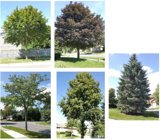
Figure 1.1: Study area for chapters 2 and 3 within London, Ontario. Sentinel-2 image used for city overview. ... 8 Figure 2.1: Study area within London, Ontario ... 18 Figure 2.2: Trees classified in study. Clockwise from top left: Norway maple, Schwedleri Norway maple, Colorado blue spruce, littleleaf linden, honey locust. ... 20 Figure 2.3: General workflow for creation of classification features. Features derived from imagery are in blue, from lidar in yellow. ... 21 Figure 2.4: Manual crowns (red) and generated crowns (green) ... 23 Figure 2.5: Selected tree crowns within the study area. ... 26 Figure 2.6: Process for extracting reflectance features: a) Geoeye-1 imagery with crown object overlying pixels. b) NDVI threshold, pixels over 0.5 NDVI in green, grey masked. c) NIR band, used for sunlit mask. d) Sunlit mask, pixels below mean NIR reflectance in crown masked out (grey). e) Remaining pixels after application of both masks. ... 28 Figure 2.7: a) Lidar points viewed from above, with outline of crown shown. Lidar features calculated only for points within crown object. b) Lidar point cloud viewed from side,

showing varying elevations of points. Points below 1.37 m excluded from calculations. ... 29 Figure 2.8: Data used to generate texture features, with example for each tree type. From top to bottom: nDSM, shaded relief, pansharpened Geoeye-1 imagery. Note that the tree crown object goes along edges of trees. For this reason, reduced sized objects were used for the calculation of texture features. ... 30 Figure 2.9: Features derived from Geoeye-1 imagery. Black: Texture features. Orange: Reflectance features (NDVI mask). Red: Reflectance features (Sunlit mask). ... 31 Figure 2.10: Features derived from lidar data. Black: Lidar height and intensity features from point cloud. Red: Texture features from lidar derived nDSM and shaded relief. ... 32

(11)

xi

Figure 2.11: Producer’s accuracy for all five tree types, when classified using different

groups of features. ... 46

Figure 2.12: User’s accuracy for all five tree types, when classified using different groups of features. ... 47

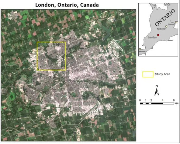
Figure 3.1: Location of study area (yellow) within London, Ontario. ... 59

Figure 3.2: Planetscope images used for classification. ... 63

Figure 3.3: VENuS images used for classification. ... 64

Figure 3.4: Planetscope spectral means for vegetation training classes. ... 73

Figure 3.5: VENuS spectral means for vegetation training classes. ... 74

Figure 3.6: Classification result using four-date Planetscope imagery... 77

Figure 3.7: Classification result using four-date VENuS imagery ... 78

Figure 3.8: Medway Creek and surrounding neighbourhood in four-date Planetscope and VENuS classifications ... 80

Figure 3.9: Four-date Planetscope and VENuS classifications of relatively new subdivision in North London, containing mostly small trees ... 80

(12)

xii

List of Appendices

Appendix A: Classification features used in chapter 2 ... 93

Appendix B: Confusion matrices for chapter 2 ... 98

Appendix C: Confusion matrices for chapter 3 ... 101

(13)

Chapter 1

1

Introduction

1.1 Importance of Urban Trees

From isolated trees along city streets to dense stands within parks, the urban forest is a prominent aspect of many cities. The urban forest refers to all woody vegetation within and around human settlements (Miller 1997). This includes individual trees on streets and in yards, woodlands of naturally growing trees, as well as plantations (Konijnendijk 2005). Urban forests provide numerous benefits to both the environment and the human population of cities. As they come from the natural functioning of an ecosystem, these benefits can be defined as ecosystem services (Carreiro, Song, and Wu 2008).

Ecosystem services include improvements to air quality, temperature, biodiversity, and human physical and mental health. Trees benefit air quality by removing pollutants and particulates which are trapped on the surface of the tree and absorbed into it (Carreiro, Song, and Wu 2008). Trees can also help reduce temperatures, which is a major concern due to urban heat effects. For example, parks are often 2-3 °C cooler than the surrounding city (Konijnendijk 2005). Shading also reduces the

temperature of buildings, therefore lowering cooling costs and energy use, while trees acting as wind buffers can reduce heating costs in winter (Carreiro, Song, and Wu 2008). From a broader climatic perspective, trees are also beneficial as they sequester carbon during their lifetimes, reducing the greenhouse effect (Carreiro, Song, and Wu 2008). Trees also improve biodiversity by providing habitat for other species. This is most significant with old, primary forest, but even individual trees provide habitat for birds and invertebrates (Konijnendijk 2005). There are also direct health benefits for humans. Access to urban forests can improve people’s physical health by encouraging them to go outside and be active. Even mental health may be improved, as trees have been tied to stress reduction (Konijnendijk 2005).

(14)

Not all trees provide these benefits equally. For example, a study of trees’ ability to trap particulates found differences based on size and species. Other trees may be unsuited to reducing pollution due to their intolerance to certain pollutants (Dawe 2011). In a park, the type of trees selected and their placement (e.g. individual trees or clusters of trees) will affect how people use the area around them (Konijnendijk 2005). The conditions that trees face also must be considered. Street trees will face more difficulties, such as polluted road runoff and higher wind stress, compared to trees in a denser

wooded area (Konijnendijk 2005). A diverse range of species is also important in order to minimize the impacts of pests or diseases that may target only a certain type of tree (Carreiro, Song, and Wu 2008). Tree biodiversity can also be considered an ecosystem service in its own right (Alvey 2006). Urban forests are often the location where non-native species are introduced and spread, but they also have the potential for high biodiversity (Alvey 2006). This is reflected within Ontario, with a number of cities in Southern Ontario establishing plans that support increasing the number of native tree species (Almas and Conway 2016).

1.2 Tree Classification Using Remote Sensing

Due to the benefits provided by trees, and the variations in these benefits between

species, it is necessary to have knowledge of tree species composition. It is one of the key components of urban tree inventories, along with factors such as determining tree size and condition (Miller 1997). Remote sensing can assist in obtaining this information. Older methods included making use of manual interpretation of aerial images to determine tree composition (Miller 1997). Now, a wide variety of data sources can be used as input for algorithms that are capable of classifying trees.

Remote sensing tree classification most commonly uses imagery (Fassnacht et al. 2016). Imagery is gathered by passive remote sensors, which measure electro-magnetic energy reflected of off objects in the area the sensor is monitoring. The sensor itself does not emit energy. The sensor typically contains multiple bands, which sense electro-magnetic energy from certain wavelength ranges. The number of bands differs between sensors. A sensor with more than 50 bands is defined as hyperspectral, more than 10 as superspectral and less than 10 (but still with multiple bands) as multispectral (Jones and

(15)

Vaughan 2010). A larger number of bands means that a difference that exists only in a small wavelength range may be detected by hyperspectral, but not with lower spectral resolution sensors. Vegetation, including trees, typically have similar reflectance patterns: low reflectance in blue and red wavelengths, somewhat higher reflectance in green

wavelength and much higher reflectance in near infrared wavelengths. Due to the similarities in reflectance, it is sometimes stated that hyperspectral is needed to

successfully differentiate vegetation (Alonzo, Bookhagen, and Roberts 2014). In recent years, studies classifying tree species using hyperspectral have become the most common (Fassnacht et al. 2016). However, there are still studies that achieve success using

multispectral sensors, albeit typically with lower numbers of classified species (Table 1.1).

(16)

Table 1.1: Past remote sensing studies on tree classification Year/Author Sensor # Band s Resolutio n (m) Object/ Pixel Classes

1998 Martin AVIRIS 224 20 Pixel 11 (Stands of species, mixed) 2003

Goodenough Hyperion 242 25 Pixel

10 (Species dominant, other landcover) 2003 Goodenough cont. Landsat-7 6 25 Pixel

10 (Species dominant, other landcover)

2004 Xiao AVIRIS 224 3.5 Pixel 16 (Species) 2010 Jones

AISA

Dual 492 2 Pixel 11 (Species) 2012 Cho

CAO

Alpha 288 1.12 Pixel 6 (Species) 2012 Cho cont. WorldVi ew 2 8 1.12 Pixel 6 (Species) 2012 Cho cont. Quickbir d 4 1.12 Pixel 6 (Species) 2012 Dalponte AISA Eagle 126 1 Pixel

8 (Species, other broadleaf, conifer, non-forest)

2012 Immitzer

WorldVi

ew 2 8 2 Object 10 (Species)

2012 Jensen AISA 248 2.2 Object 10 (Species, Genus) 2012 Zhang

AISA

Dual 492 1.6 Object 40 (Species) 2013 Adelabu

RapidEy

e 4 5 Pixel 5 (Species)

2013 Alonzo AVIRIS 224 3.7 Object 15 (Species) 2014 Alonzo AVIRIS 224 3.7 Object 29 (Species) 2016 Immitzer

Sentinel-2 13 10 Object 7 (Stands of species) 2017 Liu

CASI

1500 72 1 Object 15 (Species) 2017 Shen

AISA

Eagle 64 0.6 Object 5 (Species)

Spatial resolution is another major aspect of a passive sensor. Sensors have

different sized instantaneous fields of view, which is the angle in which energy is focused on the sensor. The ground-projected area of the instantaneous field of view determines the spatial resolution. In digital images, this will be the size of one pixel (Jensen 2005). A pixel will have values for each band, representing the measured energy for that area. All objects in that area will influence the value of the pixel. This leads to mixed pixels, in which a pixel represents multiple objects (e.g. multiple trees, tree and surrounding ground

(17)

cover). The size of the pixel can determine whether it is possible to separate individual trees. If the pixel size is too coarse to do so, classification may instead be based on pure stands of a single tree species, or mixtures of multiple tree species (Fassnacht et al. 2014). In contrast, higher resolution sensors allow for the classification of individual trees by species, whether for objects or for individual pixels.

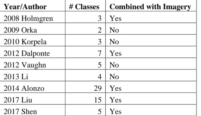
In addition to passive sensors, there are also active sensors which emit their own energy and measure its return. Examples include radar and lidar, of which lidar is more commonly used for classifying tree species (Fabian Ewald Fassnacht et al. 2016). Lidar emits laser pulses which are reflected off objects they hit, returning information about the elevation of the object, as well as the amount of returned energy. Further values can be derived from lidar, including numerous measures of tree structure. Lidar can be used on its own to classify tree species or be combined with imagery (Table 1.2).

Table 1.2: Past tree classification studies making use of lidar data

Year/Author # Classes Combined with Imagery 2008 Holmgren 3 Yes 2009 Orka 2 No 2010 Korpela 3 No 2012 Dalponte 7 Yes 2012 Vaughn 5 No 2013 Li 4 No 2014 Alonzo 29 Yes 2017 Liu 15 Yes 2017 Shen 5 Yes

Classification algorithms assign classes either to individual pixels (pixel-based classification) or to objects covering multiple pixels (object-based classification).

Classification can either be supervised, where image pixels/objects are compared to user-defined training areas, or unsupervised where the classifier automatically selects natural grouping within the image as classes. At the simplest level, classification is based on pixel values, with pixels/objects being assigned to the training class whose spectral values are closest to their own. (Jensen 2005). However, many different classification methods exist which have more complicated means of classification. Commonly used

(18)

parametric classifiers, which have assumptions that must be met about the distribution of data, include maximum likelihood classifier and linear discriminant analysis. However, it is becoming more common to use non-parametric methods which do not require

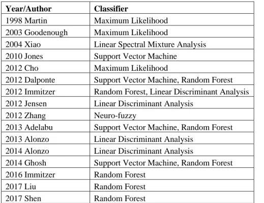
assumptions about data distribution (Plaza et al. 2017). Two commonly used methods are support vector machine and random forest (Table 1.3). This thesis focuses on support vector machine classification.

Table 1.3: Classification methods used in previous studies

Year/Author Classifier

1998 Martin Maximum Likelihood 2003 Goodenough Maximum Likelihood

2004 Xiao Linear Spectral Mixture Analysis 2010 Jones Support Vector Machine

2012 Cho Maximum Likelihood

2012 Dalponte Support Vector Machine, Random Forest 2012 Immitzer Random Forest, Linear Discriminant Analysis 2012 Jensen Linear Discriminant Analysis

2012 Zhang Neuro-fuzzy

2013 Adelabu Support Vector Machine, Random Forest 2013 Alonzo Linear Discriminant Analysis

2014 Alonzo Linear Discriminant Analysis

2014 Ghosh Support Vector Machine, Random Forest 2016 Immitzer Random Forest

2017 Liu Random Forest

2017 Shen Random Forest

Typically, numerous features are used for classification. The most basic feature is reflectance or pixel values from imagery. For trees, these values (and thus the light reflected off of trees) in related to chemical properties of leaves, the shape and structure of leaves and the shape and structure of the tree canopy (Fassnacht et al. 2016). Many additional classification features can be derived from image pixel values. From lidar, the height and reflected energy of laser points reflected off of trees can be used to derived numerous structural measures. This will be described in more detail in the following chapters.

(19)

1.3 Study Area and Data

This thesis focused on the urban forest of London, Ontario. As of the 2016 census, London had a population of 383,437 and an area of 232.48 km2 (Statistics Canada 2017). The urban forest of London is diverse, with trees in different settings including individual trees along streets, and natural forest in environmentally significant areas. London is also diverse in terms of species. The city is located in the Carolinian zone of Canada, the only primarily deciduous forest in the country. Many species found here are more common in the United States, and not present elsewhere in Canada (Almas and Conway 2016). Additionally, the inventory of city-maintained trees in London makes it clear that many introduced species are present.

The data used to classify the urban forest of London comes from several different sensors. Chapter 2 makes use of high-resolution multispectral Geoeye-1 imagery, as well as lidar data. Chapter 3 uses multispectral Planetscope imagery, and superspectral

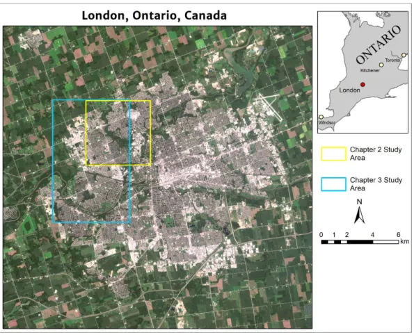
VENuS imagery, both of which have high spatial resolution, though lower than Geoeye-1. The extents of the study areas of both chapters are shown in the map below (Figure 1.1).

(20)

Figure 1.1: Study area for chapters 2 and 3 within London, Ontario. Sentinel-2 image used for city overview.

1.4 Research Objectives

This thesis focuses on further examining the potential of remote sensing for tree

classification. Although both methods draw on high resolution multispectral imagery, the exact circumstances vary. Chapter 2 focuses on higher quality, but less accessible data. Namely, Geoeye-1 imagery with 1.6 m resolution is used, alongside lidar data. Both datasets are capable of classifying individual trees at the species level. However, they are not easily obtained. Geoeye-1 is expensive, as are other sensors with similar spatial resolution. The lidar data is from an Ontario government initiative and is publicly available, but repeated coverage of the same area on different dates is not available. In contrast, chapter 3 focuses on imagery with somewhat lower resolution (3 m and 5 m for Planetscope and VENuS respectively). This is still quite high but is too coarse to resolve

(21)

most individual trees. These sensors instead benefit from repeated observations of the same area, allowing images from multiple seasons to be used for classification. The research goals of this thesis are mostly focused on specific chapters. The goals of chapter 2 are:

1) Identify which features from high-resolution multispectral imagery and lidar data contribute most to accurately classifying tree species.

2) Determine if combining high-resolution multispectral imagery and lidar results in a higher classification accuracy than either data source can achieve individually.

The goals for chapter 3 are:

3) Assess the ability of multitemporal classification using Planetscope and VENuS to improve the classification of vegetation.

4) Identify which image dates and combinations of dates are best suited to distinguishing vegetation classes.

Chapter 2 involves classifying five different types of trees at the object level, while making use of classification features from high-resolution imagery and lidar data. This combination is common in past research and in general results in a more accurate classification than either source of data can provide on its own. The main purpose of the study is to examine features from imagery and lidar in more detail, testing features that have been used in past studies but rarely all used at one time. In some cases, more variations have been used, such as generating texture measures for all spectral bands rather than only certain bands.

Chapter 3 focuses on multitemporal classification, using multiple images from the same sensor of the same area at different times of the year for classification. This has been tested for various sensors in the past, with accuracy typically higher for

classification using multiple image dates. However, the sensors used in this chapter, Planetscope and VENuS, are fairly new and have not yet been used for tree classification using multidate imagery.

(22)

1.5 Thesis Organization

This thesis uses integrated article format. Chapter 1 provides background information on the urban forest and tree classification using remote sensing and presents the research objectives. Chapter 2 examines object-based tree species classification using both high-resolution multispectral imagery and lidar data. Chapter 3 details pixel-based

multitemporal classification of landcover, including two types of trees (deciduous and coniferous). Chapter 4 summarizes the findings of chapters 2 and 3.

1.6 References

Adelabu, Samuel, Onisimo Mutanga, Elhadi Adam, and Moses Azong Cho. 2013. “Exploiting Machine Learning Algorithms for Tree Species Classification in a Semiarid Woodland Using RapidEye Image.” Journal of Applied Remote Sensing 7 (1): 073480. doi:10.1117/1.JRS.7.073480.

Almas, Andrew D., and Tenley M. Conway. 2016. “The Role of Native Species in Urban Forest Planning and Practice: A Case Study of Carolinian Canada.” Urban Forestry and Urban Greening 17. Elsevier GmbH.: 54–62. doi:10.1016/j.ufug.2016.01.015.

Alonzo, Michael, Bodo Bookhagen, and Dar A. Roberts. 2014. “Urban Tree Species Mapping Using Hyperspectral and Lidar Data Fusion.” Remote Sensing of Environment 148. Elsevier Inc.: 70–83. doi:10.1016/j.rse.2014.03.018.

Alonzo, Mike, Keely Roth, and Dar Roberts. 2013. “Identifying Santa Barbara’s Urban Tree Species from AVIRIS Imagery Using Canonical Discriminant Analysis.” Remote Sensing Letters 4 (5): 513–521. doi:10.1080/2150704X.2013.764027.

Alvey, Alexis A. 2006. “Promoting and Preserving Biodiversity in the Urban Forest.” Urban Forestry and Urban Greening 5 (4): 195–201. doi:10.1016/j.ufug.2006.09.003.

(23)

Carreiro, Margaret, Yong-Chang Song, and Jianguo Wu. 2008. Ecology, Planning, and Management of Urban Forests. Springer.

Cho, Moses Azong, Renaud Mathieu, Gregory P. Asner, Laven Naidoo, Jan van Aardt, Abel Ramoelo, Pravesh Debba, et al. 2012. “Mapping Tree Species Composition in South African Savannas Using an Integrated Airborne Spectral and LiDAR System.” Remote Sensing of Environment 125. Elsevier Inc.: 214–226. doi:10.1016/j.rse.2012.07.010. Dalponte, Michele, Lorenzo Bruzzone, and Damiano Gianelle. 2012. “Tree Species Classification in the Southern Alps Based on the Fusion of Very High Geometrical Resolution Multispectral/Hyperspectral Images and LiDAR Data.” Remote Sensing of Environment 123. Elsevier Inc.: 258–270. doi:10.1016/j.rse.2012.03.013.

Dawe, Gerald. 2011. The Routledge Handbook of Urban Ecology. Edited by Ian Douglas, David Goode, Michael Houck, and Rusong Wang. New York: Routledge. Fassnacht, Fabian E., Carsten Neumann, Michael Forster, Henning Buddenbaum, Aniruddha Ghosh, Anne Clasen, Pawan Kumar Joshi, and Barbara Koch. 2014. “Comparison of Feature Reduction Algorithms for Classifying Tree Species with Hyperspectral Data on Three Central European Test Sites.” IEEE Journal of Selected Topics in Applied Earth Observations and Remote Sensing 7 (6): 2547–2561.

doi:10.1109/JSTARS.2014.2329390.

Fassnacht, Fabian Ewald, Hooman Latifi, Krzysztof Stereńczak, Aneta Modzelewska, Michael Lefsky, Lars T. Waser, Christoph Straub, and Aniruddha Ghosh. 2016. “Review of Studies on Tree Species Classification from Remotely Sensed Data.” Remote Sensing of Environment 186: 64–87. doi:10.1016/j.rse.2016.08.013.

Ghosh, Aniruddha, Fabian Ewald Fassnacht, P. K. Joshi, and Barbara Kochb. 2014. “A Framework for Mapping Tree Species Combining Hyperspectral and LiDAR Data: Role of Selected Classifiers and Sensor across Three Spatial Scales.” International Journal of Applied Earth Observation and Geoinformation 26 (1). Elsevier B.V.: 49–63.

(24)

Goodenough, David G., Andrew Dyk, K. Olaf Niemann, Jay S. Pearlman, Hao Chen, Tian Han, Matthew Murdoch, and Chris West. 2003. “Processing Hyperion and ALI for Forest Classification.” IEEE Transactions on Geoscience and Remote Sensing 41 (6 PART I): 1321–1331. doi:10.1109/TGRS.2003.813214.

Holmgren, J., Å Persson, and U. Söderman. 2008. “Species Identification of Individual Trees by Combining High Resolution LiDAR Data with Multi-Spectral Images.” International Journal of Remote Sensing 29 (5): 1537–1552.

doi:10.1080/01431160701736471.

Immitzer, Markus, Francesco Vuolo, and Clement Atzberger. 2016. “First Experience with Sentinel-2 Data for Crop and Tree Species Classifications in Central Europe.” Remote Sensing 8 (3). doi:10.3390/rs8030166.

Jensen, John. 2005. Introductory Digital Image Processing: A Remote Sensing Perspective. 3rd ed. Upper Saddle River, N.J.: Pearson Prentice Hall.

Jensen, Ryan R., Perry J. Hardin, and Andrew J. Hardin. 2012. “Classification of Urban Tree Species Using Hyperspectral Imagery.” Geocarto International 27 (5): 443–458. doi:10.1080/10106049.2011.638989.

Jones, Hamlyn, and Robin Vaughan. 2010. Remote Sensing of Vegetation: Principles, Techniques, and Applications. Oxford: Oxford University Press.

Jones, Trevor G., Nicholas C. Coops, and Tara Sharma. 2010. “Assessing the Utility of Airborne Hyperspectral and LiDAR Data for Species Distribution Mapping in the Coastal Pacific Northwest, Canada.” Remote Sensing of Environment 114 (12). Elsevier Inc.: 2841–2852. doi:10.1016/j.rse.2010.07.002.

Konijnendijk, Cecil C. 2005. Urban Forests and Trees. Edited by Cecil Konijnendijk, Kjell Nilsson, Thomas Randrup, and Jasper Schipperijn. Urban Forests and Trees. Berlin, Heidelberg: Springer Berlin Heidelberg. doi:10.1007/3-540-27684-X.

Korpela, Ilkka, Hans Ole Ørka, Matti Maltamo, Timo Tokola, and Juha Hyyppä. 2010. “Tree Species Classification Using Airborne LiDAR - Effects of Stand and Tree

(25)

Parameters, Downsizing of Training Set, Intensity Normalization, and Sensor Type.” Silva Fennica 44 (2): 319–339. doi:10.14214/sf.156.

Li, Jili, Baoxin Hu, and Thomas L. Noland. 2013. “Classification of Tree Species Based on Structural Features Derived from High Density LiDAR Data.” Agricultural and Forest Meteorology 171–172. Elsevier B.V.: 104–114. doi:10.1016/j.agrformet.2012.11.012. Liu, Luxia, Nicholas C. Coops, Neal W. Aven, and Yong Pang. 2017. “Mapping Urban Tree Species Using Integrated Airborne Hyperspectral and LiDAR Remote Sensing Data.” Remote Sensing of Environment 200 (July). Elsevier: 170–182.

doi:10.1016/j.rse.2017.08.010.

Martin, M.E, S.D Newman, J.D Aber, and R.G Congalton. 1998. “Determining Forest Species Composition Using High Spectral Resolution Remote Sensing Data.” Remote Sensing of Environment 65 (3): 249–254. doi:10.1016/S0034-4257(98)00035-2.

Miller, Robert. 1997. Urban Forestry: Planning and Managing Urban Greenspaces. Upper Sadle River, N.J.: Prentice-Hall.

Ørka, Hans Ole, Erik Næsset, and Ole Martin Bollandsås. 2009. “Classifying Species of Individual Trees by Intensity and Structure Features Derived from Airborne Laser Scanner Data.” Remote Sensing of Environment 113 (6). Elsevier Inc.: 1163–1174. doi:10.1016/j.rse.2009.02.002.

Plaza, Antonio J, Pedram Ghamisi, Javier Plaza, Yushi Chen, and Jun Li. 2017.

“Advanced Spectral Classifiers for Hyperspectral Images: A Review.” IEEE Geoscience and Remote Sensing Magazine 5 (1): 8–32. doi:10.1109/mgrs.2016.2616418.

Shen, Xin, and Lin Cao. 2017. “Tree-Species Classification in Subtropical Forests Using Airborne Hyperspectral and LiDAR Data.” Remote Sensing 9 (11).

doi:10.3390/rs9111180.

Statistics Canada. 2017. London [Population centre], Ontario and Ontario [Province] (table). Census Profile. 2016 Census. Statistics Canada Catalogue no. 98-316-X2016001. Ottawa. Released November 29, 2017.

(26)

https://www12.statcan.gc.ca/census-recensement/2016/dp-pd/prof/index.cfm?Lang=E Vaughn, Nicholas R., L. Monika Moskal, and Eric C. Turnblom. 2012. “Tree Species Detection Accuracies Using Discrete Point Lidar and Airborne Waveform Lidar.” Remote Sensing 4 (2): 377–403. doi:10.3390/rs4020377.

Xiao, Q., S. L. Ustin, and E. G. McPherson. 2004. “Using AVIRIS Data and Multiple-Masking Techniques to Map Urban Forest Tree Species.” International Journal of Remote Sensing 25 (24): 5637–5654. doi:10.1080/01431160412331291224.

Zhang, Caiyun, and Fang Qiu. 2012. “Mapping Individual Tree Species in an Urban Forest Using Airborne Lidar Data and Hyperspectral Imagery.” Photogrammetric Engineering & Remote Sensing 78 (10): 1079–1087. doi:10.14358/PERS.78.10.1079.

(27)

Chapter 2

2

Tree Species Classification Using High-resolution

Multispectral Imagery and Lidar

2.1 Introduction

2.1.1 Tree Classification Data Sources

Urban trees provide numerous benefits to cities. These include social benefits such as improving the aesthetic appeal of cities, as well as physical benefits like

controlling urban heat and air pollution (Konijnendijk 2005). However, many trees within cities are introduced species, which may not aid the proper functioning of the local

ecosystem. Increasing the proportion of native tree species within cities is already a target for certain municipalities in Southern Ontario (Almas and Conway 2016). Assessing tree species diversity is also a common goal of tree inventories carried out by cities. However, conducting inventories is expensive and time consuming (Östberg et al. 2013).

Identifying species using remote sensing can provide a solution, as it is faster than ground surveys, and potentially more cost effective (Fassnacht et al. 2016).

Both spectral imagery and lidar data have been used to successfully identify tree species. Spectral imagery differentiates tree species on the basis on reflectance

differences between species, which are influenced by chemical properties as well as leaf morphology and canopy structure (Fassnacht et al. 2016). Due to the similarity in

reflectance between species, this is often performed using hyperspectral sensors (Alonzo, Bookhagen, and Roberts 2014). Hyperspectral sensors measure reflected light using a large number of bands measuring narrow wavelength ranges. In contrast, multispectral sensors measure light using a small number of bands covering large wavelength ranges. However, a number of studies have used multispectral sensors and achieved some success when classifying trees (Goodenough et al. 2003, Immitzer, Atzberger, and Koukal 2012, Adelabu et al. 2013). Cho et al. 2012 found that hyperspectral and four-band Quickbird imagery achieved almost identical overall accuracy.

(28)

Lidar functions by emitting laser pulses, which are reflected back to the sensor from objects. Returned lidar pulses contain information on elevation and returned energy. Numerous lidar features can be created from this information, but ultimately they

represent the structure of the crown and foliage (Fassnacht et al. 2016). Intensity, representing reflected energy from the laser (often infrared), is associated both with leaf reflectance and structure (Korpela et al. 2010). Lidar data is also capable of tree

classification, although studies using solely lidar data generally identify only a few key species (Ørka, Næsset, and Bollandsås 2009, Korpela et al. 2010, Vaughn, Moskal, and Turnblom 2012, Shi et al. 2018).

The combination of spectral and lidar data can better classify tree species than either data source can individually. Increases in overall accuracy when comparing classification using hyperspectral data alone to classification using hyperspectral and lidar data include Dalponte et al. 2012 (6 species and non-forest, 74.1% to 84%), Alonzo et al. 2014 (29 species, 79.2% to 83.4%) and Shen 2017 (5 classes, 88.8% to 90.6%). An especially large increase was Liu 2017 with an increase from 51.1% to 70% with 15 species. The large increase was attributed to the early stage of leaf growth making lidar more useful than spectral data (Liu et al. 2017). Similar improvements were found in studies using multispectral images and lidar such as Holmgren et al. 2008 (3 classes, 84% to 94%) and Ke et al. 2010 (5 species dominant stand classes, 84 kappa to 92 kappa).

2.1.2 Classification Features

Classification features derived from spectral images most commonly include the pixel values or reflectance of the sensor’s bands. For object based classification, the mean of the pixels in tree crowns is often used (Fassnacht et al. 2016). Limiting the calculation of the mean to the brightest pixels in the crown has been found to improve accuracy (Shen and Cao 2017). Alternatively, a single pixel from the top of the tree crown may be selected (Zhang and Qiu 2012).

Lidar features generally represent crown density, shape, and surface texture, as well as return intensity (Vaughn, Moskal, and Turnblom 2012). Features based on the height of lidar points include exact heights of points (e.g. maximum height), statistics

(29)

calculated from those heights (e.g. mean, skew and kurtosis of height), and percentiles (e.g. height which 95% of lidar points in crown fall below).

The utility of height features varies between studies. Ørka et al. 2009, Vaughn et al. 2012 and Korpela et al. 2010 all found intensity measures to be more useful than height measures. In contrast, Ke et al. 2010 found height useful when classifying natural forest, and Cho et al. 2012 found a 5.8 percentage point increase in overall accuracy when using maximum height alongside spectral data to classify savannah trees.

Image texture refers to the image being rough or smooth. In digital images, it is based on the differences between pixel values (Hall-Beyer 2018). The inclusion of texture improves image classification (Coburn and Roberts 2004). Texture measures can be derived from either the spectral image or a lidar product such as a normalized digital surface model (nDSM). Common measures used include grey level co-occurrence matrix textures (GLCM) which are based on different grey-level combinations within a moving window (Hall-Beyer 2018). Their usefulness varies, with Li et al. 2015 finding them less useful than spectral features, while in Heinzel et al. 2012 GLCM measures from both imagery and nDSM were among the 14 most important features in the study.

2.1.3 Research Objectives

The purpose of this study was to better understand the ability of imagery and lidar to classify tree species. This was accomplished by making use of numerous classification features derived from both high-resolution multispectral imagery and lidar. These

included spectral means, texture measures of imagery and a normalized digital surface model, and measures of lidar height and intensity. The overall goals of the study were: 1) Achieve an accurate classification of five types of trees in London, Ontario using support vector machine classification with features derived from high-resolution multispectral Geoeye-1 imagery and lidar.

2) Identify which classification features contribute most to the accuracy of the classification result.

(30)

3) Verify if combining high-resolution multispectral imagery and lidar results in a higher classification accuracy than either data source can achieve individually.

2.2 Methodology

2.2.1 Study Area and Data Description

London, Ontario is located in southern Ontario, Canada. The city contains isolated urban trees along streets and on private property, as well as denser clusters of trees within parks and environmentally significant areas. The study area covers approximately 25 km2 in the north of London, corresponding to the boundary of the study’s Geoeye-1 image. This area contains both new and old neighbourhoods, leading to a variety of tree ages and sizes (Figure 2.1)

(31)

The study made use of a Geoeye-1 image captured on July 9, 2018. Geoeye-1 is a satellite mounted high-resolution multispectral sensor owned by the company

DigitalGlobe. The satellite is in sun-synchronous orbit at 684 km and makes 12 to 13 orbits daily. It contains four bands corresponding to blue, green, red and near-infrared (NIR) wavelengths (Table 2.1). The multispectral bands have a spatial resolution of 1.6 m. Additionally, there is a panchromatic band with a spatial resolution of 0.4 m.

Table 2.1: Geoeye-1 imagery specifications

Band # Wavelength (nm) Colour Spatial Resolution (m)

Band 1 450-510 Blue 1.6

Band 2 510-580 Green 1.6

Band 3 655-690 Red 1.6

Band 4 780-920 Near Infrared 1.6

Panchromatic 450-800

Greyscale (covers visible spectrum to beginning of

NIR) 0.4

The study’s lidar data was collected on May 15, 2017 using an aircraft mounted Leica ALS70-HP. This sensor is produced by Leica Geosystems. The study area data is part of a larger lidar dataset of Southwestern Ontario around Lake Erie and is collected and provided by the Ministry of Agriculture, Food and Rural Affairs (OMAFRA). The average lidar point density is 8 points/m2 _{and the wavelength of the laser is 1064 nm.} Each lidar pulse may have up to five returns.

2.2.2 Class Selection

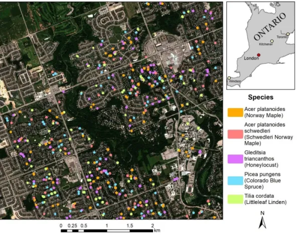
There are numerous tree species in the study area, both native and introduced. The city’s tree inventory accounts for many city-maintained trees, including most street trees and some park trees. Within the study area, this includes over 160 species. Classification was performed to differentiate between five tree types. Four species were selected: Acer platanoides (Norway maple), Tilia cordata (littleleaf linden), Picea pungens (Colorado blue spruce)and Gleditsia triacanthos (honey locust). In addition, the Norway maple cultivar “Schwedleri” was also selected. These species are among the ten most common in the study area, according to the city tree inventory. However, they are also all

(32)

marked physical differences. Colorado blue spruce is the only conifer of the five and has blue-green coloured needles. The leaf and crown shapes of Norway maple, littleleaf linden and honey locust are all distinct. Norway maple and Schwedleri Norway maple have the same crown and leaf shape, but “Schwedleri” is distinguished by red coloured foliage (Figure 2.2).

Figure 2.2: Trees classified in study. Clockwise from top left: Norway maple, Schwedleri Norway maple, Colorado blue spruce, littleleaf linden, honey locust.

2.2.3 Workflow

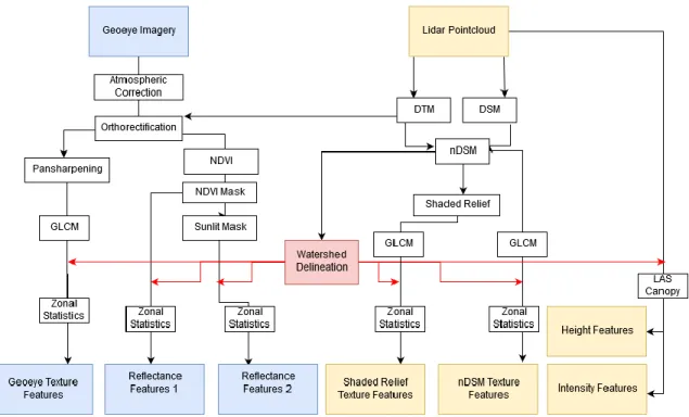
The general stages of processing are shown in the flowchart below (Figure 2.3).

Classification began with preprocessing Geoeye imagery through atmospheric correction and orthorectification. The lidar point cloud was also processed to generate elevation

(33)

products including a normalized digital surface model (nDSM). The nDSM was the basis of watershed delineation, which created the tree crown objects used in the study. Shaded relief elevation images were also created from the nDSM. The Geoeye image was further processed by pansharpening (increasing resolution to panchromatic band pixel size of 0.4 m). The pansharpened bands were used to generate GLCM texture measures.

Additionally, GLCM textures were generated from the nDSM and four shaded relief images. The original 1.6 m Geoeye bands were masked based on NDVI and bright pixels (sunlit) to ensure only tree vegetation reflectance was measured. From these new images (masked Geoeye images, GLCM texture for pansharpened Geoeye bands, shaded relief and nDSM) zonal statistics in ArcGIS was run to calculate features from the pixels in the tree crown object. Additionally, LAS Canopy was used to calculate metrics from the lidar points within the tree crown object boundaries. This provided all the features used for classification in this study. More detailed explanations for each stage are provided in the following subsections.

Figure 2.3: General workflow for creation of classification features. Features derived from imagery are in blue, from lidar in yellow.

(34)

2.2.4 Object Creation

This study used object-based classification, where pixels representing the same feature are grouped together as an object and assigned the same class. Here, the objects represent individual tree crowns. Segmentation of tree crown objects was performed using marker-controlled watershed segmentation from the R Forest Tools package (Plowright 2018).

The algorithm delineates tree crowns from an nDSM, which represents the height of objects as if they were on a level plane, without the influence of terrain elevation. The nDSM was generated from lidar. A digital surface model (DSM) was generated based on the highest elevation lidar point for each cell, while a digital terrain model (DTM) was generated based on the average elevation of ground lidar points in each cell. The DTM was then subtracted from the DSM to obtain the nDSM.

Marker controlled watershed segmentation uses a search window to find local maxima and delineates the “watershed” around them. Here, the local maxima represent the tops of trees. Tree crowns tend to increase in size alongside tree height. A more accurate segmentation can be achieved by changing the size of the search window in relation to the elevation value of the pixel (Chen et al. 2006). To establish how crown size varies with height, 105 trees of several common species were manually delineated. Their maximum height and crown width were recorded and a curve was plotted through these points to establish a function between tree height and crown size (Chen et al. 2006). This resulted in under-segmentation, with several smaller crowns being merged together. To avoid this problem, a new function was generated using only the smallest crown for each 1 m height interval.

Segmentation was performed using three nDSMs of various pixel sizes (1 m, 1 m with low-pass filter, 0.5 m, 0.5 m with low-pass filter). The low-pass filter was used to fill gaps and irregularities in crowns, which were particularly noticeable in the 0.5 m image (Barnes et al. 2017). The unfiltered 0.5 raster produced poor results and was not further analyzed. From visual examination, height differences between crowns were

(35)

noticeable at both resolutions, but differences within crowns were emphasized more strongly with 0.5 m pixel size.

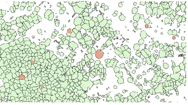
The generated crowns were compared to manually delineated crowns to determine segmentation quality (Figure 2.4). The sections of generated crowns that intersected manual crowns were extracted, with each containing three measurements of area: the area of the manual crown, the area of the original generated crown, and the area of the section of the generated crown that intersects the manual crown.

Figure 2.4: Manual crowns (red) and generated crowns (green)

Three metrics for segmentation quality were then created:

1) The total number of generated crowns that intersect a manual crown. The number of intersecting generated crowns should be lower, as that indicates a single manual crown is not split between multiple generated crowns.

2) For each manual crown, the largest intersecting generated crown area divided by the total area of intersecting generated crowns. If there are multiple intersecting crowns, it is preferable that a single one cover most of the manual crown. 3) The area of the section of a generated crown that intersects a manual crown,

(36)

generated crown intersecting the manual crown will be a similar size to the entire generated crown. If not, it indicates that multiple tree crowns are contained in the generated crown.

The metrics indicated that the low-pass filtered 0.5 m nDSM produced the best segmentation (Table 2.2). The 1 m low-pass filtered nDSM had fewer total intersecting generated crowns, indicating that single manual crowns were not split between multiple generated objects. However, the size of the part of the generated object that intersects with the manual crown was much smaller than the total size of that object, suggesting that the generated object represents multiple tree crowns. In contrast, the 0.5 m low-pass filtered nDSM, generated objects more often contained only a single tree crown. On average, the intersecting area of the generated object containing the manual crown made up 73.76% of the total area of the same generated object. Because of the higher quality of crowns based on the measurements, further processing made use of the objects generated by the 0.5 m low-pass filtered nDSM.

Table 2.2: Accuracy measures for tree crown objects. Best value in green. LP = low-pass filter. Metric 1 is the exact value, metric 2 is mean of values for all generated crowns that intersect a watershed object, metric 3 is mean of values for largest intersecting generated crown for each manual crown.

2.2.5 Selection of Crowns for Classification

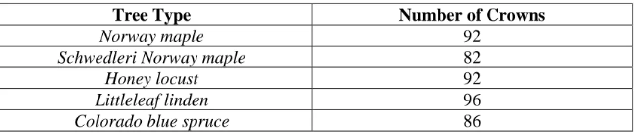
From the objects generated from watershed segmentation, 448 objects representing individual tree crowns were selected for classification (Table 2.3). The crowns represent trees of different ages and sizes throughout the study area. Because tree age can affect lidar intensity, an attempt was made to use trees of different ages for classification

nDSM Total # intersecting generated objects Largest generated object as percent of all intersecting objects

Area of generated object intersecting with manual crown / Area of entire generated object 1m 130 88.89% 71.61% 1m LP 102 96.45% 59.93% 0.5m LP 112 94.27% 73.76%

(37)

(Korpela et al. 2010). The study area was divided into nine sections, based on the typical size of trees. Within each section, 55 points (11 points per tree type) were placed

randomly. The nearest object of that point’s target tree species was selected to be used in classification. The species was verified using Google Streetview images. Selection was limited to city-maintained trees identified by the city inventory, and only objects

containing a single tree crown were used. This was to avoid confusion caused by a single object containing multiple trees of different species. However, it does mean that

classification accuracy is likely higher than if all tree crowns in the study area were classified. In some cases, there was no tree near the random point, so the exact number of sample crowns differs between species. Selected crowns were distributed throughout the study area, but limited to mostly to residential areas (Figure 2.5)

Table 2.3: Number of crowns selected for classification per tree type.

Tree Type Number of Crowns

Norway maple 92

Schwedleri Norway maple 82

Honey locust 92

Littleleaf linden 96

(38)

Figure 2.5: Selected tree crowns within the study area.

2.2.6 Image Processing

Further processing was required to generate the features used for classification from the imagery and lidar data. The Geoeye-1 image was provided without atmospheric

correction or orthorectification. ATCOR atmospheric correction was performed in PCI Geomatica to remove atmospheric distortion in the image and transform pixel values into surface reflectance (ATCOR Ground Reflectance Tutorial). Additionally,

orthorectification was performed using ENVI to adjust for distortion caused by elevation changes in the image, and to align properly with the tree crown objects and the nDSM from which they were delineated (Harris Geospatial. RPC Orthorectification Tutorial). Pansharpening was also performed, to enhance the resolution of multispectral Geoeye bands to that of the panchromatic resolution (0.4 m). This was done using the SPEAR pansharpening method in ENVI (Harris Geospatial. SPEAR Pansharpening).

(39)

From the Geoeye image, the mean and standard deviation (SD) for each of the four bands were found for each crown. Mean and SD were also calculated based on the normalized difference vegetation index (NDVI). NDVI is based on the difference between red and NIR band values and indicates healthy vegetation. The calculation was based on pixels that fall within the crown object. However, differing pixel sizes between the nDSM and the Geoeye image, as well as imperfect registration, meant that tree crown objects did not perfectly align with trees in the Geoeye image. Pixels representing other features would be included in metrics based on imagery. To avoid this problem, two masks were used. First, an NDVI mask was used to eliminate non-vegetation pixels. Pixels with a value below 0.5 were changed to no data, in order to avoid their inclusion when calculating metrics. Due to the high image resolution, there were large differences in pixel values within tree crowns caused by shadows. Past studies have indicated that selecting only sunlit pixels improves tree species classification (Immitzer, Atzberger, and Koukal 2012, Shen and Cao 2017). Once non-vegetation pixels were removed, a further mask was created by finding the mean NIR reflectance value of each crown, then

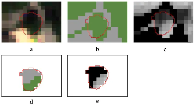
changing all pixels falling below that value to no data (Figure 2.6). The remaining pixels were considered sunlit. (Shen and Cao 2017). The mean and SD were calculated twice, once with only the NDVI mask applied, and a second time with the sunlight mask applied as well. This was performed using the zonal statistics tool in ArcGIS, which finds a mean value based on pixels within a polygon (ESRI).

(40)

Figure 2.6: Process for extracting reflectance features: a) Geoeye-1 imagery with crown object overlying pixels. b) NDVI threshold, pixels over 0.5 NDVI in green, grey masked. c) NIR band, used for sunlit mask. d) Sunlit mask, pixels below mean NIR reflectance in crown masked out (grey). e) Remaining pixels after application of both masks.

2.2.7 Lidar Processing

Lidar features were created in LASTools software, with the use of LASCanopy

(Rapidlasso). For each crown, the metrics were calculated based on lidar points within the bounds of the polygon (Figure 2.7). Points classified as ground or high/low noise were excluded, as were points which fell below a certain height (here left as the default value of 1.37 m). For both height and intensity, the same features were generated. These included exact values (minimum and maximum value of lidar points), statistics (mean, average square value, kurtosis, skewness, standard deviation) and percentiles. Height percentiles indicate that a certain percentage of lidar points fall below a certain height. Height percentiles were normalized to allow trees of different heights to be more directly comparable (e.g. 75% of points fall below 86% of the tree’s maximum height, rather than 7.8 m) (Ørka, Næsset, and Bollandsås 2009). Intensity percentiles indicate that a certain

(41)

percentage of points have an intensity value lower than a certain value (e.g. 75% of points have an intensity value of less than 25000).

Figure 2.7: a) Lidar points viewed from above, with outline of crown shown. Lidar features calculated only for points within crown object. b) Lidar point cloud viewed from side, showing varying elevations of points. Points below 1.37 m excluded from calculations.

2.2.8 Texture Processing

Texture measures were generated using the TEX algorithm in PCI Geomatica (PCI Geomatics. TEX Texture Analysis). The window for texture calculation was set as 3x3 due to the presence of small trees with relatively few pixels comprising the crown. Eight GLCM measures, and four GLDV measures were calculated. The grey level

co-occurrence matrix is created from pairs of pixel values between neighbouring pixels, while GLDV is based on the diagonal of the matrix (Hall-Beyer 2018). Textures were calculated based on the nDSM and all four Geoeye pansharpened bands.

Texture measures were also generated based on shaded relief images. Shaded relief is a visualization method that simulates the shadowing effect caused by differences in elevation and is typically used to represent surface roughness of terrain. In this study, the shadowing effect was instead used to exaggerate differences in pixel values of the nDSM for tree crowns. Shaded relief images for the four cardinal directions were

(42)

generated in ArcGIS using the nDSM, with sun azimuth at 0, 90, 180 and 270 degrees, and sun elevation at 45 degrees (Figure 2.8) Zonal statistics in ArcGIS was once again used to get a mean value for each texture measure. However, edges of trees had values that were influenced by the pixels surrounding the tree crown, rather than within crown pixel value differences. To exclude these, the tree crown polygons were decreased in size by 0.5 m on all sides (the size of one nDSM pixel).

Figure 2.8: Data used to generate texture features, with example for each tree type. From top to bottom: nDSM, shaded relief, pansharpened Geoeye-1 imagery. Note that the tree crown object goes along edges of trees. For this reason, reduced sized objects were used for the calculation of texture features.

In total, 160 classification features for each tree crown were generated (Figure 2.9 and Figure 2.10). For full descriptions of these features, see Appendix A.

(43)

Figure 2.9: Features derived from Geoeye-1 imagery. Black: Texture features. Orange: Reflectance features (NDVI mask). Red: Reflectance features (Sunlit mask).

(44)

Figure 2.10: Features derived from lidar data. Black: Lidar height and intensity features from point cloud. Red: Texture features from lidar derived nDSM and shaded relief.

(45)

2.2.9 Support Vector Machine Classification

Classification was performed using support vector machine (SVM) which is a machine learning classifier. SVM finds the best fitting hyperplane to separate two classes. Typically, a linear separation is not possible, so the data is transformed to a higher dimension where a separation can be made. This requires the use of a kernel, such as the radial basis function which is used in this study. Additionally, SVM is a binary classifier for separating two classes, so various methods have been developed to allow multiclass classification (Pu 2017). This study used the SVM implementation in the R package “e1071”, which uses the one-against-one technique (Meyer 2019). For each feature to be classified this method tries all possible binary combinations of classes and assigns the feature to the class which it is most often placed in (Gidudu, Hulley, and Marwala 2007).

SVM has several benefits for classification. In this study 160 features were tested, with up to 88 being used at a time, while only 448 tree crowns were available as training and testing data. With SVM, classification accuracy is not negatively affected by high dimensionality (Pu 2017). Additionally, it can perform well with a relatively small amount of training data (Fassnacht et al. 2016). The use of random forest classification was also considered, but ultimately SVM was chosen as it performed better in several tree classification studies (Immitzer, Atzberger, and Koukal 2012, Dalponte, Bruzzone, and Gianelle 2012, Adelabu et al. 2013, Shang and Chisholm 2014).

Once classification was performed, the results were compared to the true classes of the testing data. From the comparison of predicted and actual classes, a confusion matrix was generated (Table 2.4). Each column of the matrix shows what the training data was classified as. The mean of each column is the producer’s accuracy of the class, indicating how many testing samples were classified correctly for a particular class. The rows show to which class members of a predicted class truly belong. The mean of each row is the user’s accuracy. The sum of the diagonals divided by the total number of samples gives the overall accuracy, representing the percent of testing samples classified correctly (Lillesand, Kiefer, and Chipman 2008).

(46)

Table 2.4: Example confusion matrix. Classes A through E. Columns indicate the reference classes, while rows indicate the predicted classes. Column total is

producer’s accuracy for that class, row is user’s accuracy. Overall accuracy in red is the sum of the diagonals divided by the total number of samples

A B C D E Total UA A 71 19 2 2 2 96 0.739583 B 13 56 2 0 5 76 0.736842 C 4 3 86 0 5 98 0.877551 D 1 0 0 84 0 85 0.988235 E 3 4 2 0 84 93 0.903226 Total 92 82 92 86 96 448 PA 0.771739 0.682927 0.934783 0.976744 0.875 0.850446

In order to have better confidence in the results, five-fold cross validation was used. This method involves splitting the data into five groups, with the classes distributed evenly between the groups. Classification is run five times, using four groups as training data and one group as testing data. Each of the five groups is used once as testing data. The final overall accuracy (OA) is the mean of the overall accuracy from the five iterations (Rodríguez, Pérez, and Lozano 2010).

Initially, classification was performed with single features. This was to determine which were most useful for classification and guide the selection features to group

together later on. Each of the 160 features were used as the sole classification feature, and the resulting overall accuracy was recorded. Next, groups of related features were tested. The different combinations of features were based on the data source, the type of feature, and the results of single feature classification (e.g. removing low performing features). Following this, the best results of group classification were combined. In total, 75 different combinations of features were tested. The main groups of features are as follows:

1) Imagery pixel values 2) Imagery texture measures 3) nDSM texture measures

(47)

4) shaded relief texture measures 5) lidar height features

6) lidar intensity features.

2.3 Results

2.3.1 Single Feature Results

Intensity features performed far better than features from any other group (Table 2.5). The top seven most accurate single feature classification results came from intensity metrics. The 75th percentile of intensity had the highest classification accuracy at

63.42%, which outperforms entire groups of features (i.e. Geoeye reflectance, height features, nDSM texture). Other intensity features with high accuracy included statistical metrics (mean, skew and standard deviation) as well as middle range percentiles (25th – 90th). Percentiles at the upper and lower ends were less useful, as was the minimum intensity value. The maximum and 99th percentile of intensity were almost always the same value, and of no use for distinguishing species.

Table 2.5: Classification overall accuracy using single lidar intensity feature.

Intensity Feature OA Intensity Feature OA 75th_Percentile _63.42% ₁₀th_Percentile _42.20%

50th_Percentile _62.09% ₉₅th_Percentile _39.08%

Mean 55.38% 5th_Percentile _39.07%

Skewness 52.48% Kurtosis 36.38%

90th_Percentile _49.10% _Minimum _33.03%

25th_Percentile _48.73% _{Average Square} _25.24%

Standard Deviation 44.43% 99th_Percentile _21.89%

1st_Percentile _42.41% _Maximum _21.43%

Among height features, middle range height percentiles (50th and 75th) classified trees most accurately, which is similar to results found in Liu et al. 2017 (Table 2.6). Percentiles at extremes (1st, 99th) were less accurate. The skew and kurtosis of height had higher accuracy than other statistics. The minimum height outperformed the maximum height, which was not useful as each species was represented by trees of different ages (and therefore heights).

(48)

Table 2.6: Classification accuracy using single lidar height feature. Feature OA Feature OA 50th_Percentile _41.32% ₁st_Percentile _29.94% 75th_Percentile _40.44% _Kurtosis _29.27% 25th_Percentile _35.93% _Minimum _28.33% 10th_Percentile _34.16% ₉₉th_Percentile _28.15%

5th_Percentile _32.58% _{Standard Deviation} _25.22%

Skewness 32.58% Maximum 21.39%

90th_Percentile _30.58% _Mean _21.18%

95th_Percentile _30.38% _{Average Square} _19.40%

For Geoeye, mean NIR band reflectance was the most useful feature with 42.17% overall accuracy (Table 2.7). Next followed mean green band reflectance, mean NDVI, and the standard deviation of NIR. Red and blue band mean reflectance were lower, as were most standard deviation measurements. Vegetation reflectance is somewhat higher in green wavelengths than in blue or red, and near-infrared reflectance is much higher. The higher classification accuracy of these bands is similar to Immitzer et al. 2012 and Li et al. 2015, which both found green and NIR in Worldview-2 to be useful but differs as Immitzer also found the blue band to be important.

Table 2.7: Classification accuracy using single Geoeye-1 reflectance feature.

Sunlit Mask Feature OA NDVI Mask Feature OA

NIR Mean 42.17% NIR Mean 39.72%

Green Mean 31.94% NIR SD 31.05%

NDVI Mean 31.49% NDVI Mean 30.16%

NIR SD 26.83% Green Mean 27.92%

Red Mean 25.23% Red Mean 25.28%

Blue Mean 24.80% NDVI SD 25.22%

Red SD 22.09% Blue Mean 23.49%

NDVI SD 21.87% Red SD 22.13%

Green SD 21.41% Green SD 19.18%

Blue SD 20.52% Blue SD 18.09%

The results from texture measures were fairly similar for all shaded relief directions as well as the nDSM (Table 2.8 and Table 2.9). Texture measures which had high accuracy across all shaded relief directions and the nDSM included standard